
Two-Way ANOVA, Main Effects, Interaction, Cell Means and Residual Diagnostics
Factorial ANOVA: Two-Way ANOVA Formula, Interaction, Main Effects, SPSS, Python, R and Excel Guide
Factorial ANOVA is used when one numeric outcome is compared across two or more categorical factors at the same time. In this worked example, the outcome is G3 final grade, and the two factors are studytime and sex. The analysis tests the main effect of studytime, the main effect of sex, and the studytime × sex interaction. The guide includes interaction plots, cell means, main-effect charts, p-value decision charts, effect-size summary, residual diagnostics, SPSS output, Python report, R report, Excel workflow and APA reporting.
Quick Answer: Factorial ANOVA Result
The worked Factorial ANOVA example shows that studytime is the only clearly significant factor in the supplied p-value charts. The studytime effect is far below the alpha line, while sex has p ≈ 0.07362 and the studytime × sex interaction has p ≈ 0.08323. Because both of those p values are above 0.05, sex and the interaction are not statistically significant at the 5% level in this chart set.
The interaction plot is still important because the two lines are not perfectly parallel. Female mean G3 increases steadily from studytime group 1 to group 4, while male mean G3 rises from group 1 to group 3 and then drops in group 4. The plotted interaction pattern is visible, but the p-value chart shows that it is not strong enough to be declared statistically significant at alpha = 0.05.
Final interpretation: The factorial ANOVA supports a significant main effect of studytime on G3. The chart set does not support a statistically significant sex main effect or a statistically significant studytime × sex interaction at alpha = .05. The interaction plot should still be discussed because the male and female lines behave differently at studytime group 4, but the p-value decision does not cross the significance threshold.
Important reporting point: In factorial ANOVA, the interaction must be checked before relying only on main effects. A visible interaction pattern can appear in the chart even when the formal interaction p value is above .05. Report both the visual pattern and the statistical decision.
Table of Contents
- What Is Factorial ANOVA?
- Factorial ANOVA Formula
- Main Effect and Interaction Hypotheses
- Dataset and Variables Used
- Python Chart-by-Chart Interpretation
- R Chart-by-Chart Validation
- SPSS Output and Report PDFs
- SPSS, R, Python and Excel Workflows
- Code Blocks for Factorial ANOVA
- APA Reporting Wording
- Common Mistakes
- When to Use Factorial ANOVA
- Downloads and Resources
- Related Guides
- FAQs
What Is Factorial ANOVA?
Factorial ANOVA is an ANOVA model that studies more than one categorical factor at the same time. A simple one-way ANOVA tests one factor. A factorial ANOVA tests two or more factors and also checks whether the effect of one factor depends on another factor.
In this example, the two factors are studytime and sex. The dependent variable is G3 final grade. The model tests whether mean G3 differs across studytime groups, whether mean G3 differs between female and male students, and whether the studytime pattern changes depending on sex.
The supplied charts show a clear studytime pattern. Female students rise from about 11.19 in studytime group 1 to about 14.19 in group 4. Male students rise from about 10.59 in group 1 to about 13.59 in group 3, then drop to about 11.36 in group 4. This produces a visible non-parallel pattern in the interaction plot, but the formal interaction p value is above .05.
Simple definition: Factorial ANOVA tests main effects and interactions. A main effect asks whether one factor changes the outcome overall. An interaction asks whether the effect of one factor changes across levels of another factor.
Factorial ANOVA should be interpreted with ANOVA in Python, ANOVA in R, ANOVA in SPSS, ANOVA Assumptions, ANOVA Effect Size, Effect Size, Cohen’s F Formula, P Value, and Null and Alternative Hypothesis.
Factorial ANOVA Formula
A two-way factorial ANOVA with two factors can be written as a model with two main effects and one interaction term.
In this example, Y is G3 final grade, A is studytime, B is sex, and A×B is the studytime × sex interaction. The error term represents variation in G3 not explained by the two factors and their interaction.
Factorial ANOVA for This Example
This model tests three ANOVA sources: studytime, sex, and studytime × sex. The p-value charts show that studytime is statistically significant, while sex and the interaction are above the .05 alpha line.
F Test Formula
Each source in the factorial ANOVA table has its own F statistic. The model compares the mean square for that source with the error mean square. A small p value means the source explains more variation than expected from error variation alone.
Effect Size Formula
The effect-size charts use partial eta squared to compare the relative practical size of the studytime effect, sex effect and interaction. The visual scale shows very small values, so the effect-size summary should be interpreted as a supporting diagnostic rather than a large-effect claim.
| ANOVA Source | Question Answered | Chart Decision | Practical Meaning |
|---|---|---|---|
| studytime | Does mean G3 differ across studytime groups? | Significant | Studytime is associated with G3 differences. |
| sex | Does mean G3 differ between female and male students overall? | Not significant at .05 | Female mean is higher, but p ≈ .07362 is above .05. |
| studytime × sex | Does the studytime pattern differ by sex? | Not significant at .05 | The plot is non-parallel, but p ≈ .08323 is above .05. |
Main Effect and Interaction Hypotheses
Factorial ANOVA tests more than one hypothesis in the same model. The main effect of studytime, the main effect of sex and the studytime × sex interaction each have their own null and alternative hypothesis.
| Effect | Null Hypothesis | Alternative Hypothesis | Decision in This Output |
|---|---|---|---|
| studytime | All studytime marginal means are equal. | At least one studytime marginal mean differs. | Reject H0. |
| sex | Female and male marginal means are equal. | Female and male marginal means differ. | Do not reject H0 at .05. |
| studytime × sex | The studytime pattern is the same for females and males. | The studytime pattern differs by sex. | Do not reject H0 at .05. |
Decision for this example: The factorial ANOVA supports the main effect of studytime. It does not support the sex main effect or the studytime × sex interaction at alpha = .05. The safest report is that studytime is statistically significant, while sex and the interaction show visible patterns but do not reach the .05 significance threshold.
Dataset and Variables Used
The worked example uses a student performance dataset. The dependent variable is G3 final grade. The first factor is studytime, with four levels. The second factor is sex, with female and male groups. The model compares cell means for every studytime × sex combination.
| Variable or Output | Role | Why It Matters | Where It Appears |
|---|---|---|---|
| G3 | Dependent variable | Final grade outcome being compared. | All mean, cell mean and residual charts. |
| studytime | Factor 1 | Main learning-time factor. | Main effect and interaction plots. |
| sex | Factor 2 | Second grouping factor. | Main effect of sex and interaction plot. |
| studytime × sex | Interaction | Tests whether studytime effect changes by sex. | Interaction plot and p-value summary. |
| cell means | Group combination means | Shows each studytime-sex combination. | Cell means chart. |
| residuals | Model diagnostics | Checks fit and assumption patterns. | Residuals vs fitted and Q-Q plot. |
For supporting concepts, review Descriptive Statistics, Mean Median and Mode, Standard Deviation, Variance, Standard Error, Confidence Interval, Box Plot Interpretation, and Histogram Interpretation.
Python Chart-by-Chart Interpretation
The Python charts show the first factorial ANOVA workflow. They explain the interaction plot, studytime-sex cell means, main effects, p-value decision, partial eta squared summary and residual diagnostics.
Python Chart 1: Interaction Plot
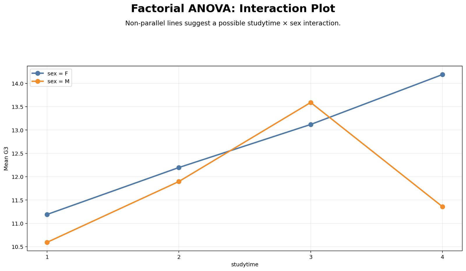
This interaction plot compares female and male mean G3 across studytime groups. The female line rises steadily from group 1 through group 4. The male line rises from group 1 to group 3, then drops sharply at group 4.
The two lines are not parallel, which visually suggests that the relationship between studytime and G3 may differ by sex. The strongest visual difference appears at studytime group 4, where the female mean is high while the male mean is much lower.
The p-value chart must be used with this visual pattern. The interaction plot shows a possible interaction shape, but the formal interaction p value is about 0.08323, which is above the .05 threshold. The correct conclusion is visible non-parallel lines without a statistically significant interaction at alpha = .05.
Python Chart 2: Cell Means
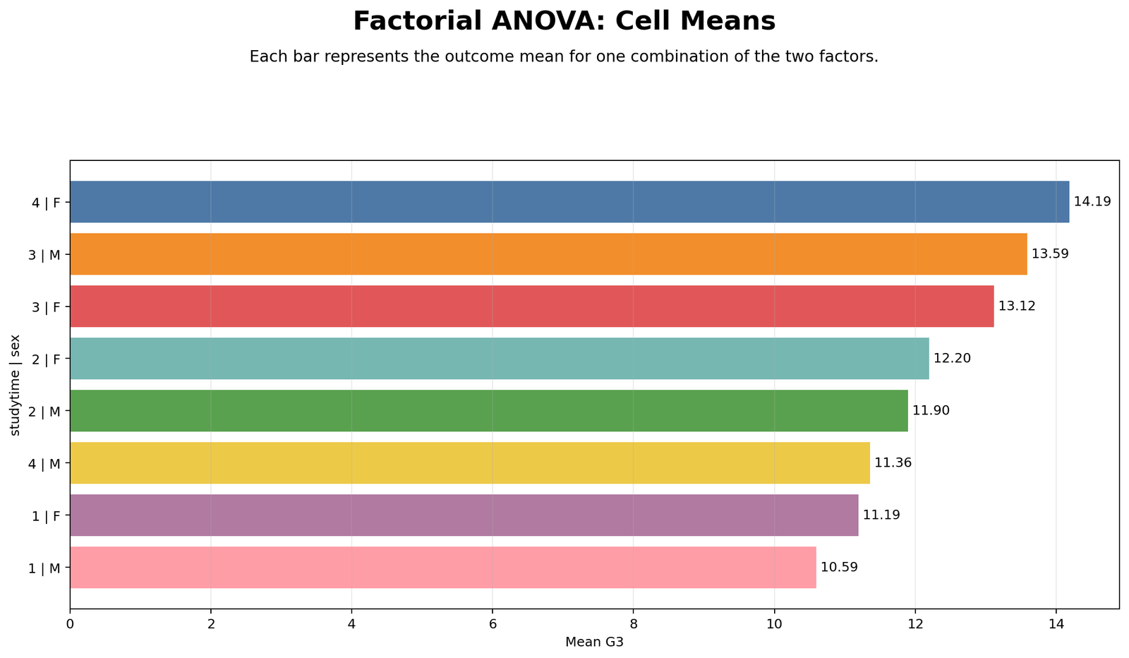
This chart ranks the mean G3 values for each combination of studytime and sex. The lowest cell mean is 1 | M = 10.59, followed by 1 | F = 11.19. The highest cell mean is 4 | F = 14.19, followed by 3 | M = 13.59 and 3 | F = 13.12.
The cell means show why the interaction plot is not perfectly parallel. Female students continue upward into studytime group 4, while male students peak in studytime group 3 and then drop in group 4.
This chart gives the best practical explanation of the model. Factorial ANOVA is not only about marginal means; it also studies the individual combinations of the factors.
Python Chart 3: Main Effect of Studytime
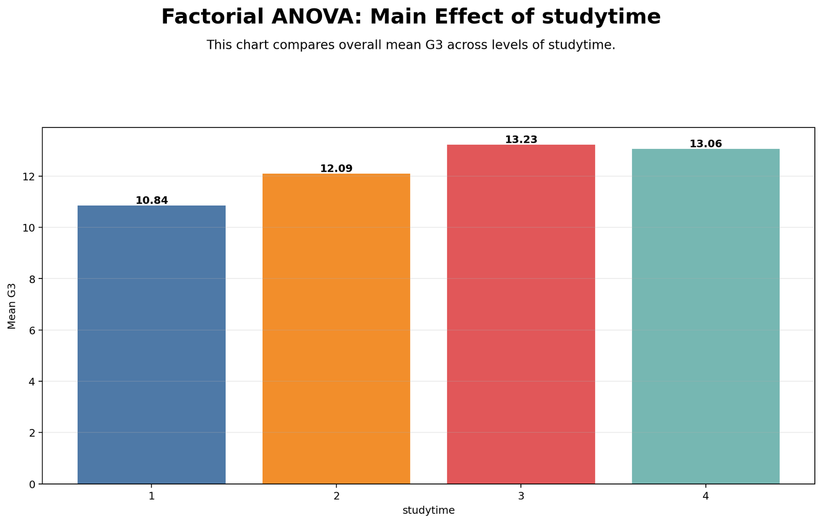
This chart shows the overall mean G3 for each studytime level after averaging across sex. The means increase from group 1 to group 3 and remain high in group 4. The visible values are about 10.84 for group 1, 12.09 for group 2 and about 13.23 for group 3, with group 4 near the same high range.
The studytime pattern is the strongest result in the factorial ANOVA. The p-value summary places the studytime effect far below the alpha line, so studytime is statistically significant.
This chart should be used to explain the main finding. Higher studytime levels are associated with higher G3 means, even after the model includes sex and the interaction term.
Python Chart 4: Main Effect of Sex
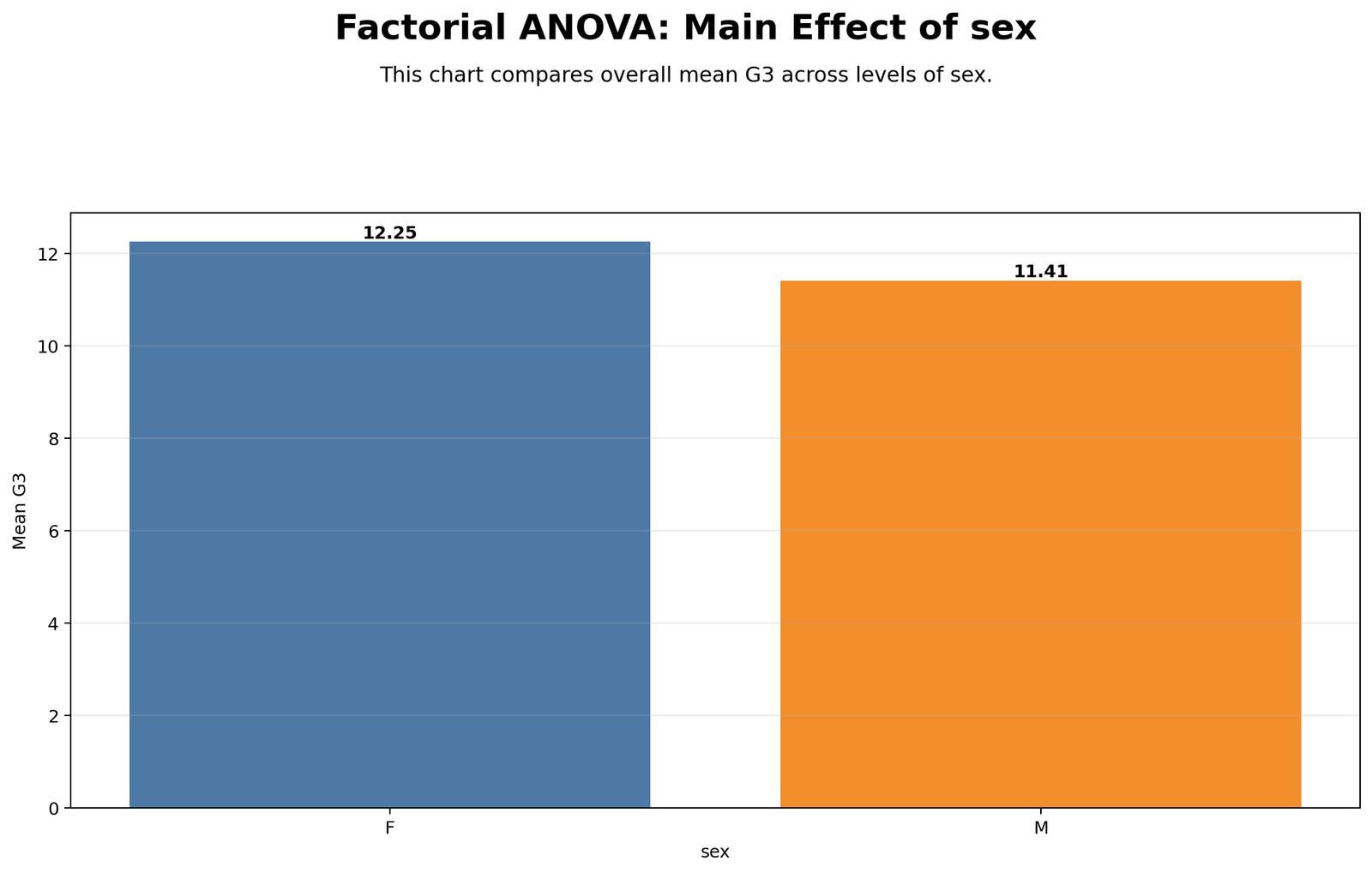
This chart compares overall mean G3 between female and male students. The female mean is about 12.25, while the male mean is about 11.41. The chart therefore shows a higher average G3 for female students.
The p-value summary shows that this difference does not reach the .05 threshold. The sex p value is about 0.07362, which is above .05.
The correct interpretation is that the sample shows a visible female-male mean difference, but the factorial ANOVA does not declare the sex main effect statistically significant at the 5% level.
Python Chart 5: P-Value Decision Summary
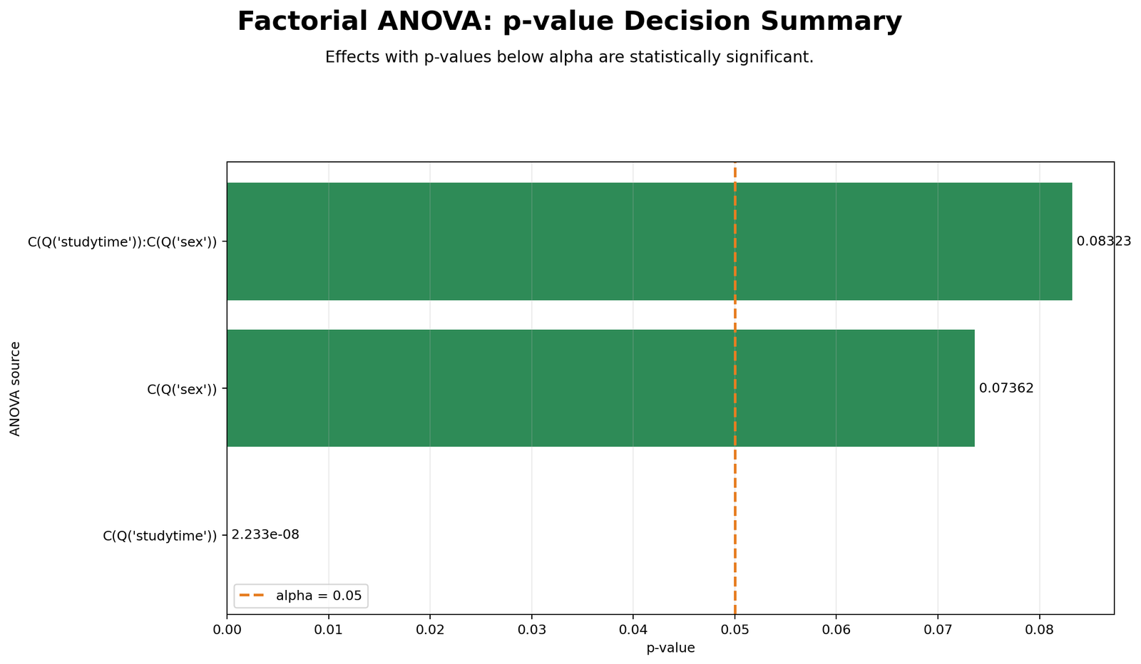
This chart compares the p values for the factorial ANOVA sources with the alpha line at 0.05. The studytime p value is extremely small and is placed far to the left of the alpha line. The sex p value is about 0.07362, and the interaction p value is about 0.08323.
The chart gives the formal decision. Studytime is statistically significant because its p value is below .05. Sex and the studytime × sex interaction are not statistically significant because their p values are above .05.
This chart is the most important statistical decision summary. It prevents over-reading the interaction plot by showing that the visible non-parallel pattern is not significant at alpha .05.
Python Chart 6: Effect Size Summary
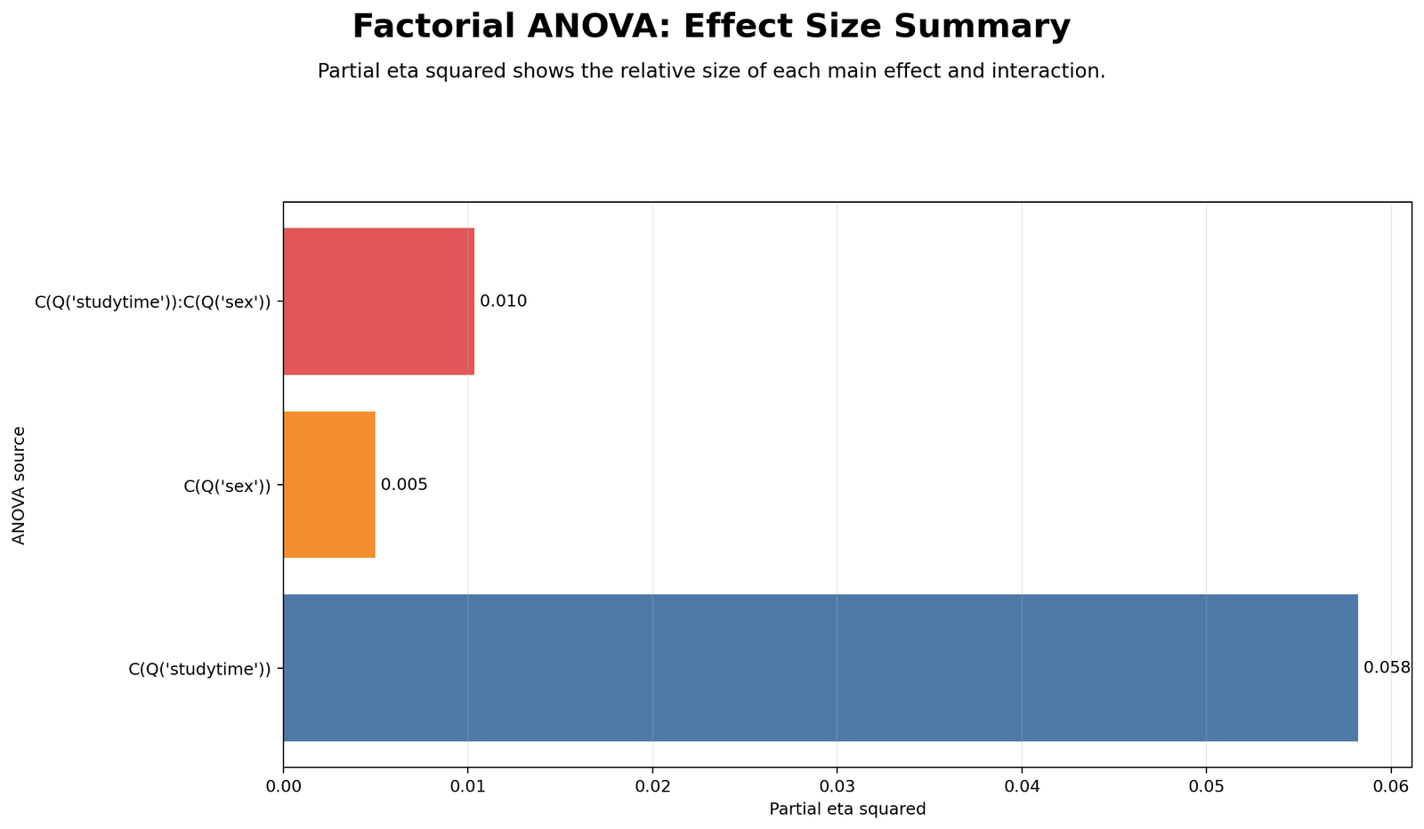
This chart summarizes the practical size of the factorial ANOVA effects with partial eta squared. The bars are shown on a wide partial eta squared scale, so the effects appear very small visually.
The effect-size chart should be read with the p-value chart. Studytime is statistically significant, while sex and the interaction do not cross the .05 threshold. The practical-size summary does not support a large-effect claim for any source.
The safest reporting approach is to state the significance decisions first, then report effect sizes as supporting information. In this example, the studytime effect is the meaningful source to discuss, while sex and the interaction are not significant at alpha .05.
Python Chart 7: Residuals vs Fitted Values
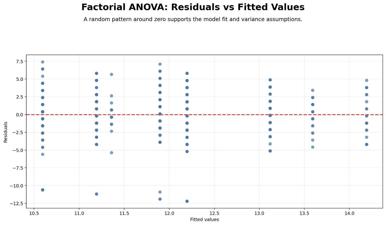
This residual plot shows residuals against fitted values from the factorial ANOVA model. The points appear in vertical groups because each fitted value corresponds to a studytime-sex cell mean. Most residuals are centered around the zero line.
Several large negative residuals appear below the main cloud, especially around fitted values near 11.2, 11.9 and 12.2. These cases represent students whose observed G3 scores were much lower than their fitted cell mean.
The diagnostic conclusion is that the model captures the group structure, but some low-score cases create a negative residual tail. These cases should be mentioned in the assumptions section rather than ignored.
Python Chart 8: Residual Q-Q Plot
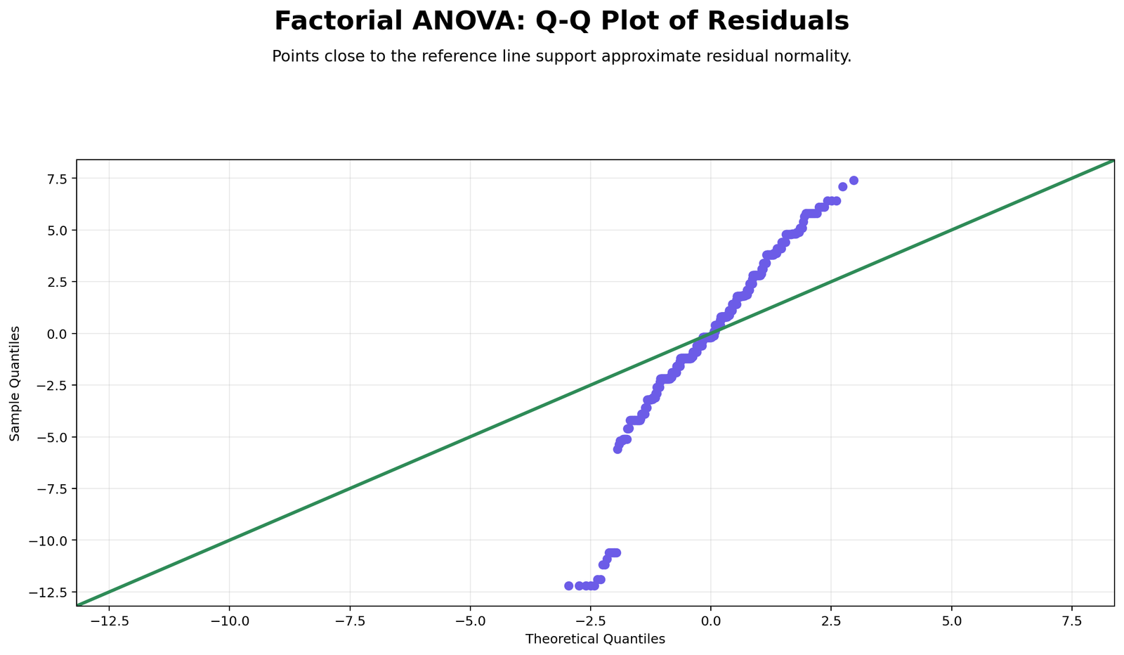
The Q-Q plot compares the residual distribution with a normal reference line. The middle part of the residual distribution is closer to the reference line, but the lower tail moves far below the line.
The largest departures occur on the negative side, matching the residuals-versus-fitted chart. This shows that a small group of students scored far below the model’s fitted cell mean.
The Q-Q plot does not change the main studytime result, but it adds diagnostic context. The final report should state that the main effect of studytime is significant while residual diagnostics show lower-tail departures from normality.
R Chart-by-Chart Validation
The R validation charts repeat the same factorial ANOVA workflow in a second software environment. They confirm the interaction shape, cell means, main effects, p-value decisions, effect-size context and residual diagnostic pattern.
R Chart 1: Interaction Plot
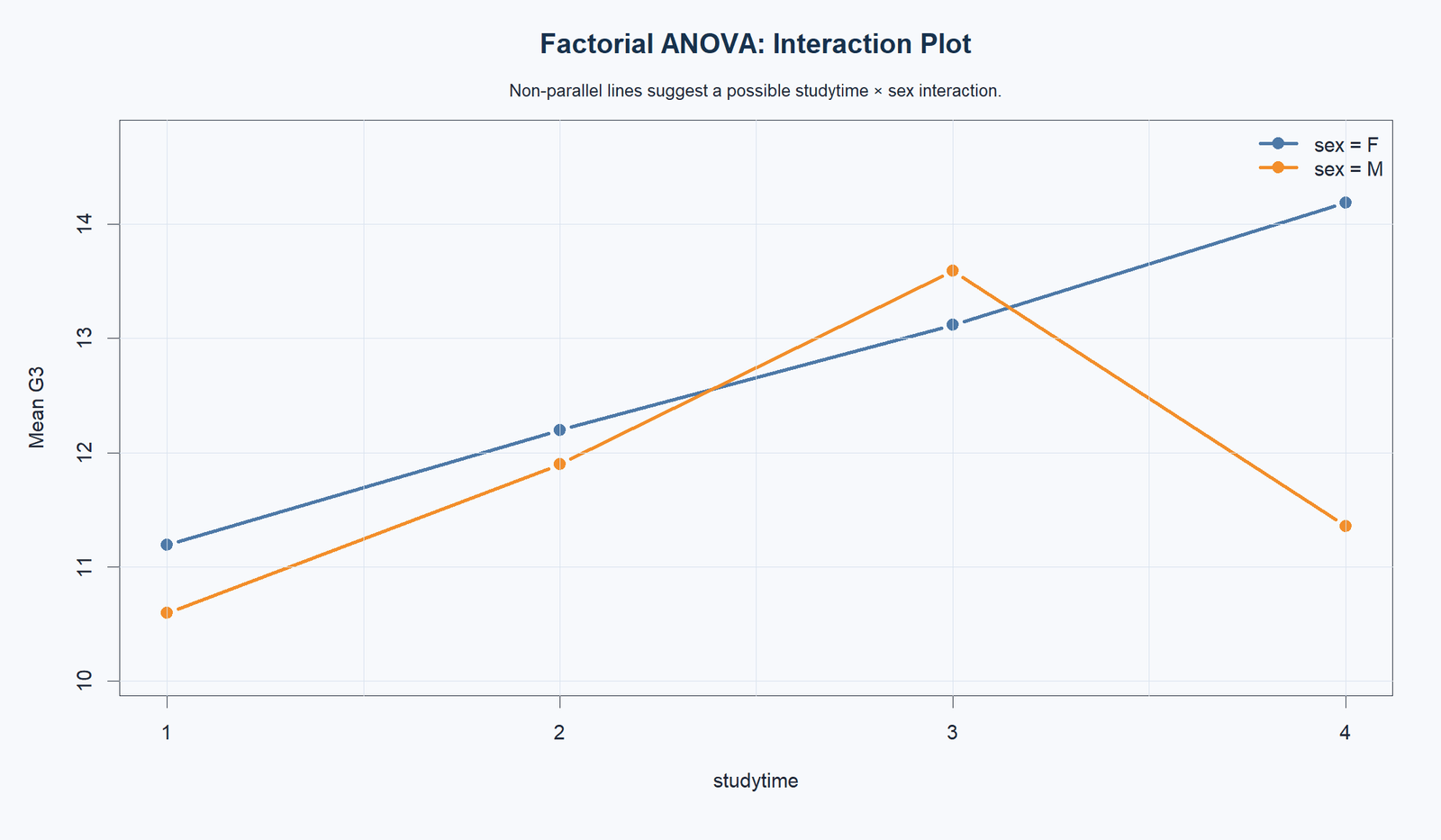
This R chart confirms the non-parallel pattern between female and male students. The female line increases steadily across studytime groups, while the male line rises through group 3 and then falls in group 4.
The visible shape is important, but it must still be interpreted with the interaction p value. The supplied p-value chart reports the interaction above .05, so the visual interaction is not statistically significant at alpha .05.
This chart validates the Python interaction plot and supports the same conclusion: discuss the visible pattern, but do not claim a statistically significant interaction.
R Chart 2: Cell Means
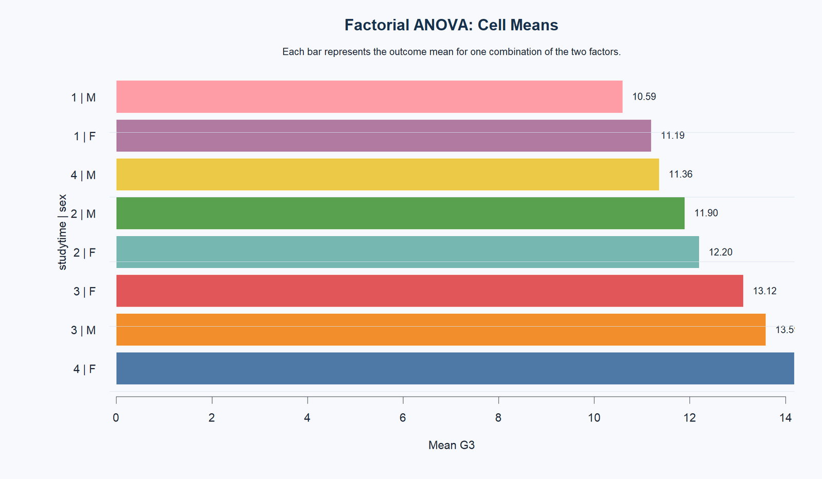
This R chart confirms the cell mean ranking. The lowest mean appears for 1 | M = 10.59, while the highest mean appears for 4 | F = 14.19. The values for studytime group 3 are high for both sexes, with male students around 13.59 and female students around 13.12.
The chart makes the interaction pattern easier to understand. The female group reaches its highest value at studytime group 4, while the male group peaks at group 3 and then falls at group 4.
In reporting, this chart should be used after the interaction plot because it shows the exact cell combinations responsible for the plotted line pattern.
R Chart 3: Main Effect of Studytime
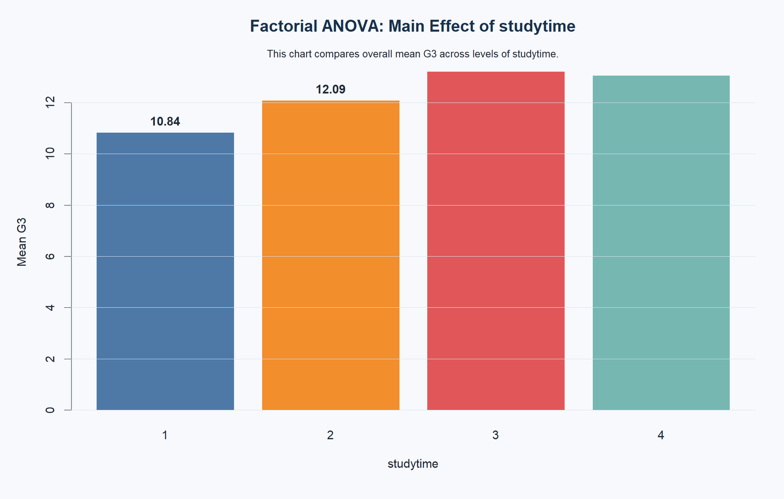
This R chart confirms the main effect of studytime. The mean G3 is about 10.84 at studytime group 1 and about 12.09 at group 2, then rises into the higher range for groups 3 and 4.
This pattern matches the p-value decision chart, where studytime is the significant source. The visible increase in means explains why the studytime main effect is the central result of the factorial ANOVA.
The final interpretation should emphasize studytime first. It is the factor that clearly crosses the statistical decision threshold in the supplied chart set.
R Chart 4: Main Effect of Sex
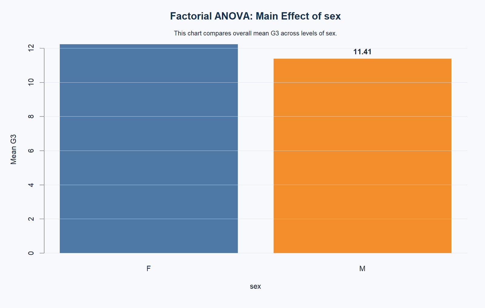
This R chart confirms that the female mean G3 is higher than the male mean G3. The female mean is about 12.25, and the male mean is about 11.41.
The p-value decision chart shows that this difference is not statistically significant at the .05 level because the sex p value is about 0.07362. The visible difference is therefore reported as a sample pattern, not as a statistically significant main effect.
This chart supports careful wording. Do not write that sex significantly affects G3 at .05; write that female students had a higher sample mean, but the main effect of sex did not reach the .05 significance level.
R Chart 5: P-Value Decision Summary
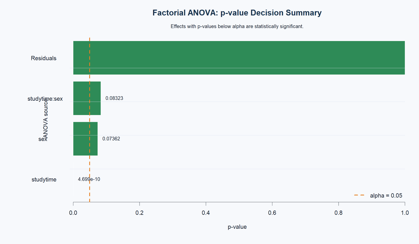
This R chart confirms the same decision pattern. Studytime is below the alpha threshold, while sex is about 0.07362 and the studytime × sex interaction is about 0.08323.
The chart includes the .05 alpha line, making the decision direct. Only effects to the left of that line are statistically significant at the 5% level.
The R validation result agrees with the Python workflow: studytime is significant, sex is not significant at .05, and the interaction is not significant at .05.
R Chart 6: Effect Size Summary
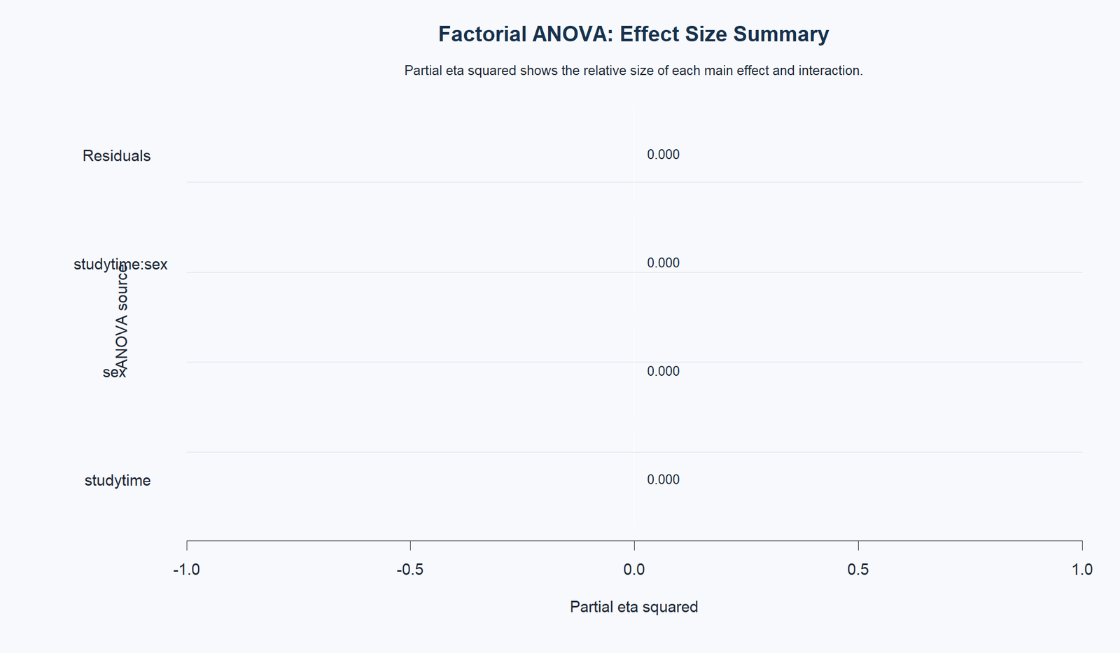
This R chart displays the partial eta squared context for the factorial ANOVA sources. The bars are visually tiny on the chart scale, so the effect sizes should not be presented as large.
The effect-size chart should be interpreted alongside the p-value chart. Studytime is the statistically supported effect, while sex and the interaction do not reach significance at alpha .05.
In final reporting, effect sizes should be used as supporting context. The strongest practical message remains the significant studytime effect and the non-significant sex and interaction tests.
R Chart 7: Residuals vs Fitted Values
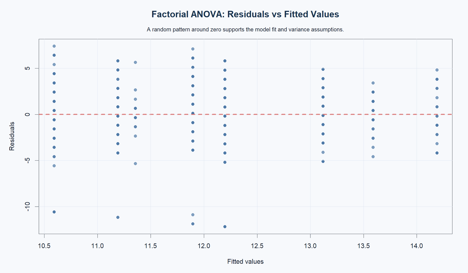
The R residuals-versus-fitted chart confirms the same vertical-band pattern as the Python chart. The fitted values represent studytime-sex cell means, and most residuals are centered around zero.
Several negative residuals fall well below the main pattern. These cases represent students whose observed G3 scores were much lower than the fitted value for their cell.
The chart supports a balanced diagnostic statement. The factorial ANOVA model is useful for the studytime effect, but the residual diagnostics show lower-tail cases that should be mentioned.
R Chart 8: Residual Q-Q Plot
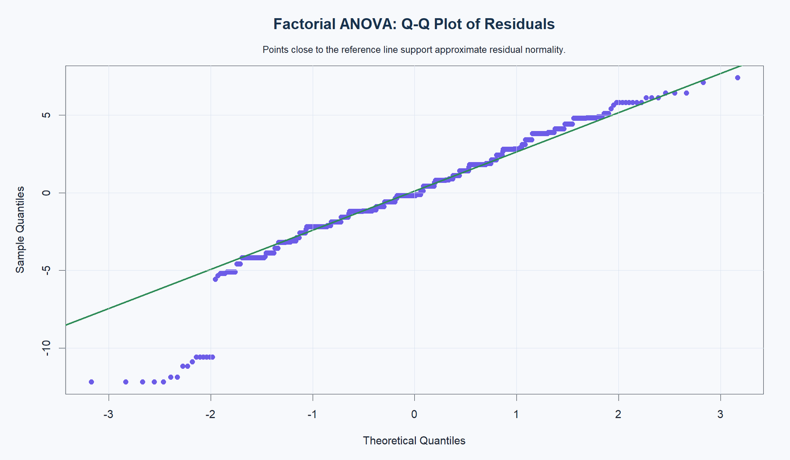
The R Q-Q plot confirms that the central residuals are closer to the reference line, while the lower tail departs from the line. This matches the Python Q-Q plot.
The lower-tail departure means some observations are much lower than the model expects from their studytime-sex cell. This should be reported as a diagnostic limitation or assumption note.
The Q-Q plot does not remove the significant studytime effect. It adds context: the model finds a clear studytime difference, while residual normality is not perfect because of low-tail cases.
SPSS Output and Report PDFs
The supplied report files provide downloadable support for the Factorial ANOVA workflow. The Python report, R report and SPSS output PDF should be linked in the resources section and used as verification files for the WordPress article.
Download Factorial ANOVA Python Report PDF
Download Factorial ANOVA R Report PDF
Download Factorial ANOVA SPSS Output PDF
Output Items to Read
| Output Item | What It Shows | How It Is Used | Reporting Meaning |
|---|---|---|---|
| Interaction plot | Studytime pattern by sex. | Checks whether lines are parallel. | Visible non-parallel pattern, but interaction p is above .05. |
| Cell means | Mean G3 for each studytime-sex combination. | Explains the interaction pattern. | Highest cell is 4 | F, lowest cell is 1 | M. |
| Main effect of studytime | Overall mean G3 by studytime. | Tests studytime after averaging across sex. | Significant effect. |
| Main effect of sex | Overall mean G3 by sex. | Tests sex after averaging across studytime. | Not significant at .05. |
| P-value summary | Studytime, sex and interaction p values. | Gives formal decisions. | Only studytime is significant at .05. |
| Residual diagnostics | Residuals vs fitted and Q-Q plot. | Checks model assumptions. | Lower-tail departures should be reported. |
Report interpretation summary: The Factorial ANOVA report supports a significant studytime main effect on G3. The sex main effect and studytime × sex interaction are not significant at alpha .05 in the supplied p-value summaries. The residual diagnostics show lower-tail cases, so the final report should include an assumptions note.
SPSS, R, Python and Excel Workflows for Factorial ANOVA
The same Factorial ANOVA workflow can be reproduced in SPSS, R, Python and Excel. The key steps are to define the two categorical factors, fit a model with main effects and interaction, read the ANOVA table, inspect interaction and cell means, report effect sizes and check residual diagnostics.
SPSS Workflow
| Step | SPSS Menu or Syntax | Purpose |
|---|---|---|
| Open data | File > Open > Data | Load G3, studytime and sex. |
| Run model | Analyze > General Linear Model > Univariate | Fit factorial ANOVA. |
| Set dependent variable | Dependent Variable: G3 | Define the numeric outcome. |
| Set fixed factors | Fixed Factors: studytime and sex | Define categorical factors. |
| Request interaction | Model: Full factorial | Test studytime, sex and studytime × sex. |
| Request plots | Plots: studytime on horizontal axis, sex as separate lines | Create interaction plot. |
| Request effect size | Options > Estimates of effect size | Display partial eta squared. |
| Export output | OUTPUT EXPORT | Save SPSS output PDF. |
R Workflow
| Step | R Action | Purpose |
|---|---|---|
| Read data | read.csv("dataset.csv") | Load the dataset. |
| Convert factors | as.factor(studytime) and as.factor(sex) | Ensure categorical treatment. |
| Fit model | aov(G3 ~ studytime * sex) | Run factorial ANOVA. |
| Read ANOVA table | summary(model) | Get main effects and interaction p values. |
| Cell means | aggregate(G3 ~ studytime + sex) | Explain interaction pattern. |
| Diagnostics | plot(model) | Check residuals and Q-Q plot. |
Python Workflow
| Step | Python Action | Purpose |
|---|---|---|
| Read data | pandas.read_csv() | Load dataset. |
| Fit model | ols("G3 ~ C(studytime) * C(sex)") | Fit factorial ANOVA. |
| ANOVA table | sm.stats.anova_lm(model, typ=2) | Read main effects and interaction. |
| Cell means | groupby(["studytime","sex"]) | Calculate cell means. |
| Effect size | Partial eta squared formula | Compare source sizes. |
| Diagnostics | Residual plots and Q-Q plot | Check model assumptions. |
Excel Workflow
| Excel Task | Formula or Tool | Purpose |
|---|---|---|
| Arrange data | Rows for studytime and columns for sex | Create two-factor layout. |
| Run ANOVA | Data Analysis ToolPak > ANOVA: Two-Factor With Replication | Run factorial ANOVA when cells have repeated observations. |
| Read rows effect | Rows source | Usually one factor such as studytime. |
| Read columns effect | Columns source | Usually second factor such as sex. |
| Read interaction | Interaction source | Test whether factor effects depend on each other. |
| Decision | Compare p values with alpha | Reject H0 when p < .05. |
Code Blocks for Factorial ANOVA
SPSS Syntax for Factorial ANOVA
* Factorial ANOVA / Two-Way ANOVA in SPSS.
* Dependent variable: G3.
* Fixed factors: studytime and sex.

TITLE "Factorial ANOVA: G3 by Studytime and Sex".

UNIANOVA G3 BY studytime sex
  /METHOD=SSTYPE(3)
  /INTERCEPT=INCLUDE
  /PLOT=PROFILE(studytime*sex)
  /PRINT=DESCRIPTIVE ETASQ HOMOGENEITY
  /EMMEANS=TABLES(studytime)
  /EMMEANS=TABLES(sex)
  /EMMEANS=TABLES(studytime*sex)
  /CRITERIA=ALPHA(.05)
  /DESIGN=studytime sex studytime*sex.

OUTPUT EXPORT
  /CONTENTS EXPORT=VISIBLE
  /PDF DOCUMENTFILE="factorial_anova_output.pdf".
Python Code for Factorial ANOVA
import pandas as pd
import numpy as np
import statsmodels.api as sm
from statsmodels.formula.api import ols

df = pd.read_csv("dataset.csv")

df["G3"] = pd.to_numeric(df["G3"], errors="coerce")
df["studytime"] = df["studytime"].astype("category")
df["sex"] = df["sex"].astype("category")

df_model = df.dropna(subset=["G3", "studytime", "sex"]).copy()

# Factorial ANOVA model with main effects and interaction
model = ols("G3 ~ C(studytime) * C(sex)", data=df_model).fit()

anova_table = sm.stats.anova_lm(model, typ=2)
print(anova_table)

# Cell means
cell_means = (
    df_model
    .groupby(["studytime", "sex"])["G3"]
    .agg(["count", "mean", "std"])
    .reset_index()
)
print(cell_means)

# Main effects
studytime_means = df_model.groupby("studytime")["G3"].mean()
sex_means = df_model.groupby("sex")["G3"].mean()

print("Studytime means")
print(studytime_means)

print("Sex means")
print(sex_means)

# Partial eta squared
ss_error = anova_table.loc["Residual", "sum_sq"]

effect_sizes = {}
for source in anova_table.index:
    if source != "Residual":
        ss_effect = anova_table.loc[source, "sum_sq"]
        effect_sizes[source] = ss_effect / (ss_effect + ss_error)

print("Partial eta squared")
print(effect_sizes)

# Residual diagnostics
df_model["fitted"] = model.fittedvalues
df_model["residual"] = model.resid

print(df_model[["G3", "studytime", "sex", "fitted", "residual"]].head())
R Code for Factorial ANOVA
df <- read.csv("dataset.csv")

df$G3 <- as.numeric(df$G3)
df$studytime <- as.factor(df$studytime)
df$sex <- as.factor(df$sex)

df_model <- na.omit(df[, c("G3", "studytime", "sex")])

# Factorial ANOVA model
model <- aov(G3 ~ studytime * sex, data = df_model)

summary(model)

# Cell means
aggregate(G3 ~ studytime + sex, data = df_model, FUN = function(x) {
  c(n = length(x), mean = mean(x), sd = sd(x))
})

# Main effect means
aggregate(G3 ~ studytime, data = df_model, mean)
aggregate(G3 ~ sex, data = df_model, mean)

# Diagnostic values
df_model$fitted <- fitted(model)
df_model$residuals <- residuals(model)

# Residual diagnostics
plot(model)

# Optional interaction plot
interaction.plot(
  x.factor = df_model$studytime,
  trace.factor = df_model$sex,
  response = df_model$G3,
  fun = mean,
  xlab = "studytime",
  ylab = "Mean G3",
  trace.label = "sex"
)
Excel Formulas and Tool Steps for Factorial ANOVA
Excel Tool:
Data > Data Analysis > ANOVA: Two-Factor With Replication

Use this when:
- Factor 1 = studytime
- Factor 2 = sex
- Outcome = G3
- Each studytime-sex cell has repeated observations

Decision rule:
If p-value for rows < alpha, factor 1 is significant.
If p-value for columns < alpha, factor 2 is significant.
If p-value for interaction < alpha, interaction is significant.

Alpha:
0.05

Example interpretation from this output:
studytime = significant
sex = not significant at .05
studytime × sex = not significant at .05

Cell mean:
=AVERAGE(cell_range)

Cell standard deviation:
=STDEV.S(cell_range)

Decision formula:
=IF(p_value<0.05,"Reject H0","Fail to reject H0")
APA Reporting Wording
When reporting Factorial ANOVA, report the main effects and interaction separately. Do not only report the strongest effect. The reader needs to know whether each factor and their interaction were significant.
APA-style report: A factorial ANOVA was used to examine the effects of studytime and sex on G3 final grade. The main effect of studytime was statistically significant, indicating that mean G3 differed across studytime levels. The main effect of sex was not statistically significant at alpha = .05, p ≈ .07362. The studytime × sex interaction was also not statistically significant at alpha = .05, p ≈ .08323. Cell means showed that female students in studytime group 4 had the highest mean G3, while male students in studytime group 1 had the lowest mean G3.
Short reporting version: The factorial ANOVA showed a significant main effect of studytime on G3, while the sex main effect and the studytime × sex interaction were not significant at the .05 level.
Common Mistakes
| Mistake | Why It Is Wrong | Correct Practice |
|---|---|---|
| Ignoring the interaction | Factorial ANOVA is designed to test whether factors work together. | Always report main effects and interaction. |
| Calling a visible interaction significant | Non-parallel lines can appear even when p > .05. | Use the p-value decision with the plot. |
| Reporting only studytime | The model also tests sex and studytime × sex. | Report all ANOVA sources. |
| Confusing cell means with main effects | Cell means are factor combinations; main effects are marginal means. | Interpret both separately. |
| Ignoring residual diagnostics | ANOVA depends on reasonable residual and variance behavior. | Check residuals vs fitted, Q-Q plot, Levene Test and Brown-Forsythe Test. |
| Skipping effect size | Significance does not show practical size. | Add ANOVA Effect Size, Effect Size or Cohen’s F Formula. |
When to Use Factorial ANOVA
Use Factorial ANOVA when the dependent variable is numeric and the research question includes two or more categorical factors. It is especially useful when the analyst wants to test both main effects and interactions in the same model.
| Situation | Use Factorial ANOVA? | Reporting Note |
|---|---|---|
| One numeric outcome and two categorical factors | Yes | Report both main effects and interaction. |
| Testing whether factor effects depend on each other | Yes | Use interaction term. |
| Only one categorical factor | No | Use one-way ANOVA. |
| One numeric covariate included | Use ANCOVA | See the ANCOVA guide. |
| Repeated-measures factor included | Use repeated-measures ANOVA | Check sphericity and corrections. |
For related guides, see ANOVA in Python, ANOVA in R, ANOVA in SPSS, ANOVA Assumptions, ANOVA Effect Size, Balanced ANOVA, Brown Forsythe ANOVA, ANCOVA, and T Test vs ANOVA.
Downloads and Resources for Factorial ANOVA
Use these resources to reproduce the Factorial ANOVA workflow. The Python report, R report and SPSS output PDF are included as verification files. Script and workbook placeholders can be replaced after the final files are uploaded to the WordPress Media Library.
Download Dataset
Practice dataset with G3, studytime and sex variables.
Download Factorial ANOVA Python Report PDF
Python report PDF for interaction plot, cell means, main effects and diagnostics.
Download Factorial ANOVA R Report PDF
R validation PDF for factorial ANOVA results and chart confirmation.
Download Factorial ANOVA SPSS Output PDF
SPSS output PDF for factorial ANOVA interpretation and reporting.
Download Python Script
Python code for two-way ANOVA, cell means, effect size and residual diagnostics.
Download R Script and Excel Workbook
R workflow and Excel two-factor ANOVA template.
FAQs About Factorial ANOVA
What is Factorial ANOVA?
Factorial ANOVA is an ANOVA model that tests two or more categorical factors and their interaction effects on one numeric outcome.
What is the difference between one-way ANOVA and Factorial ANOVA?
One-way ANOVA tests one categorical factor. Factorial ANOVA tests two or more factors and can test interactions between them.
What was the main result in this example?
The main effect of studytime was significant. The main effect of sex and the studytime × sex interaction were not significant at alpha .05.
Was the interaction significant?
No. The interaction p value was about 0.08323, which is above .05. The plot shows non-parallel lines, but the formal interaction test was not significant at the 5% level.
What was the sex main-effect result?
The female mean G3 was higher than the male mean G3 in the sample, but the sex p value was about 0.07362, so the effect was not significant at alpha .05.
What cell had the highest mean G3?
The highest cell mean was studytime group 4 for female students, with mean G3 about 14.19.
What cell had the lowest mean G3?
The lowest cell mean was studytime group 1 for male students, with mean G3 about 10.59.
Can Factorial ANOVA be done in Excel?
Yes. Excel Data Analysis ToolPak has ANOVA: Two-Factor With Replication, which can be used when the data are arranged in a two-factor layout with repeated observations.
What should be checked before reporting Factorial ANOVA?
Check group means, interaction plot, p-value summary, effect size, residuals versus fitted values, Q-Q plot and equal-variance assumption checks.
How do I report this Factorial ANOVA in APA style?
A concise report is: A factorial ANOVA showed a significant main effect of studytime on G3, while the sex main effect and studytime × sex interaction were not significant at the .05 level.

