
Regression Diagnostics, Residual Variance and Heteroskedasticity
White Test is a regression diagnostic test used to check whether model residuals have constant variance. In simple words, it tests the homoscedasticity assumption. This guide explains the White Test for heteroskedasticity with null hypothesis, alternative hypothesis, formula, SPSS output, Python charts, R validation charts and Excel workflow using a regression model where G3 final grade is predicted from G1, G2, studytime, failures, absences and age.
Quick Answer: White Test Result
The White Test result indicates that the regression residuals do not have constant variance. The base regression predicting G3 from G1, G2, studytime, failures, absences and age explained a large share of variation in final grades, with base model R² = 0.8506 in the Python/R summary and R² = .851 in the SPSS output. However, the White auxiliary regression, which models squared residuals using predictors, squared terms and interaction terms, produced auxiliary R² = 0.1164. The White LM p-value was 1.753e-06, which is far below α = .05.
Hypothesis decision: The null hypothesis for the White Test says that residual variance is constant, or H0: homoscedasticity. The alternative hypothesis says that residual variance is not constant, or H1: heteroskedasticity. Since p = 1.753e-06 < .05, reject the null hypothesis. The final conclusion is that there is statistically significant evidence of heteroskedasticity in the G3 regression residuals.
Final report sentence: A White Test for heteroskedasticity was performed on the residuals from the regression predicting G3 final grade from G1, G2, studytime, failures, absences and age. The auxiliary regression explained a meaningful share of squared residual variation, R² = 0.1164, producing a significant White LM test, p = 1.753e-06. Therefore, the null hypothesis of constant residual variance was rejected. The model shows evidence of heteroskedasticity, so robust standard errors or a corrected modeling strategy should be considered.
Important note: Do not write p = .000 in the final report. SPSS displays very small p-values as .000, but the correct reporting style is p < .001. The Python p-value chart gives the more precise value 1.753e-06, which also means p < .001.
Table of Contents
- What Is the White Test?
- When Should You Use the White Test?
- Null and Alternative Hypothesis for White Test
- White Test Formula and LM Statistic
- Dataset and Regression Model Used
- Verified SPSS, Python and R Results
- Python Charts and Interpretation
- R Validation Charts and Interpretation
- SPSS Output Interpretation
- How to Run White Test in Python, R, SPSS and Excel
- How to Report the White Test
- Common Mistakes
- Downloads and Resources
- FAQs
What Is the White Test?
The White Test is a statistical test for detecting heteroskedasticity in regression residuals. Heteroskedasticity means that the variance of the residuals is not constant across fitted values or predictor levels. A well-behaved ordinary least squares regression model usually assumes that residuals have approximately constant variance. When this assumption fails, coefficient estimates may still be unbiased under standard OLS conditions, but the usual standard errors, t-tests, confidence intervals and p-values can become unreliable.
The White Test is more general than many simple heteroskedasticity tests because it does not only check a straight-line relationship between residual variance and predictors. It uses an auxiliary regression where squared residuals are regressed on the original predictors, squared predictors and cross-product interaction terms. This allows the test to detect many different variance patterns, including curved variance patterns and interaction-based variance patterns.
For regression diagnostics, the White Test should be read together with residual plots and related assumption checks. If your main concern is variance equality across groups, you may also compare it with Levene Test and Brown-Forsythe Test. If your concern is changing variance across ordered fitted values or time-like order, the Goldfeld-Quandt Test can also be useful. For normality context, residual plots can be compared with Q-Q Plot, P-P Plot, Kolmogorov-Smirnov Test, Lilliefors Test and DAgostino Pearson Test.
Practical meaning: If the White Test is significant, it means the residual spread is related to the predictors, squared predictors or interactions. In this post, the p-value is extremely small, so the G3 regression model should not be reported with ordinary OLS standard errors alone. A better reporting approach is to mention heteroskedasticity and consider robust standard errors.
When Should You Use the White Test?
Use the White Test when you fit a regression model and want to test whether the residual variance is constant. It is especially useful when you suspect that residual spread may change in a nonlinear way or may depend on combinations of predictors. Because the White Test includes squares and interaction terms in its auxiliary regression, it can detect more complex heteroskedasticity patterns than a very simple residual variance test.
| Situation | Use White Test? | Why it helps |
|---|---|---|
| Linear regression with continuous predictors | Yes | It checks whether residual variance changes with fitted values, predictors, squared predictors or interactions. |
| Residuals vs fitted plot shows a funnel shape | Yes | The White Test provides a formal p-value for the visual pattern. |
| You need an assumption test before reporting OLS results | Yes | It supports a clear decision about constant variance. |
| You only want to compare group variances | Maybe | Levene or Brown-Forsythe may be easier if the problem is purely group-based. |
| You only want to test residual normality | No | White Test is a heteroskedasticity test, not a normality test. Use Q-Q plots and normality tests for residual shape. |
Null and Alternative Hypothesis for White Test
The White Test is a hypothesis test. The decision is based on whether the auxiliary regression explains enough variation in squared residuals to reject the idea of constant residual variance.
| Hypothesis | Statement | Meaning in this G3 model |
|---|---|---|
| Null hypothesis | H0: residual variance is constant | The regression errors for G3 have homoscedastic variance across fitted values and predictors. |
| Alternative hypothesis | H1: residual variance is not constant | The residual variance changes with predictors, squared predictors or interactions. |
| Decision rule | Reject H0 if p < α | Using α = .05, the result is significant because p = 1.753e-06. |
Decision for this post: The White LM p-value is 1.753e-06. Since this is below .05 and also below .001, reject the null hypothesis. The result supports the alternative hypothesis that the residual variance is not constant.
White Test Formula and LM Statistic
The White Test is usually calculated from an auxiliary regression. The steps are simple in concept:
| Step | What is done? | Purpose |
|---|---|---|
| 1 | Fit the main OLS regression. | Get fitted values and residuals from the model. |
| 2 | Square the residuals. | Squared residuals represent local variance size. |
| 3 | Regress squared residuals on predictors, squared predictors and interactions. | This is the White auxiliary regression. |
| 4 | Take the auxiliary R². | A larger auxiliary R² means residual variance is more predictable. |
| 5 | Calculate LM = n × R². | The LM statistic is compared with a chi-square distribution. |
White LM statistic = n × R²(auxiliary regression)

where:
n = sample size
R²(auxiliary regression) = R-squared from the regression of squared residuals on auxiliary terms
For this analysis, n = 649 and the auxiliary model summary chart gives R² = 0.1164. Therefore, the LM statistic is approximately:
LM ≈ 649 × 0.1164
LM ≈ 75.54
The auxiliary regression included 27 auxiliary terms in the full model. The p-value from the chi-square decision is 1.753e-06. This very small p-value means the squared residuals are not random noise around a constant variance level. Instead, their size is related to the predictor structure.
Dataset and Regression Model Used
This worked example uses the student performance data structure. The dependent variable is G3 final grade. The base regression predicts G3 from G1, G2, studytime, failures, absences and age. The White Test is then applied to the residuals from that base regression.
| Item | Value | Explanation |
|---|---|---|
| Dependent variable | G3 | Final grade / main outcome variable. |
| Base predictors | G1, G2, studytime, failures, absences, age | Variables used to predict G3 before residual diagnostics. |
| Valid N | 649 | All 649 cases were used in the regression and residual diagnostics. |
| SPSS-ready file | White-Test-data.sav | Clean SPSS file used for the output PDF. |
| Output type | Python charts, R charts, SPSS PDF and Excel method | Python and R validate the graphics and test decision; SPSS provides formal regression output. |
External dataset source: UCI Machine Learning Repository: Student Performance dataset.
Verified SPSS, Python and R Results
The SPSS output, Python charts and R charts all support the same decision: the White Test is statistically significant. The base model has strong predictive fit, but the residual variance is not constant. The auxiliary regression explains enough squared residual variation to reject homoscedasticity.
Base Regression Output
| Statistic | SPSS value | Python/R chart value | Interpretation |
|---|---|---|---|
| Model R | .922 | Approximately .922 | The predicted G3 values are strongly associated with observed G3 values. |
| R Square | .851 | 0.8506 | The base model explains about 85% of G3 variation. |
| Adjusted R Square | .849 | Approximately .849 | The model remains strong after adjusting for predictors. |
| Std. Error of Estimate | 1.254 | Approximately 1.254 | Typical prediction error is about 1.25 grade points. |
| ANOVA F | F(6, 642) = 609.353, p < .001 | Significant | The base regression model is statistically significant. |
Base Regression Coefficients
| Predictor | B | t | p-value | Interpretation |
|---|---|---|---|---|
| G1 | .142 | 3.886 | p < .001 | G1 is a significant positive predictor of G3 after controlling for the other variables. |
| G2 | .883 | 25.823 | p < .001 | G2 is the strongest predictor in the base model. |
| studytime | .095 | 1.526 | .127 | Study time is not significant after G1 and G2 are included. |
| failures | -.233 | -2.456 | .014 | More failures are associated with lower G3, controlling for the other predictors. |
| absences | .023 | 2.086 | .037 | Absences have a small positive coefficient in this controlled model. |
| age | .024 | .544 | .587 | Age is not a significant predictor in the base model. |
White Auxiliary Regression Output
| Auxiliary model | Auxiliary terms included | R² | F-test | Meaning |
|---|---|---|---|---|
| Block 1 | Original predictors and squared predictors | .070 | F = 3.986, p < .001 | Even the first auxiliary block detects variance structure. |
| Block 2 | Block 1 plus several grade and predictor interactions | .102 | F = 3.380, p < .001 | Interactions improve the explanation of squared residuals. |
| Block 3 | Full White-style auxiliary model with 27 terms | .116 / 0.1164 | F = 3.030, p < .001 | This is the final auxiliary model used for the White decision. |
Final White Test Decision
| Component | Result | Decision |
|---|---|---|
| Null hypothesis | H0: residual variance is constant | Assumes homoscedasticity. |
| Alternative hypothesis | H1: residual variance is not constant | Assumes heteroskedasticity. |
| Auxiliary R² | 0.1164 | Squared residuals are partly explained by auxiliary terms. |
| White LM p-value | 1.753e-06 | Reject H0. |
| Alpha level | .05 | The p-value is far below the decision threshold. |
| Conclusion | Significant heteroskedasticity | Use robust standard errors or revise the model strategy. |
Python Charts and Interpretation
1. White Test: Residuals vs Fitted Values
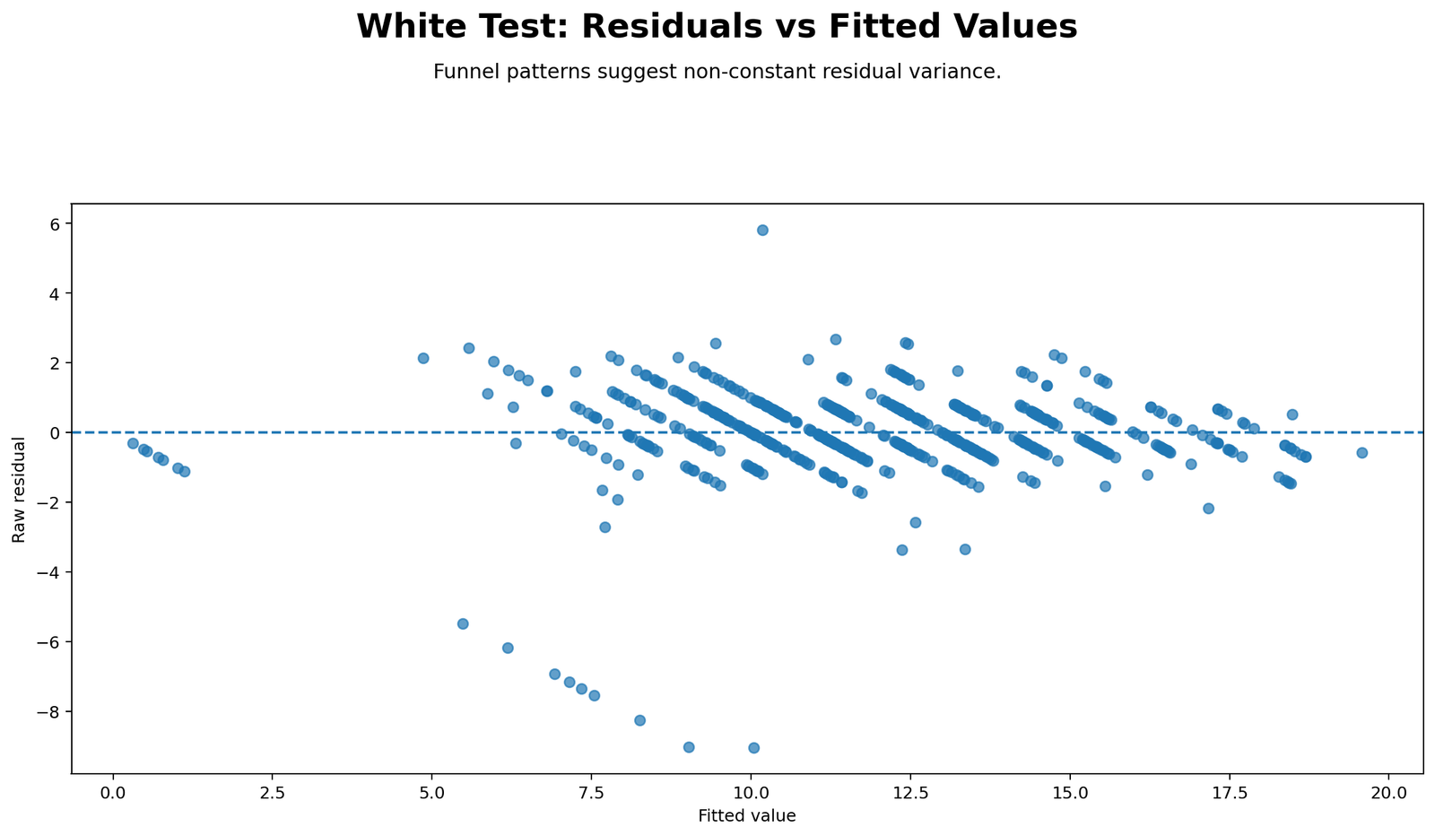
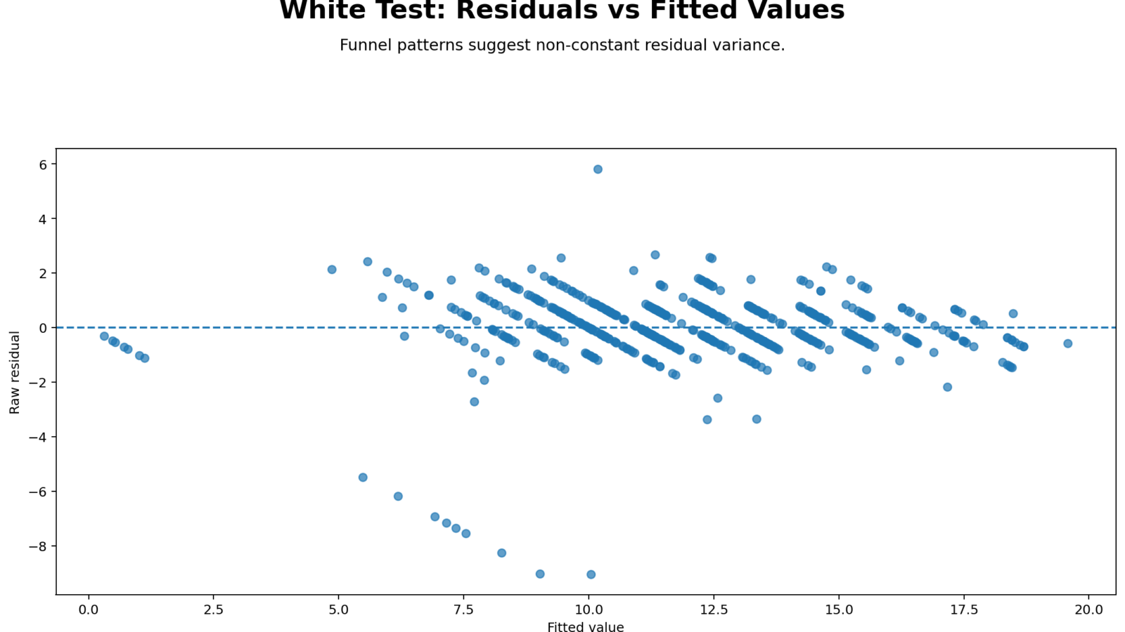
This chart is the first visual diagnostic for the White Test. If residual variance were constant, the points would form a fairly even horizontal band around zero across the fitted-value range. Instead, the chart shows an uneven residual spread. Some fitted-value regions have tight residual bands, while the middle fitted range contains large negative residuals and wider vertical spread. Several residuals drop below -6 and even approach about -9, while positive residuals are smaller in comparison. This visual pattern supports the White Test result because residual variance is not evenly distributed across fitted values. The dashed zero line confirms that the residuals are centered around zero overall, but the problem is the changing spread, not the average residual.
2. White Test: Squared Residuals vs Fitted Values
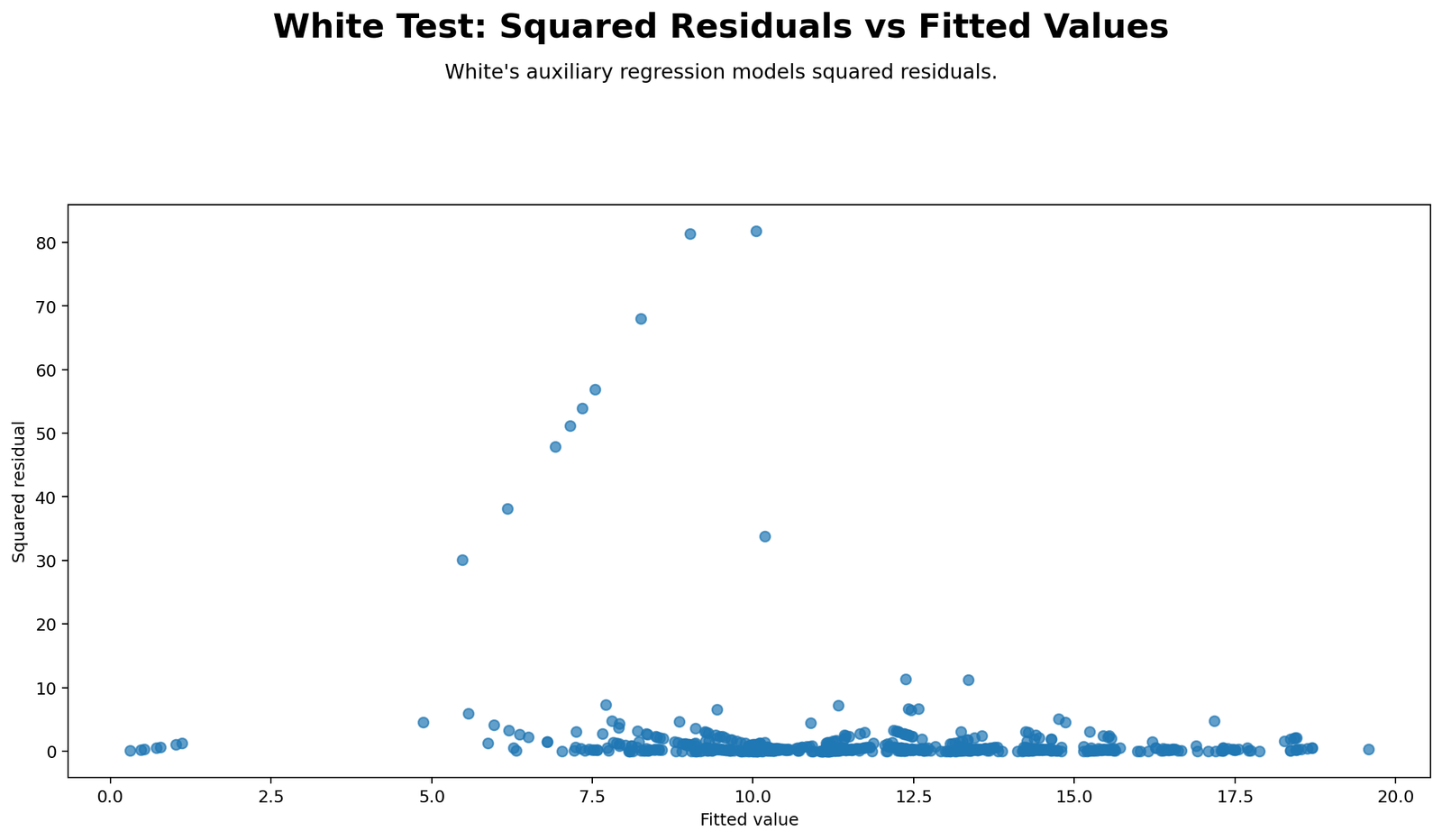
This chart directly connects to the White auxiliary regression because the auxiliary regression uses squared residuals as the dependent variable. Most squared residuals are close to zero, but several observations rise sharply, with the largest squared residuals above 80. These large values are concentrated mainly in the mid fitted-value range rather than being evenly distributed across all fitted values. That is exactly the type of pattern that can make the White Test significant. The chart shows that the residual variance is not simply random and flat; instead, some fitted-value regions produce much larger error sizes than others.
3. White Test: Absolute Residual Spread
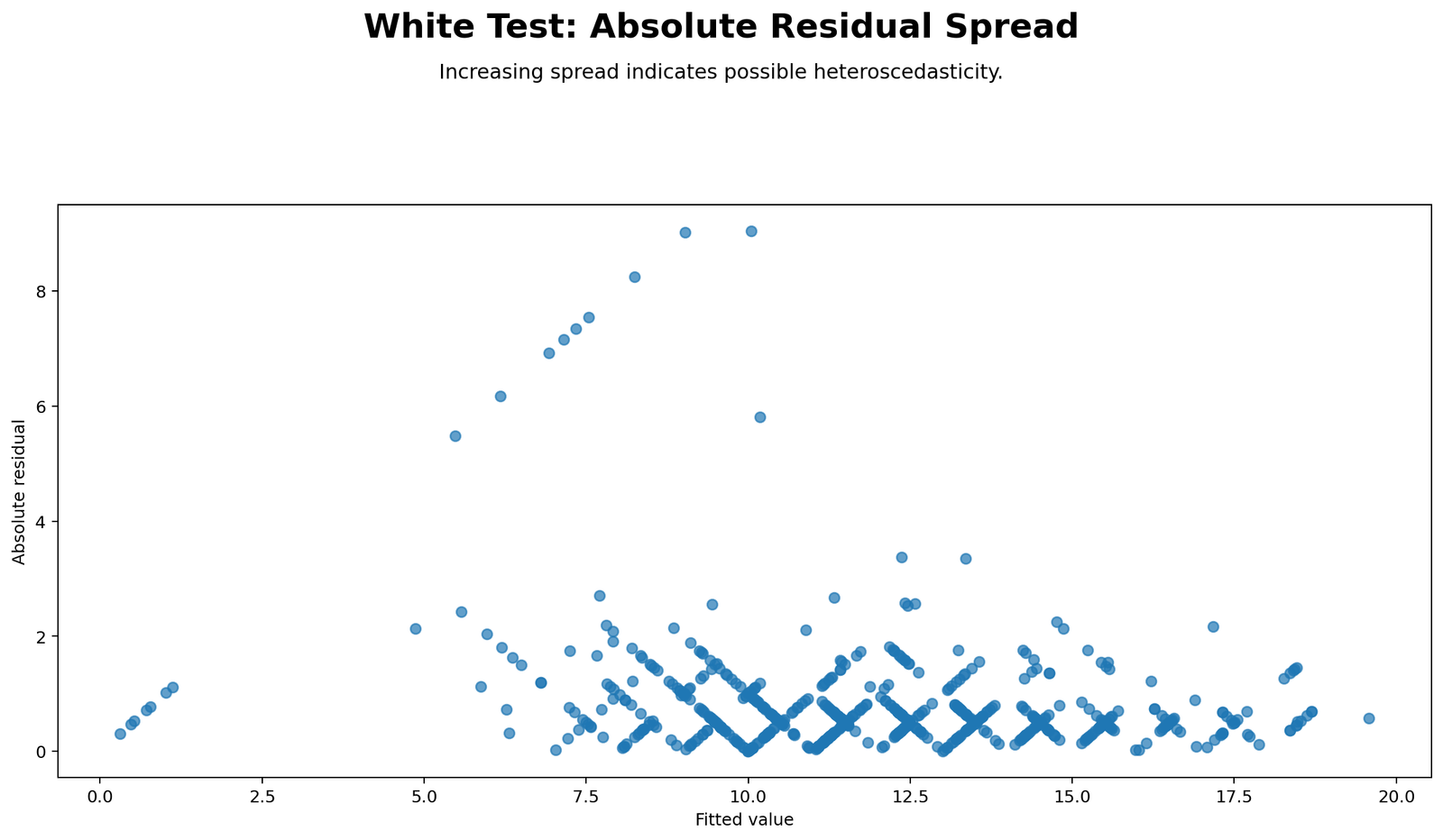
The absolute residual chart removes the positive or negative sign and focuses only on error size. This makes spread easier to read. A constant-variance model would show a roughly similar range of absolute residuals across fitted values. Here, the largest absolute residuals appear around the middle fitted-value range, reaching around 9. Other fitted-value regions have much smaller absolute residuals. This uneven spread supports the decision to reject the null hypothesis of homoscedasticity. It also explains why a model can have a high base R² but still fail the constant variance assumption: prediction accuracy and residual variance stability are different diagnostics.
4. White Test: p-value Decision
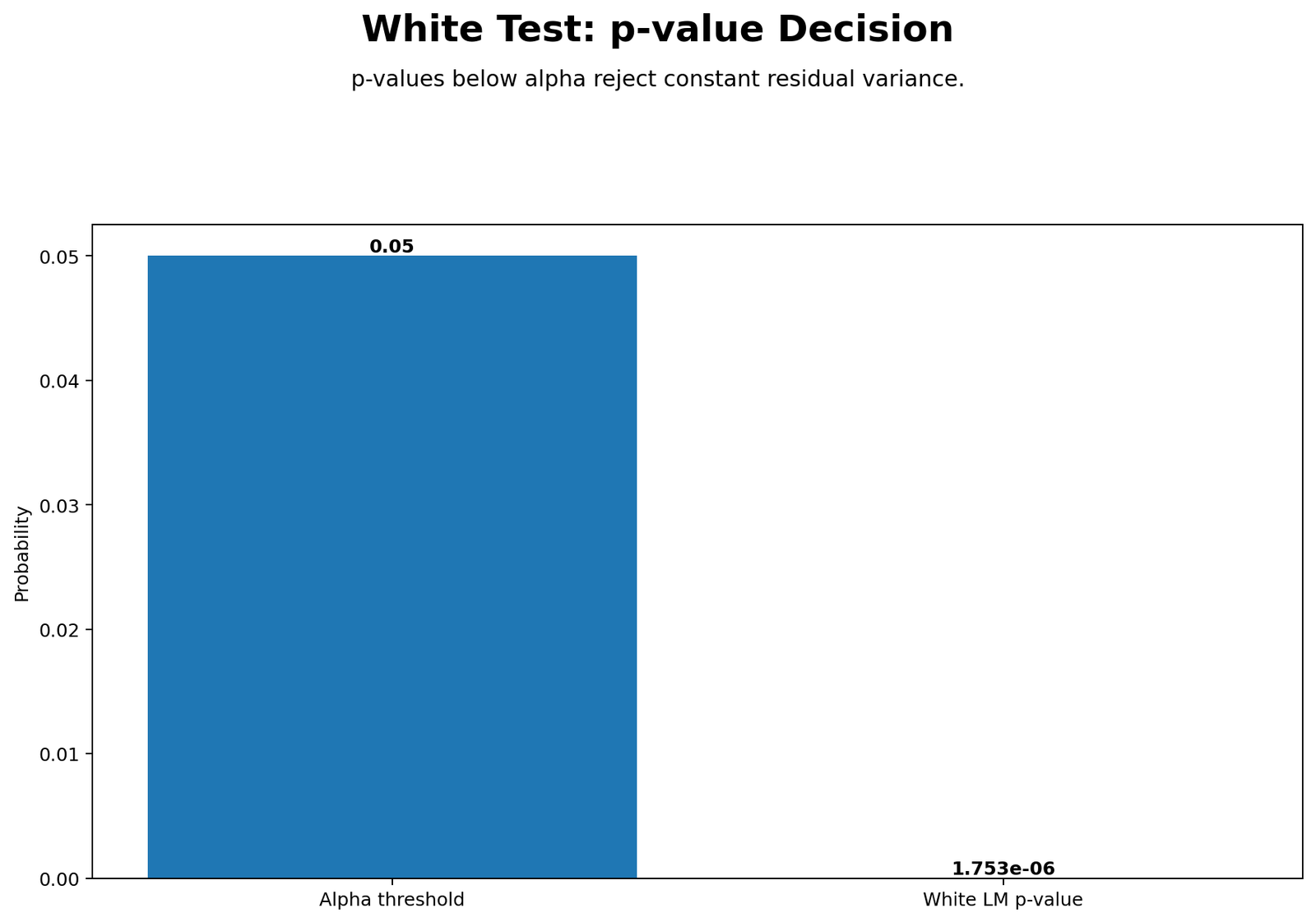
This chart gives the formal hypothesis decision. The alpha threshold is .05, while the White LM p-value is 1.753e-06. Because the p-value is much smaller than .05, the test rejects the null hypothesis. In reporting language, this means there is statistically significant evidence of heteroskedasticity. The chart is useful for readers because it makes the decision rule visible: p-values below alpha reject constant residual variance.
5. White Test: Strongest Auxiliary Terms
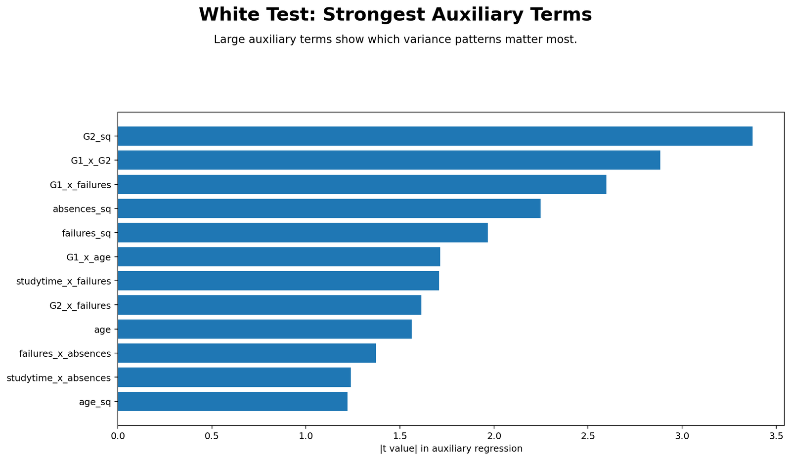
This chart shows which auxiliary terms contributed most strongly to explaining squared residuals. The largest terms are G2_sq, G1_x_G2, G1_x_failures, absences_sq and failures_sq. These terms suggest that the residual variance pattern is connected to grade-related nonlinear effects and interactions involving previous grades and failures. In practical terms, the error spread is not constant across the grade structure. Some combinations of prior grades, failures and absences create larger prediction errors than others. This supports the White Test decision because the squared residuals are meaningfully associated with auxiliary terms.
6. White Test: Residual Distribution
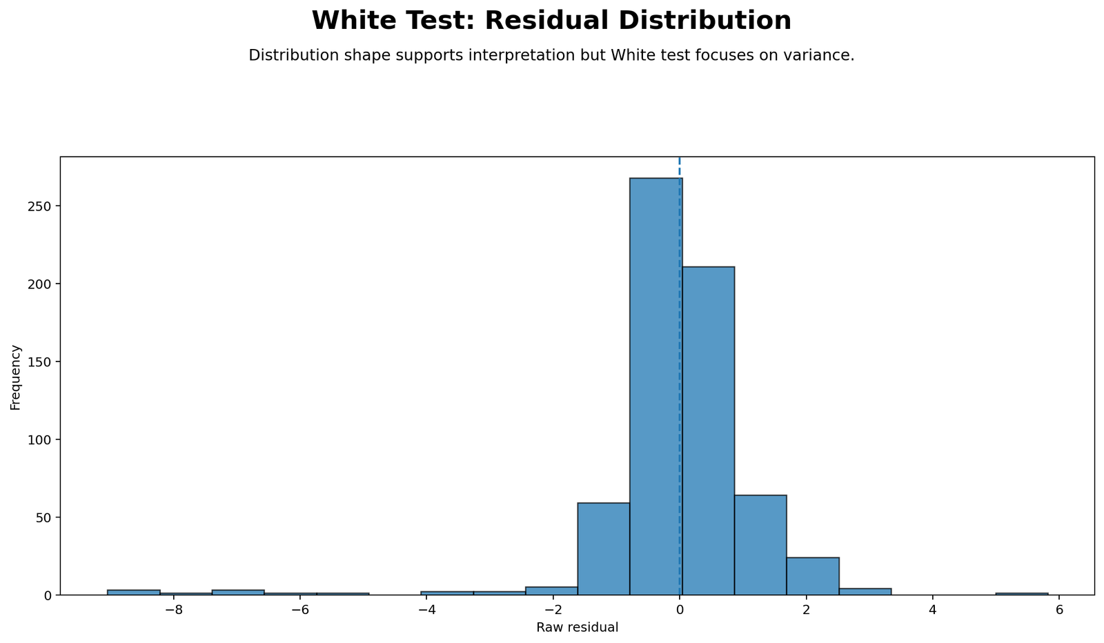
The residual distribution is centered near zero, which is expected in an OLS regression with an intercept. However, the distribution is not perfectly symmetric. The left tail is longer because several residuals are strongly negative. This chart does not replace the White Test because residual normality and residual variance are different assumptions. Still, it helps explain why the residual plots show large negative errors and why squared residuals have extreme values. The main White Test decision remains based on the variance pattern and p-value, not only on histogram shape.
7. White Test: Base and Auxiliary Model Fit
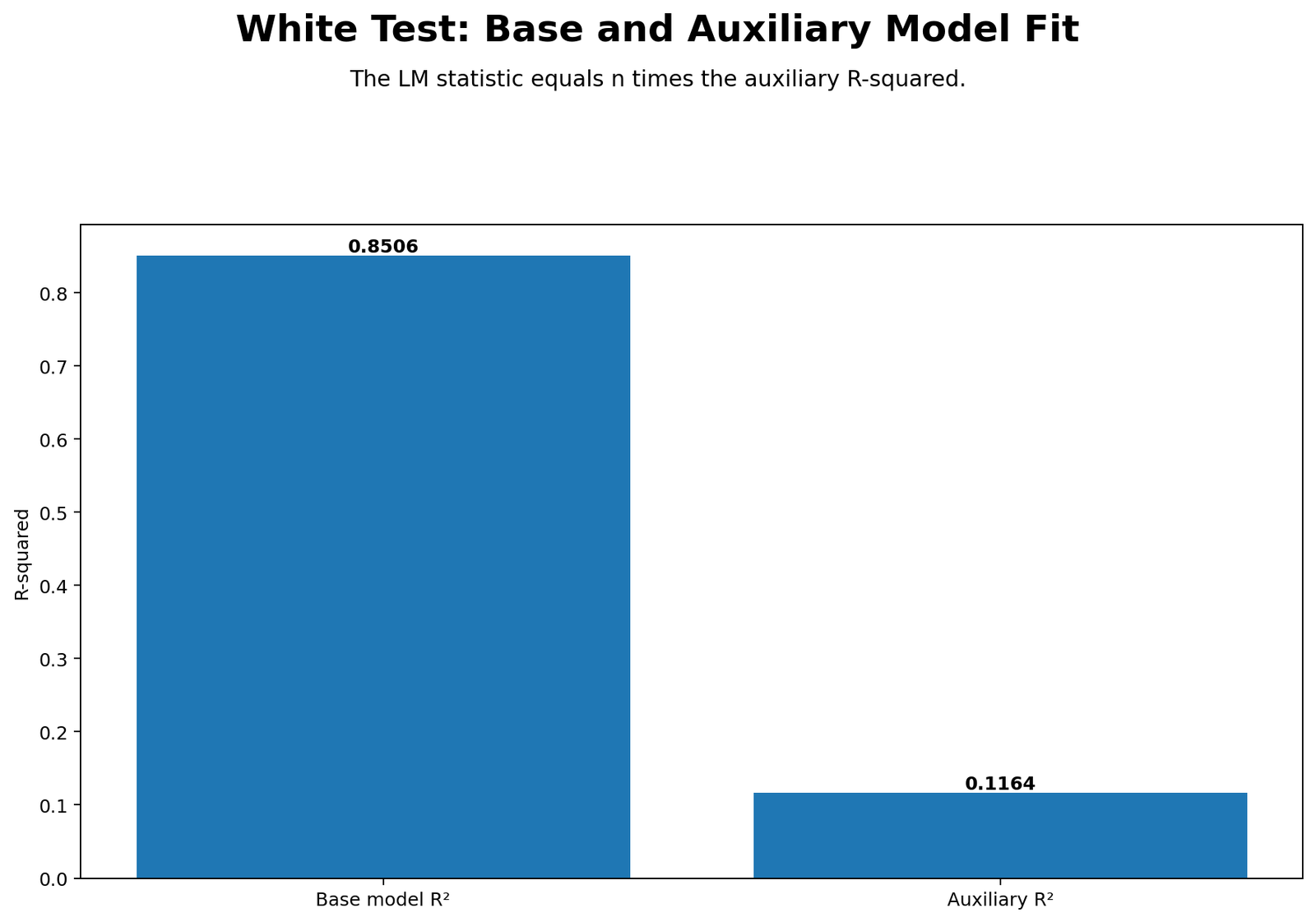
This chart separates two different ideas. The base model R² of 0.8506 means the predictors explain G3 very well. The auxiliary R² of 0.1164 means the auxiliary terms explain part of the squared residual variation. A high base model R² does not protect the model from heteroskedasticity. The auxiliary R² is smaller than the base R², but for a White Test it is large enough to produce a significant LM p-value because the sample size is 649. The chart therefore supports the final conclusion: the model predicts G3 well, but the residual variance assumption is violated.
R Validation Charts and Interpretation
The R charts validate the same diagnostic story shown by Python. They use a different plotting style but show the same fitted-value range, residual spread, squared residual behavior, p-value decision, auxiliary term importance, residual distribution and model-fit comparison.
1. R Residuals vs Fitted Values
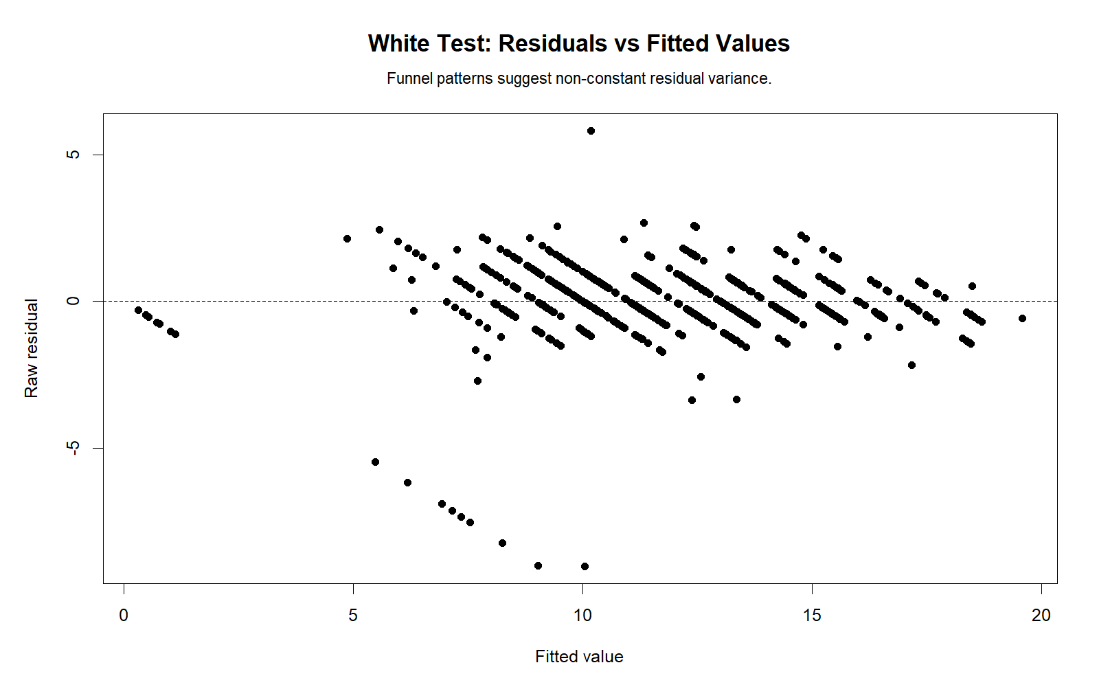
The R residuals-vs-fitted chart confirms that the residual spread is not uniform. Several large negative residuals appear in the middle fitted-value region, while many other fitted ranges have smaller error bands. This validates the Python interpretation that the residual variance is not constant across the fitted-value scale.
2. R Squared Residuals vs Fitted Values
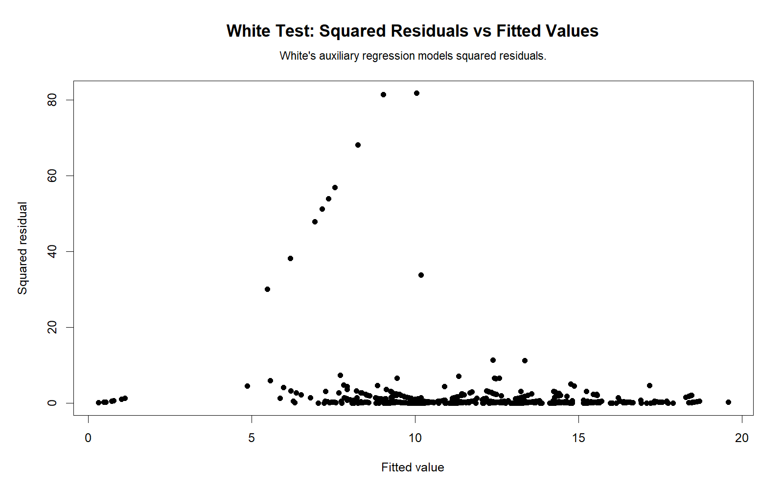
The R squared-residual plot again shows that most squared residuals are small, but a few are very large. These high squared residuals create the variance pattern detected by the auxiliary regression. The chart is especially important because White’s auxiliary regression directly models squared residuals.
3. R Absolute Residual Spread
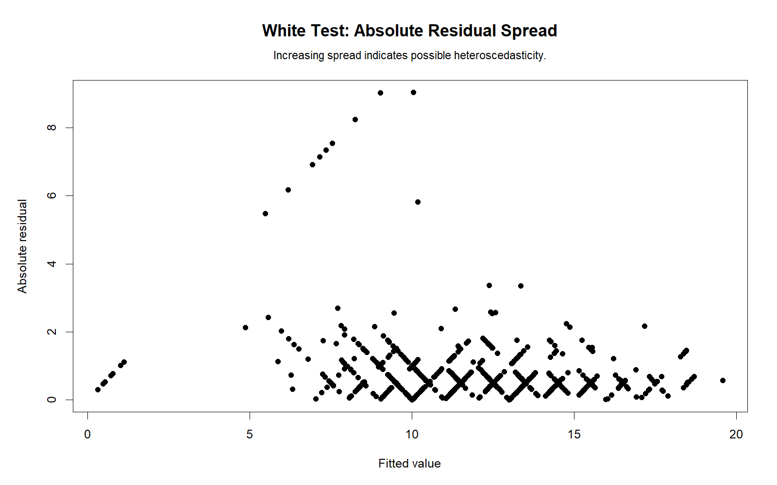
The R absolute residual chart confirms the uneven error size. The largest absolute residuals appear around the middle fitted range. This means the model error is not equally spread across all predictions, which supports the rejection of homoscedasticity.
4. R p-value Decision
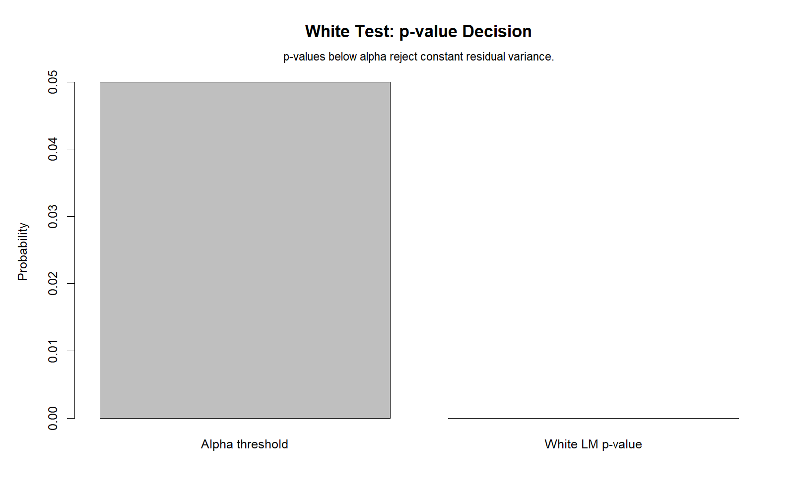
The R p-value chart repeats the same hypothesis decision: the White LM p-value is below the alpha threshold. Therefore, the null hypothesis of constant residual variance is rejected.
5. R Strongest Auxiliary Terms
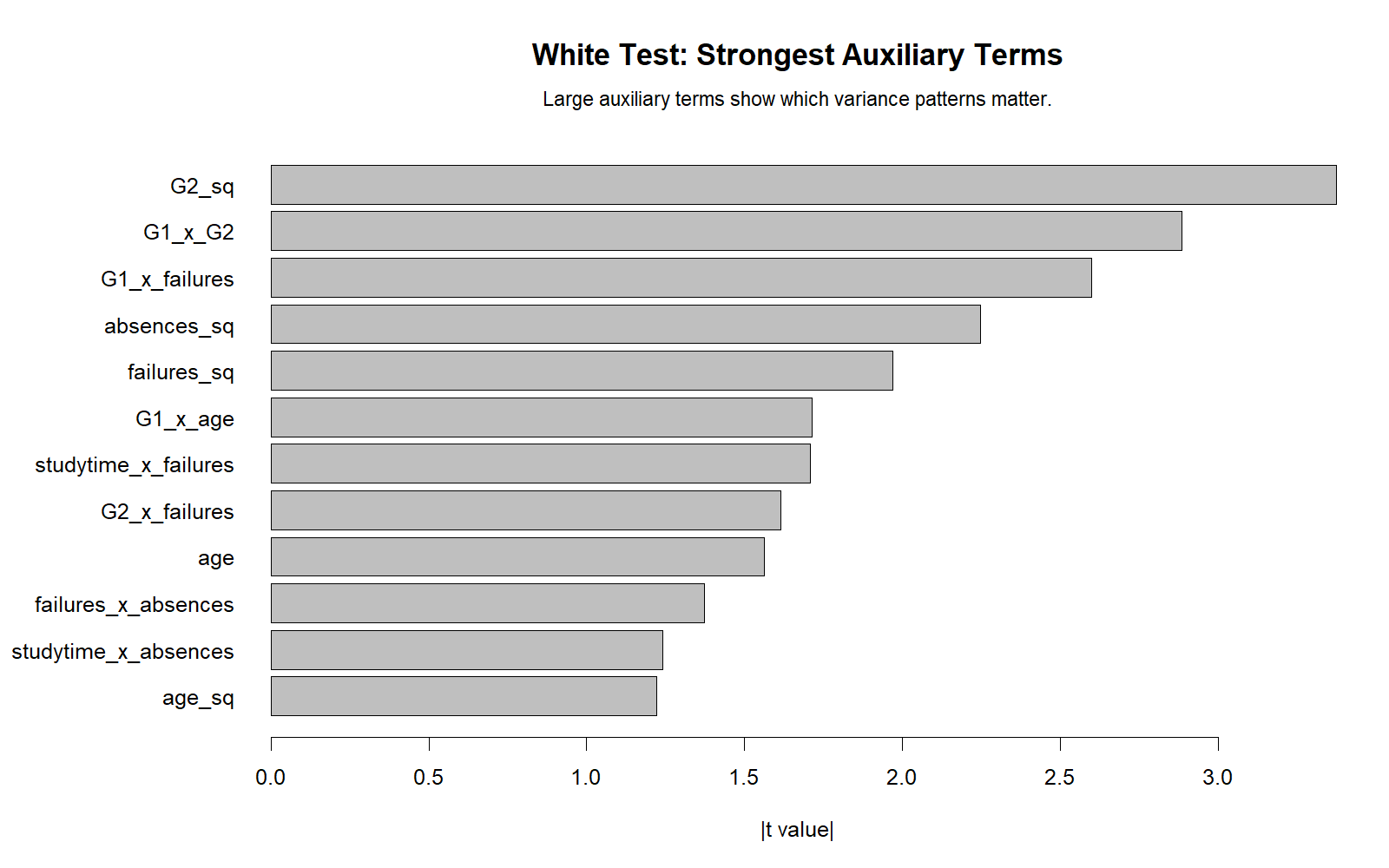
The R auxiliary-term chart confirms that variance structure is most strongly connected with grade-related squared and interaction terms such as G2_sq, G1_x_G2 and G1_x_failures. This supports the interpretation that heteroskedasticity is related to nonlinear and interaction patterns in the prediction structure.
6. R Residual Distribution
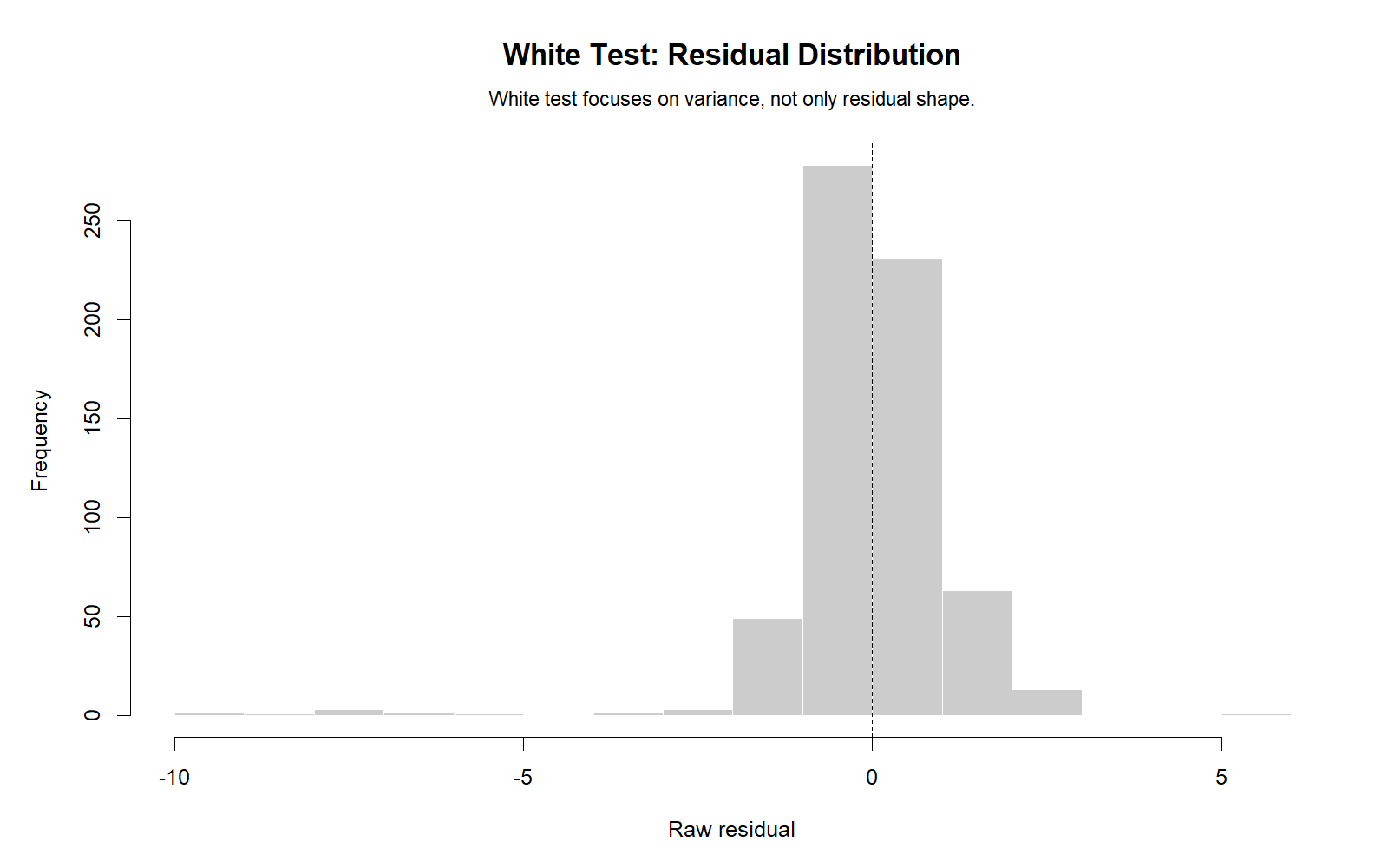
The R residual histogram confirms that residuals are centered near zero but have tail irregularities. This supports the broader diagnostic story while keeping the main focus on variance. The White Test result is about heteroskedasticity, not merely residual normality.
7. R Base and Auxiliary Model Fit
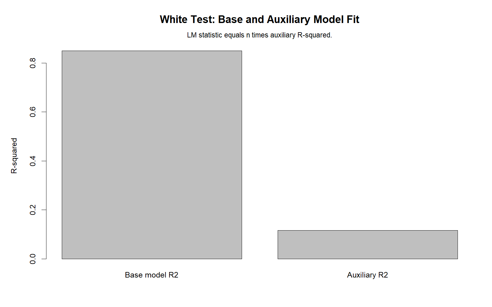
The R model-fit chart confirms that the base regression fit is strong, while the auxiliary regression still explains enough squared residual variation to trigger a significant White Test. The final interpretation remains unchanged: the regression has strong predictive power, but the residual variance is not constant.
SPSS Output Interpretation
The SPSS output PDF contains the base regression, auxiliary regression, residual descriptives and residual normality/spread context. SPSS confirms that the base regression is strong and that the auxiliary regression for squared residuals is statistically significant.
Base Regression in SPSS
The SPSS base regression used G3 as the dependent variable and entered G1, G2, studytime, failures, absences and age as predictors. The model summary shows R = .922, R² = .851, adjusted R² = .849 and a standard error of estimate of 1.254. The ANOVA table shows F(6, 642) = 609.353, p < .001. This means the base regression is statistically significant and explains a large amount of variation in G3.
Residual Statistics in SPSS
The SPSS residual statistics show predicted values ranging from about .31 to 19.58. Raw residuals range from -9.045 to 5.817, with mean approximately 0 and standard deviation about 1.249. The residual range is wide enough to justify visual residual diagnostics. The standardized residual minimum of -7.210 also shows that some cases are far from the fitted line.
White Auxiliary Regression in SPSS
The SPSS auxiliary regression used resid_sq as the dependent variable. The final auxiliary model included predictors, squared predictors and interaction terms. The final model summary shows R = .341, R² = .116 and adjusted R² = .078. The ANOVA table for the final auxiliary model shows F(27, 621) = 3.030, p < .001. This supports the White Test conclusion that the squared residuals are related to the auxiliary terms.
Important Auxiliary Terms in SPSS
| Auxiliary term | SPSS t value | SPSS p-value | Interpretation |
|---|---|---|---|
| G2_sq | -3.376 | .001 | The squared G2 term is strongly related to squared residuals. |
| G1_x_G2 | 2.885 | .004 | The interaction of G1 and G2 contributes to variance structure. |
| G1_x_failures | 2.599 | .010 | The combination of G1 and failures is related to residual variance. |
| absences_sq | 2.248 | .025 | Nonlinear absence patterns help explain squared residuals. |
| failures_sq | -1.968 | .049 | The squared failures term is borderline significant in the final auxiliary model. |
Residual Normality and Spread Context
The SPSS Explore output shows that raw residuals have skewness = -2.864 and kurtosis = 18.667. Squared residuals have skewness = 8.651 and kurtosis = 80.487. Both Kolmogorov-Smirnov and Shapiro-Wilk tests are significant for residuals and squared residuals. This does not replace the White Test, but it confirms that residual behavior is not simple and normal-looking. For residual normality interpretation, compare this with Kolmogorov-Smirnov Test and Lilliefors Test.
How to Run White Test in Python, R, SPSS and Excel
Python Method
In Python, the easiest method is to fit an OLS model with statsmodels, extract residuals and use the White Test diagnostic function. The following code structure matches the logic used for this post.
import pandas as pd
import statsmodels.api as sm
from statsmodels.stats.diagnostic import het_white

df = pd.read_csv("student-por.csv", sep=";")

y = df["G3"]
X = df[["G1", "G2", "studytime", "failures", "absences", "age"]]
X = sm.add_constant(X)

model = sm.OLS(y, X).fit()

white_lm, white_lm_p, white_f, white_f_p = het_white(model.resid, model.model.exog)

print("Base R-squared:", model.rsquared)
print("White LM statistic:", white_lm)
print("White LM p-value:", white_lm_p)
print("White F statistic:", white_f)
print("White F p-value:", white_f_p)

if white_lm_p < 0.05:
    print("Reject H0: evidence of heteroskedasticity")
else:
    print("Fail to reject H0: no strong evidence of heteroskedasticity")
R Method
In R, you can manually build a White-style auxiliary regression by modeling squared residuals with predictors, squared predictors and interaction terms.
df <- read.csv("student-por.csv", sep = ";")

base_model <- lm(G3 ~ G1 + G2 + studytime + failures + absences + age, data = df)

df$resid_G3 <- resid(base_model)
df$resid_sq <- df$resid_G3^2

aux_model <- lm(
  resid_sq ~ G1 + G2 + studytime + failures + absences + age +
    I(G1^2) + I(G2^2) + I(studytime^2) + I(failures^2) + I(absences^2) + I(age^2) +
    G1:G2 + G1:studytime + G1:failures + G1:absences + G1:age +
    G2:studytime + G2:failures + G2:absences + G2:age +
    studytime:failures + studytime:absences + studytime:age +
    failures:absences + failures:age + absences:age,
  data = df
)

n <- nobs(aux_model)
aux_r2 <- summary(aux_model)$r.squared
df_white <- length(coef(aux_model)) - 1
lm_stat <- n * aux_r2
p_value <- pchisq(lm_stat, df = df_white, lower.tail = FALSE)

print(summary(base_model))
print(summary(aux_model))
print(lm_stat)
print(p_value)
SPSS Method
In SPSS, run the base regression first, save predicted values and residuals, compute squared residuals, compute squared predictors and interactions, then run the auxiliary regression with resid_sq as the dependent variable.
REGRESSION
  /DEPENDENT G3
  /METHOD=ENTER G1 G2 studytime failures absences age
  /SAVE PRED(pred_G3) RESID(resid_G3).

COMPUTE resid_sq = resid_G3 ** 2.
COMPUTE G1_sq = G1 ** 2.
COMPUTE G2_sq = G2 ** 2.
COMPUTE studytime_sq = studytime ** 2.
COMPUTE failures_sq = failures ** 2.
COMPUTE absences_sq = absences ** 2.
COMPUTE age_sq = age ** 2.

COMPUTE G1_x_G2 = G1 * G2.
COMPUTE G1_x_studytime = G1 * studytime.
COMPUTE G1_x_failures = G1 * failures.
COMPUTE G1_x_absences = G1 * absences.
COMPUTE G1_x_age = G1 * age.
COMPUTE G2_x_studytime = G2 * studytime.
COMPUTE G2_x_failures = G2 * failures.
COMPUTE G2_x_absences = G2 * absences.
COMPUTE G2_x_age = G2 * age.
COMPUTE studytime_x_failures = studytime * failures.
COMPUTE studytime_x_absences = studytime * absences.
COMPUTE studytime_x_age = studytime * age.
COMPUTE failures_x_absences = failures * absences.
COMPUTE failures_x_age = failures * age.
COMPUTE absences_x_age = absences * age.
EXECUTE.

REGRESSION
  /DEPENDENT resid_sq
  /METHOD=ENTER G1 G2 studytime failures absences age
    G1_sq G2_sq studytime_sq failures_sq absences_sq age_sq
    G1_x_G2 G1_x_studytime G1_x_failures G1_x_absences G1_x_age
    G2_x_studytime G2_x_failures G2_x_absences G2_x_age
    studytime_x_failures studytime_x_absences studytime_x_age
    failures_x_absences failures_x_age absences_x_age.

OUTPUT EXPORT
  /CONTENTS EXPORT=ALL
  /PDF DOCUMENTFILE="D:\DATA ANALYSIS\B Normality and Assumption Tests\White Test\SPSS_Output\White-Test-SPSS-Output.pdf".
Excel Method
Excel does not have a one-click White Test button, but the method is still possible with the Data Analysis ToolPak. First run the base regression and save residuals. Then square the residuals. Next create columns for squared predictors and interaction terms. Finally regress squared residuals on those auxiliary columns and calculate the LM statistic.
| Excel step | Formula or action | Explanation |
|---|---|---|
| Run base regression | Data Analysis → Regression | Use G3 as Y and G1, G2, studytime, failures, absences and age as X. |
| Save residuals | Check residual output | Excel creates residual values from the base regression. |
| Square residuals | =Residual_Cell^2 | This becomes the dependent variable for the auxiliary regression. |
| Create squared predictors | =G1_Cell^2, =G2_Cell^2 | Repeat for all numeric predictors. |
| Create interaction terms | =G1_Cell*G2_Cell | Repeat for required predictor pairs. |
| Run auxiliary regression | Y = squared residuals; X = auxiliary terms | Record the auxiliary R². |
| Calculate LM statistic | =N*Auxiliary_R2 | For this post, approximately 649 × 0.1164. |
| Calculate p-value | =CHISQ.DIST.RT(LM, df) | Use df equal to the number of auxiliary predictors. |
How to Report the White Test
A good White Test report should include the null hypothesis, alternative hypothesis, base model context, auxiliary regression result, p-value decision and practical conclusion. It should also explain what to do after detecting heteroskedasticity.
APA-Style Report Example
A White Test for heteroskedasticity was conducted on the residuals from an OLS regression predicting G3 final grade from G1, G2, studytime, failures, absences and age. The null hypothesis stated that the residual variance was constant. The auxiliary regression produced R² = 0.1164, and the White LM p-value was 1.753e-06. Because the p-value was below .05, the null hypothesis of homoscedasticity was rejected. The result indicates significant heteroskedasticity, so robust standard errors should be considered when reporting coefficient significance.
Do not report only the p-value. A complete report should explain that the White Test is about residual variance, not about the overall regression fit. In this example, the base regression has high R², but heteroskedasticity is still present.
What to Do After a Significant White Test
| Option | When useful | Reporting note |
|---|---|---|
| Use robust standard errors | When coefficients are still meaningful but standard errors may be biased. | Report heteroskedasticity-robust standard errors. |
| Transform the dependent variable | When residual spread increases with the outcome scale. | Compare transformed and original models carefully. |
| Add missing nonlinear terms | When plots suggest curvature or omitted nonlinear structure. | Model misspecification can look like heteroskedasticity. |
| Check influential cases | When a few observations produce very large squared residuals. | Do not delete cases automatically; diagnose them first. |
| Compare related tests | When you need confirmation from another diagnostic. | Use Goldfeld-Quandt or group variance tests where appropriate. |
Common Mistakes When Interpreting the White Test
| Mistake | Why it is wrong | Correct approach |
|---|---|---|
| Calling White Test a normality test | White Test checks variance, not residual normality. | Use Q-Q plots and normality tests for residual shape. |
| Writing p = .000 | A p-value is not exactly zero. | Write p < .001 or use the precise value such as 1.753e-06. |
| Ignoring plots because the base R² is high | High predictive fit does not guarantee constant variance. | Report both model fit and diagnostic assumptions. |
| Thinking heteroskedasticity means the model is useless | The coefficients may still be useful, but standard errors can be unreliable. | Consider robust standard errors or model improvement. |
| Using too many auxiliary terms in a small dataset | The auxiliary regression can become unstable. | Use White Test carefully and check degrees of freedom. |
Downloads and Resources
The following hosted resources support this White Test guide. The SPSS PDF contains the regression output, auxiliary regression and residual diagnostic context. The chart links show the Python and R visual outputs used in the interpretation sections above.
SPSS Output PDF
White Test SPSS output with base regression, auxiliary regression and residual diagnostics.
Python Decision Chart
White LM p-value decision chart comparing p-value with alpha threshold.
Python Auxiliary Terms Chart
Top auxiliary terms ranked by absolute t value.
R Model Fit Chart
R validation chart comparing base model R² and auxiliary R².
External References
FAQs About White Test
What is the White Test?
The White Test is a regression diagnostic test for heteroskedasticity. It checks whether residual variance is constant or whether squared residuals can be explained by predictors, squared predictors and interaction terms.
What is the null hypothesis of the White Test?
The null hypothesis is that the residual variance is constant. In other words, H0: homoscedasticity. If the p-value is below alpha, reject the null hypothesis.
What is the alternative hypothesis of the White Test?
The alternative hypothesis is that the residual variance is not constant. In other words, H1: heteroskedasticity.
How do I interpret p = 1.753e-06 in the White Test?
A p-value of 1.753e-06 is much smaller than .05. Therefore, reject the null hypothesis of constant variance. In report form, you can also write p < .001.
Is White Test the same as Breusch-Pagan test?
No. Both tests check heteroskedasticity, but the White Test is more general because it can include original predictors, squared predictors and interaction terms. The Breusch-Pagan test is usually simpler and often tests a more direct relationship between variance and predictors.
Does a significant White Test mean my regression is useless?
No. It means the constant variance assumption is violated. The coefficients may still be useful, but ordinary standard errors and p-values may be unreliable. Robust standard errors are commonly used after detecting heteroskedasticity.
Can I do White Test in Excel?
Yes. Run the base regression, save residuals, square the residuals, create squared predictor and interaction columns, run an auxiliary regression and calculate LM = n × auxiliary R². Then use CHISQ.DIST.RT to calculate the p-value.
Is White Test a normality test?
No. White Test checks constant variance. For residual normality, use a Q-Q plot, P-P plot, Shapiro-Wilk, Kolmogorov-Smirnov or related normality tests.

