
Equal Group Sizes, One-Way ANOVA, Balanced Sampling, F Statistic, Residuals and Effect Size
Balanced ANOVA: Formula, Equal Group Sizes, SPSS, Python, R and Excel Guide
Balanced ANOVA is an ANOVA design where every group contributes the same number of observations. In this guide, the original studytime groups were unequal, so a balanced ANOVA sample was created by using 35 cases from each studytime group. The balanced sample compares G3 final grade across four studytime groups using Python charts, R validation charts, SPSS output, sum of squares, F statistic, residual histogram, effect size summary, formulas, code blocks and APA reporting.
Quick Answer: Balanced ANOVA Result
The worked Balanced ANOVA example compares G3 final grade across four studytime groups after equalizing the group sizes. The original dataset was unbalanced, with group sizes around 212, 305, 97 and 35. The balanced ANOVA sample uses 35 cases in each group, so the final balanced sample contains 140 cases.
The balanced group means are close to one another: 12.229 for studytime group 1, 13.143 for group 2, 12.886 for group 3 and 13.057 for group 4. The F distribution chart shows observed F = 1.11 and critical F = 2.67. Because the observed F statistic is below the critical value, the balanced ANOVA does not show a statistically significant group mean difference at the .05 level.
Final interpretation: After balancing the studytime groups to 35 cases each, the ANOVA result becomes small and non-significant. The group means remain in the same general grade range, the between-group sum of squares is much smaller than the within-group sum of squares, and the observed F value does not cross the critical F boundary.
Important reporting point: Balanced ANOVA changes the sample structure. It removes the influence of unequal group sizes but may also reduce statistical power because many observations from larger groups are not used. In this example, balancing produces a cleaner equal-size comparison, but the result is weaker than the full unbalanced ANOVA pattern.
Table of Contents
- What Is Balanced ANOVA?
- Balanced ANOVA Formula
- Null and Alternative Hypothesis
- Dataset and Balanced Sampling Used
- Python Chart-by-Chart Interpretation
- R Chart-by-Chart Validation
- SPSS Output Interpretation
- SPSS, R, Python and Excel Workflows
- Code Blocks for Balanced ANOVA
- APA Reporting Wording
- Common Mistakes
- When to Use Balanced ANOVA
- Downloads and Resources
- Related Guides
- FAQs
What Is Balanced ANOVA?
Balanced ANOVA is an ANOVA design where every group has the same sample size. In a one-way balanced ANOVA, each category of the grouping factor contributes an equal number of observations. This makes the design easier to interpret because each group has the same weight in the mean comparison.
In this example, the original studytime groups were not equal. Studytime group 2 had the largest number of observations, and group 4 had the smallest number of observations. The balanced ANOVA sample used the smallest group size as the target, so all four groups were reduced to 35 observations each.
A balanced ANOVA is useful when the analyst wants a clean equal-size comparison. It can reduce the dominance of very large groups, but it also discards data from larger groups when balancing is done by subsampling. That is why the balanced result should be interpreted as a sensitivity check or equal-size comparison, not automatically as a replacement for the full dataset result.
Simple definition: Balanced ANOVA compares group means after making the group sizes equal. In this example, each studytime group contributes 35 cases, so the ANOVA compares four equally sized groups.
Balanced ANOVA is closely related to ANOVA Assumptions, ANOVA Effect Size, ANOVA in Python, ANOVA in R, ANOVA in SPSS, Effect Size, P Value, and Null and Alternative Hypothesis.
Balanced ANOVA Formula
A one-way balanced ANOVA model can be written as:
Here, Yij is the observed G3 score for student j in studytime group i, μ is the grand mean, τi is the group effect, and εij is the residual error. The balanced design means that every group has the same number of observations.
Equal Group Size Condition
This condition is the defining feature of the example. The original group sizes were unequal, but the balanced sample uses 35 observations from each studytime group.
ANOVA F Statistic
The F statistic compares between-group mean variation with within-group variation. In the balanced output, the observed F value is 1.11, while the critical F value is 2.67. Since the observed value is lower than the critical boundary, the balanced ANOVA does not reject the null hypothesis at α = .05.
Eta Squared Formula
Eta squared measures the proportion of total variation explained by the group factor. In this balanced ANOVA, eta squared is .0239, meaning studytime explains only about 2.39% of the total G3 variation in the balanced sample.
| Balanced ANOVA Term | Value in This Example | Meaning | Interpretation |
|---|---|---|---|
| Original group sizes | 212, 305, 97, 35 | The full dataset is unbalanced. | Larger groups would have more representation in the full sample. |
| Balanced group size | 35 per group | Each group contributes equally. | The balanced sample contains 140 cases. |
| Observed F | 1.11 | Between-group variation divided by within-group variation. | Below the critical F value. |
| Critical F | 2.67 | Decision boundary at α = .05. | The observed F does not cross the boundary. |
| Eta squared | .0239 | Percent variance explained by studytime. | Small explained variance in the balanced sample. |
| Cohen’s f | .1566 | Standardized ANOVA effect size. | Small-to-moderate practical magnitude. |
Null and Alternative Hypothesis for Balanced ANOVA
The balanced ANOVA tests whether mean G3 is equal across the four equally sized studytime groups. The null hypothesis says that all balanced group means are equal. The alternative hypothesis says that at least one balanced group mean differs.
| Hypothesis | Statement | Meaning for This Balanced ANOVA |
|---|---|---|
| Null hypothesis | H0: μ1 = μ2 = μ3 = μ4 | All balanced studytime groups have the same mean G3 score. |
| Alternative hypothesis | H1: at least one group mean differs | At least one balanced studytime group has a different mean G3 score. |
| Decision evidence | Observed F = 1.11 and critical F = 2.67 | The observed F is below the rejection boundary. |
| Effect-size evidence | η² = .0239, ω² = .0024, Cohen’s f = .1566 | The practical effect is small in the balanced sample. |
Decision for this example: The balanced ANOVA does not reject the null hypothesis at the .05 level. The balanced studytime groups have similar G3 means, and the effect-size values show that studytime explains only a small part of G3 variation after balancing the sample.
Dataset and Balanced Sampling Used
The worked example uses a student performance dataset. The dependent variable is G3 final grade, and the grouping factor is studytime. The original data are unbalanced because the four studytime groups do not have equal sample sizes.
The balanced ANOVA sample uses the smallest original group size as the target sample size. Since studytime group 4 has 35 cases, the balanced workflow uses 35 cases from each studytime group. This creates a final balanced sample of 140 cases.
| Variable or Output | Role | Value or Meaning | Why It Matters |
|---|---|---|---|
| G3 | Dependent variable | Final grade | Numeric outcome compared across groups. |
| studytime | Grouping factor | Four groups | Defines the balanced ANOVA groups. |
| Original N | Full dataset group sizes | 212, 305, 97, 35 | Shows the original design is unbalanced. |
| Balanced N | Equalized group sizes | 35, 35, 35, 35 | Creates equal group weight. |
| Residuals | Model errors | Observed G3 minus group mean | Used for diagnostic histogram. |
| Effect size | Practical magnitude | η² = .0239 | Shows the balanced effect is small. |
Balanced sampling should be interpreted together with Descriptive Statistics, Mean Median and Mode, Standard Deviation, Variance, Standard Error, Confidence Interval, Effect Size, and Statistical Power.
Python Chart-by-Chart Interpretation
The Python charts below show the balanced ANOVA workflow from sample balancing to final interpretation. They explain the original versus balanced group sizes, balanced group means, balanced boxplot, sum of squares, F distribution, residual histogram and effect size summary.
Python Chart 1: Original vs Balanced Group Sizes
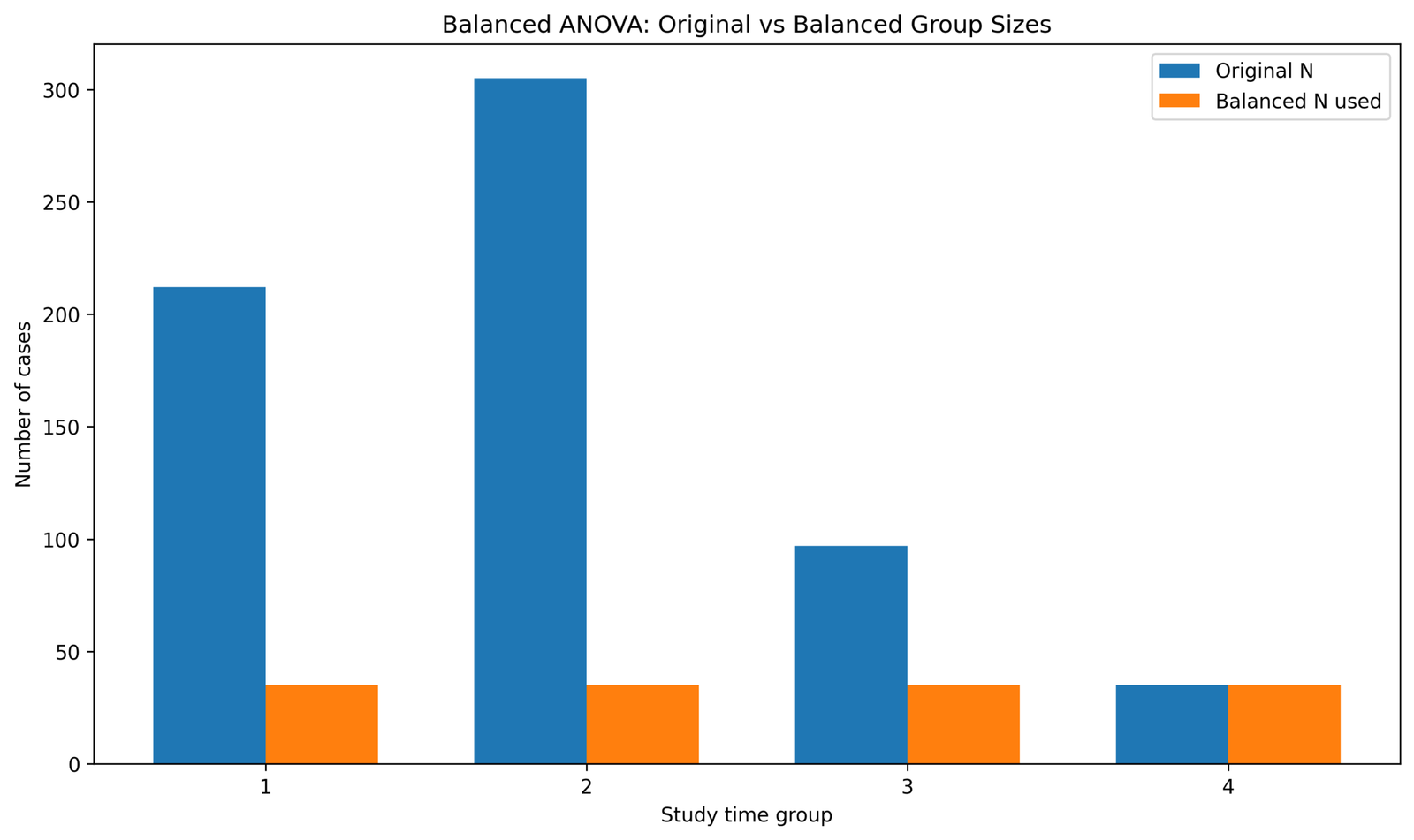
This chart shows why a balanced ANOVA workflow was needed. The original group sizes are clearly unequal: studytime group 2 is the largest group, group 1 is also large, group 3 is smaller, and group 4 is the smallest. The balanced bars show that each group was reduced to the same sample size of 35 cases.
The chart is important because it shows that balancing is not a statistical test by itself. It is a sampling decision before the ANOVA is run. The equal orange bars mean that every studytime group receives the same weight in the balanced ANOVA comparison.
In the final report, this chart should be used to explain the difference between the full unbalanced dataset and the balanced analysis sample. The result should be described as a balanced-sample ANOVA, not as the full-data ANOVA.
Python Chart 2: Balanced Group Means with 95% Confidence Intervals
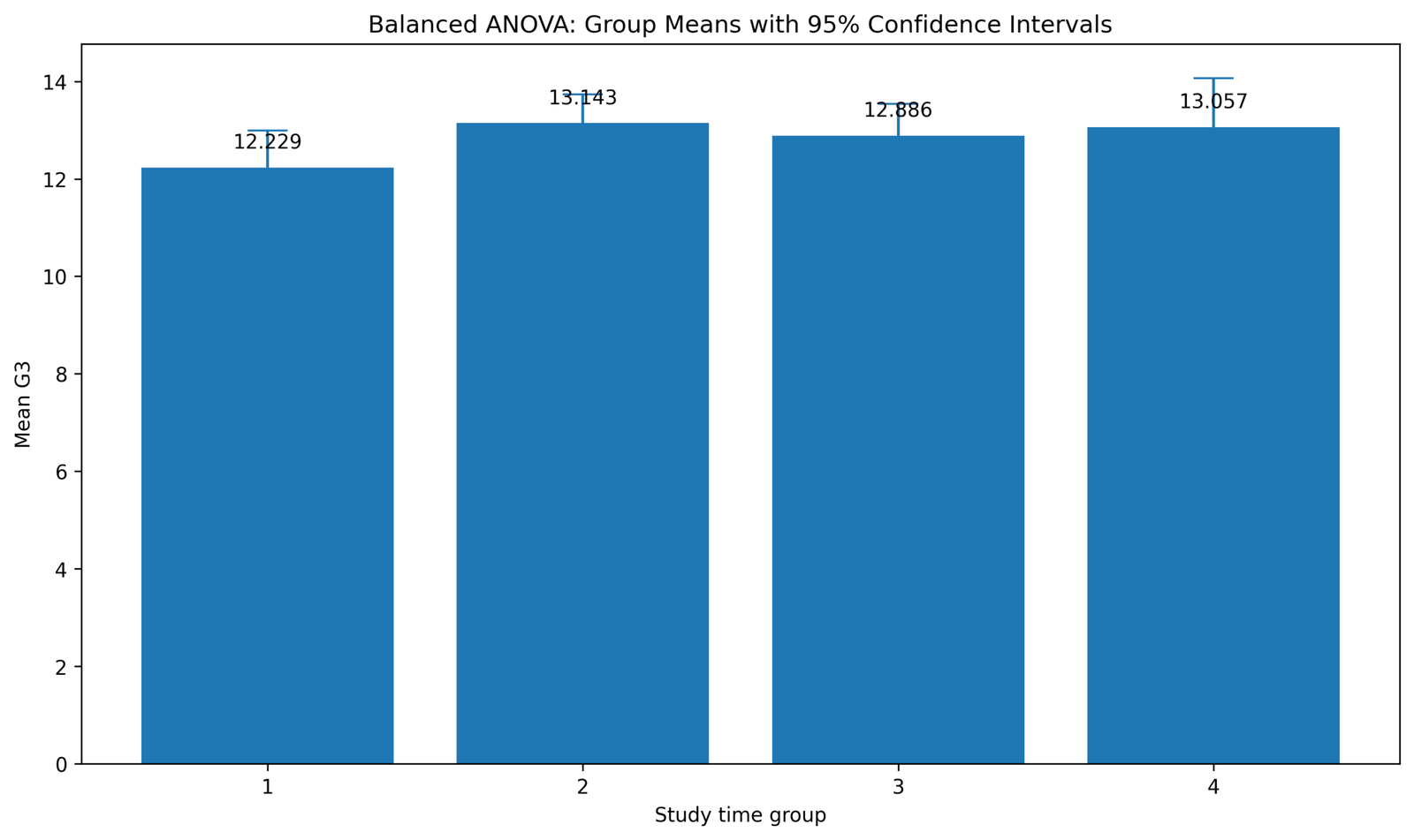
This chart shows the balanced mean G3 values after every studytime group was set to 35 cases. The means are 12.229 for group 1, 13.143 for group 2, 12.886 for group 3 and 13.057 for group 4.
The group means are close together. Group 2 has the highest mean, group 1 has the lowest mean, and groups 3 and 4 sit between or near the top. The difference between the lowest and highest balanced means is less than one G3 point.
This chart explains why the balanced ANOVA F statistic is small. The group means do not separate strongly after balancing, so the between-group variation is limited. The result is a much weaker group pattern than an analysis where large unequal groups dominate the comparison.
Python Chart 3: Balanced Boxplot of G3 by Studytime Group
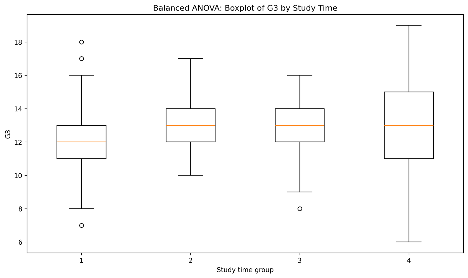
This boxplot shows the distribution of G3 inside each balanced studytime group. The medians are similar across groups, with group 1 centered around 12 and the other groups centered around 13. The boxes overlap strongly, which supports the non-significant ANOVA decision.
Group 1 contains a few visible outliers, including low and high values. Group 3 has a low point near 8, and group 4 has a wider spread that reaches from about 6 to 19. The group centers are not far apart, but the within-group spread remains visible.
For balanced ANOVA reporting, this chart supports a practical conclusion: the balanced groups do not show a strong separation in G3 scores. The distributions overlap enough that the observed mean differences are small compared with within-group variation.
Python Chart 4: Sum of Squares Decomposition
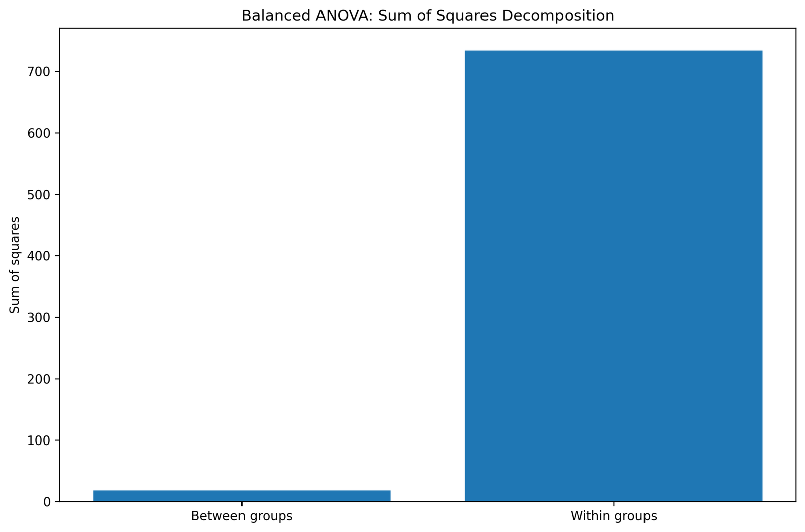
This chart separates total variation into between-group and within-group components. The between-group sum of squares is very small, while the within-group sum of squares is much larger. This means most G3 variation remains inside the studytime groups rather than being explained by differences between studytime groups.
The small between-group bar matches the group mean chart. Since the four balanced means are close together, there is not much explained group variation. The large within-group bar shows that individual scores still vary substantially within each studytime group.
In the final article, this chart should be used to explain the F result. The observed F statistic is small because the between-group mean square is not large enough compared with the within-group mean square.
Python Chart 5: F Statistic Distribution Curve
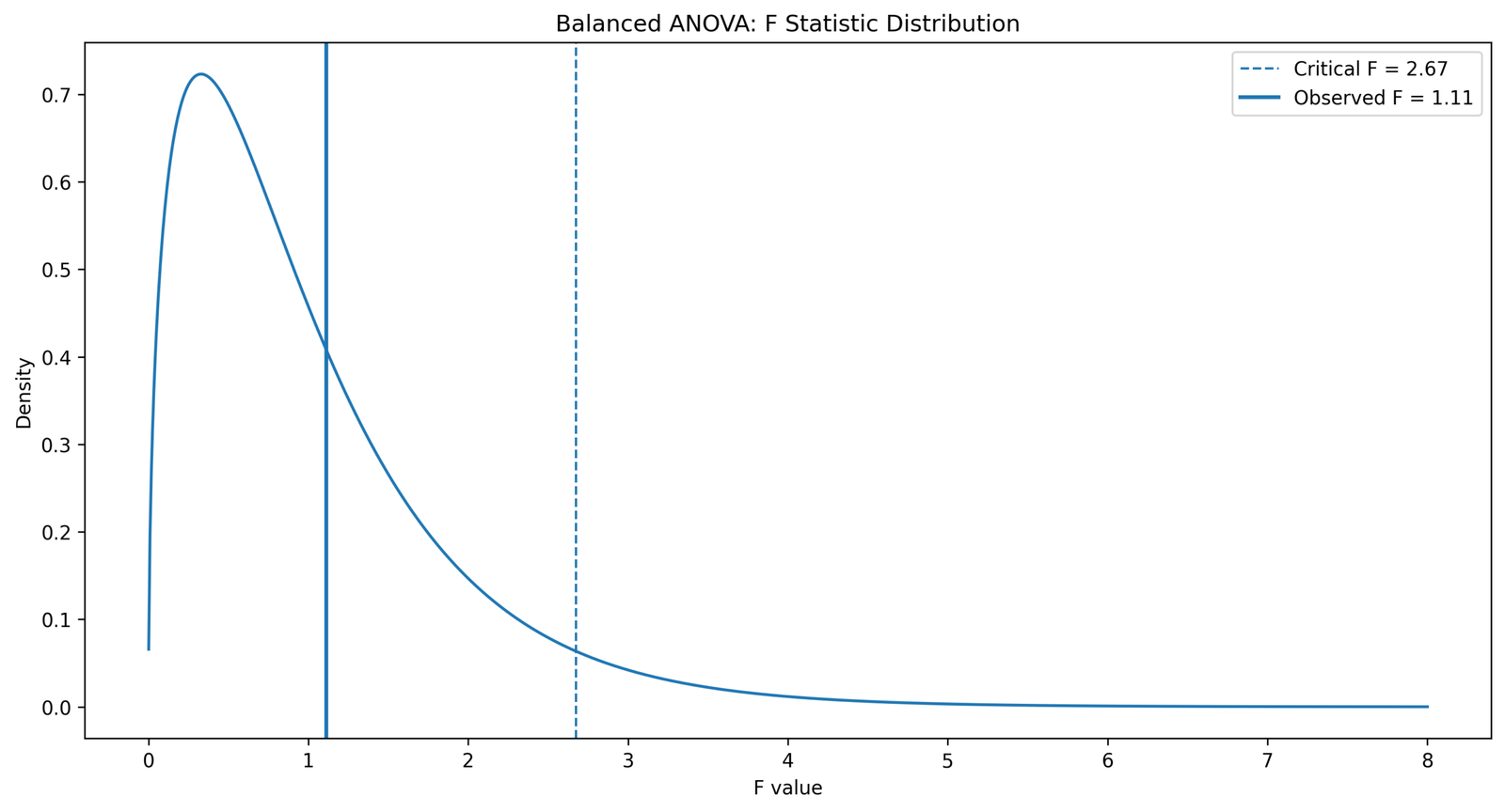
This chart shows the balanced ANOVA F distribution. The observed F statistic is 1.11, while the critical F value is 2.67. The observed F line is to the left of the critical F line.
Because the observed F value does not reach the critical boundary, the balanced ANOVA does not reject the null hypothesis at the .05 level. The result means the balanced studytime group means are not different enough relative to within-group variation.
This chart should be used as the main decision visual. It shows the statistical result more clearly than a table alone: the group effect is present numerically, but it is not strong enough to be declared statistically significant in the balanced sample.
Python Chart 6: Balanced ANOVA Residual Histogram
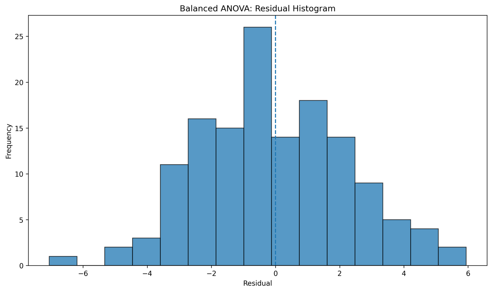
This histogram shows the residuals from the balanced ANOVA model. Most residuals are clustered near zero, which means many observed G3 scores are reasonably close to their balanced group mean.
The residuals extend to about -7 on the negative side and about 6 on the positive side. The shape is not perfectly normal, but it is centered around zero and does not show a single extreme tail dominating the entire plot.
In reporting, this chart supports a moderate diagnostic statement. The balanced ANOVA residuals are centered near zero, but the distribution still shows real within-group variation. This is consistent with the large within-group sum of squares and the non-significant F result.
Python Chart 7: Balanced ANOVA Effect Size Summary
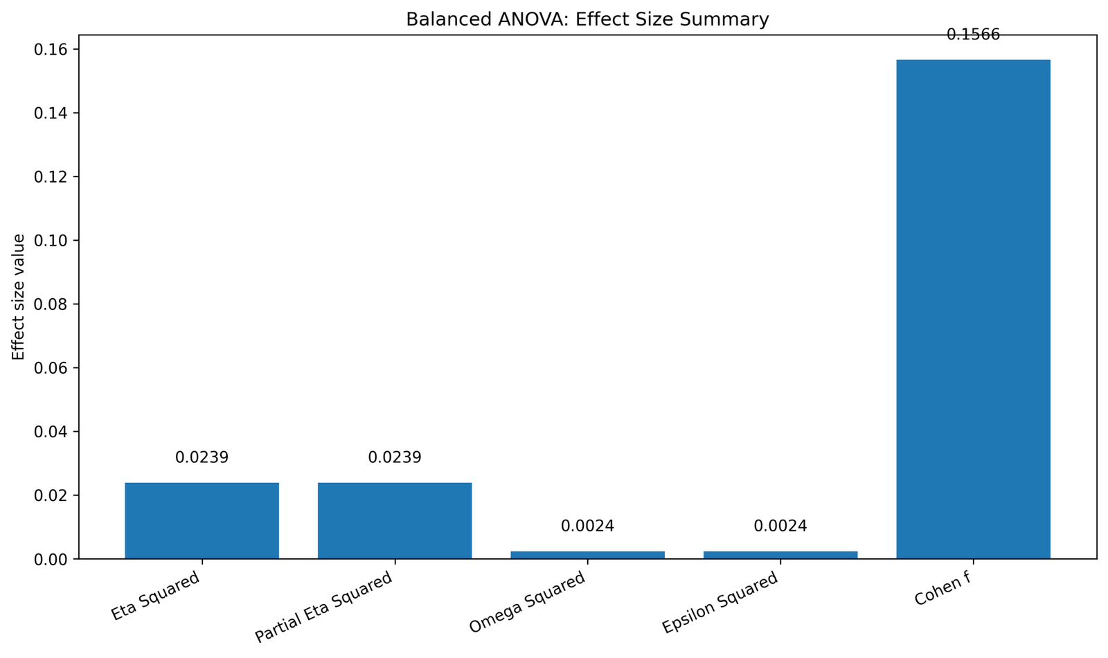
This effect size chart shows that eta squared and partial eta squared are both 0.0239. Omega squared and epsilon squared are both 0.0024. Cohen’s f is 0.1566.
The effect size values confirm that the balanced studytime effect is small. Eta squared means that studytime explains only about 2.39% of the total variation in G3 in the balanced sample. Omega squared and epsilon squared are even smaller because they adjust the estimate downward.
In the final report, this chart should be used after the F statistic. The correct interpretation is that the balanced ANOVA did not find a statistically significant group difference, and the effect size is small in practical terms.
R Chart-by-Chart Validation
The R validation charts repeat the same balanced ANOVA workflow in a second software environment. The R charts confirm the equal group sizes, similar group means, overlapping boxplots, small between-group variation, non-significant F decision, centered residuals and small effect-size values.
R Chart 1: Original vs Balanced Group Sizes
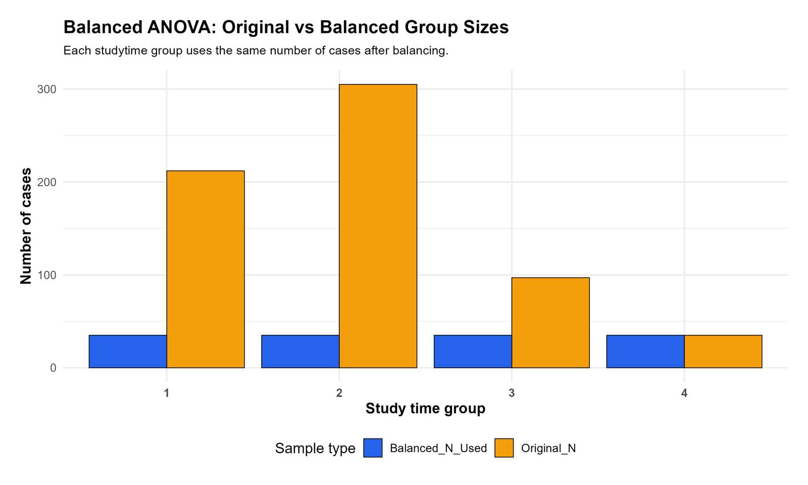
This R chart confirms the same sampling structure shown in Python. The original studytime groups are unequal, while the balanced sample uses the same number of observations from each group.
The equal balanced bars show that the ANOVA validation is based on 35 cases per group. This confirms that R is checking the same balanced design, not the original unbalanced dataset.
In reporting, this chart should be used to verify the analysis design. It shows that the balanced result is based on equal group representation and therefore answers a balanced-sample question.
R Chart 2: Balanced Group Means with 95% Confidence Intervals
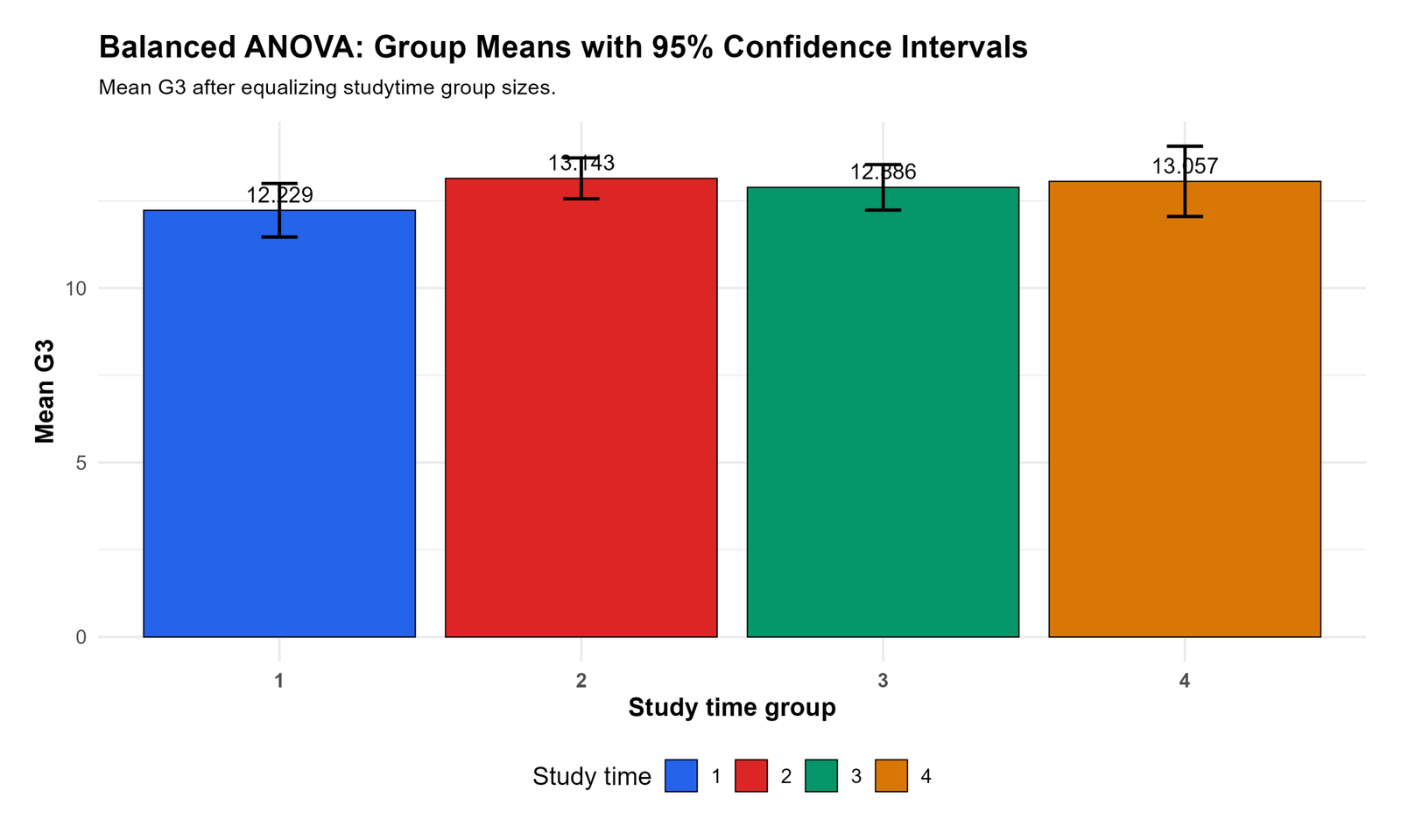
This R chart labels the balanced group means as 12.229, 13.143, 12.886 and 13.057. The values match the Python chart and confirm that the balanced groups are close together.
The confidence intervals overlap visually. This supports the non-significant ANOVA decision because the group mean differences are not large compared with the uncertainty and within-group variation.
In the final report, this R chart confirms the direction and size of the balanced mean pattern. Group 2 is highest, group 1 is lowest, but the separation is not large enough to produce a significant balanced ANOVA result.
R Chart 3: Balanced Boxplot of G3 by Studytime Group
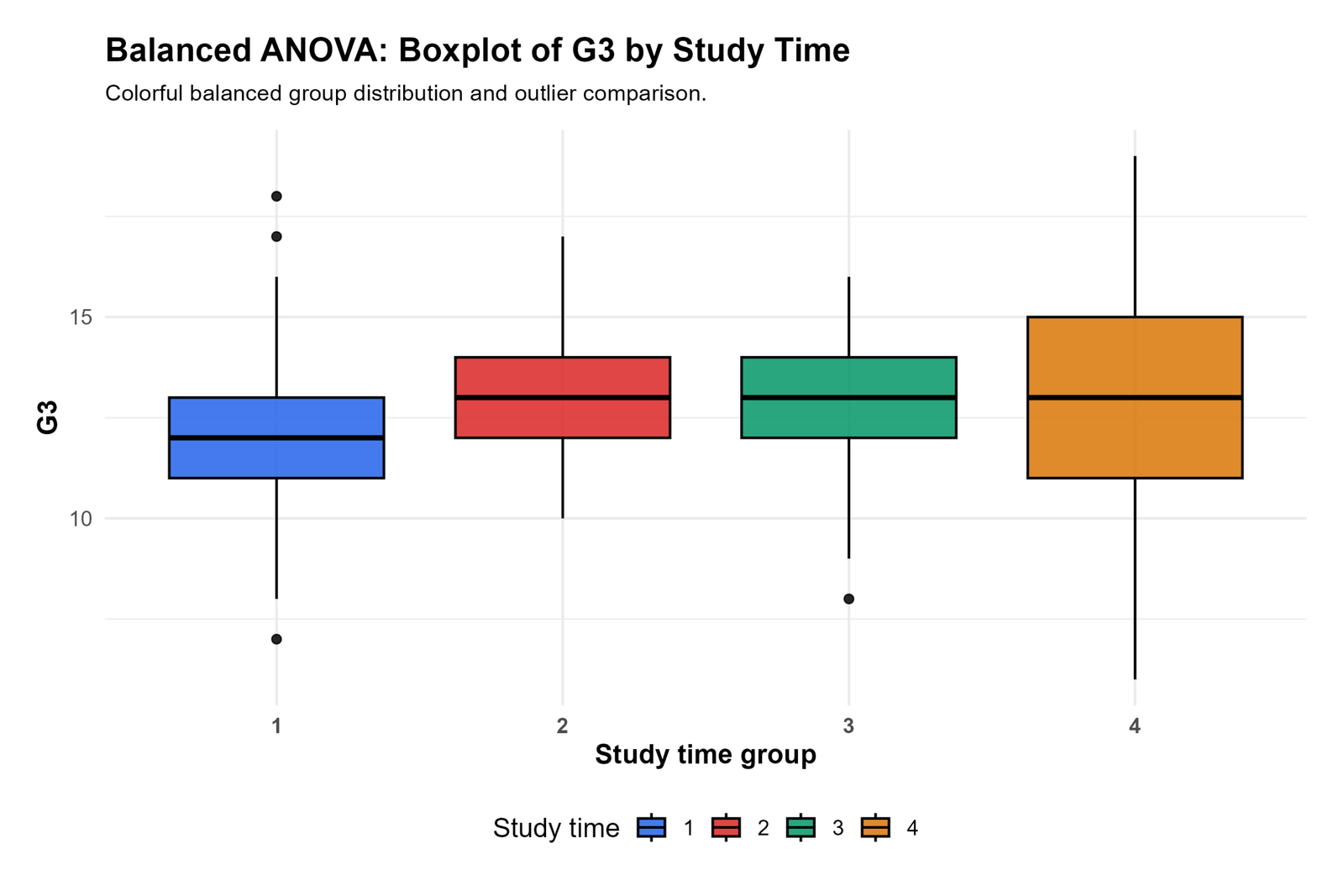
The R boxplot confirms that the balanced group distributions overlap strongly. The medians are close, and the boxes are not separated into clearly different score regions.
Group 4 shows a relatively wide range, while group 1 includes visible outlier points. These distribution features explain why within-group variation remains large even after balancing the group sizes.
In reporting, this chart supports the conclusion that balanced sampling did not create a strong group separation. The group means differ slightly, but individual G3 scores still vary considerably within each group.
R Chart 4: Sum of Squares Decomposition
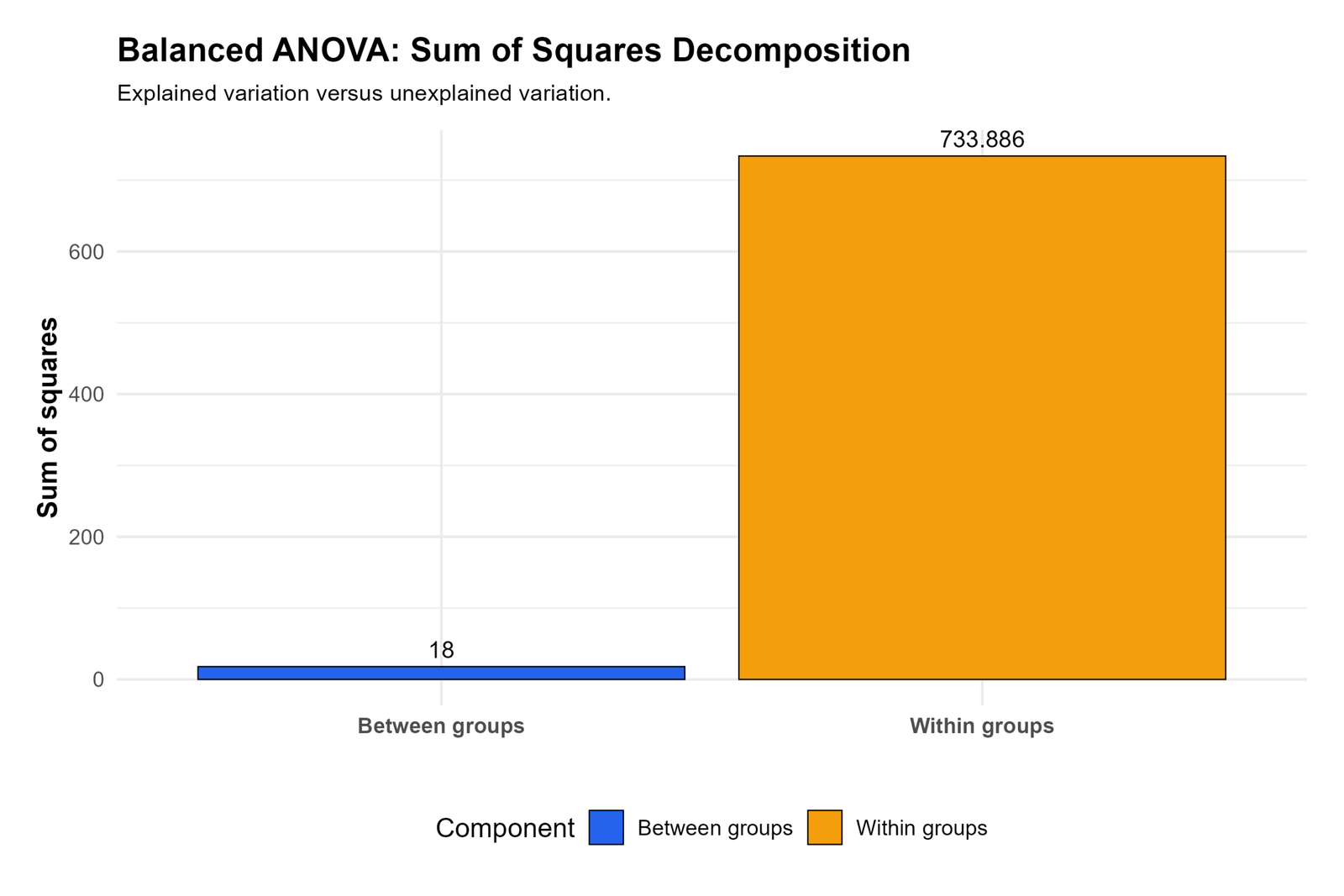
This R chart confirms that within-group variation is much larger than between-group variation. The studytime group effect explains only a small part of the total G3 variation in the balanced sample.
The chart matches the small eta squared value. Since eta squared is calculated from the between-group sum of squares divided by the total sum of squares, a small between-group bar naturally produces a small explained-variance result.
In reporting, this chart validates the core ANOVA logic. The balanced F statistic is small because the explained group variation is weak compared with the unexplained within-group variation.
R Chart 5: F Statistic Distribution Curve
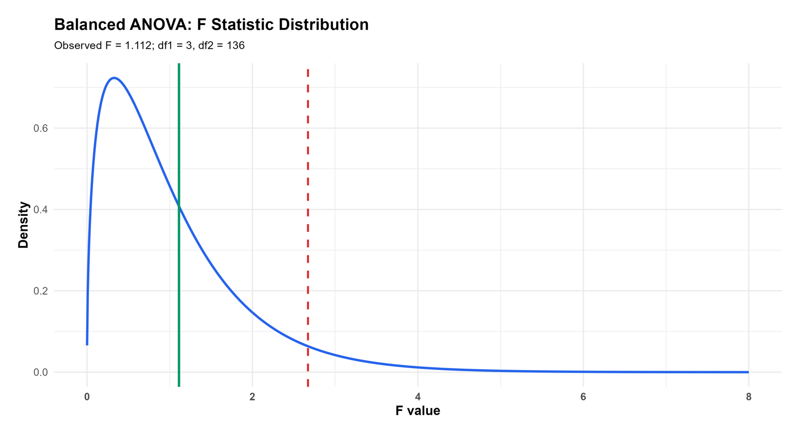
The R F distribution curve confirms the same decision as Python. The observed F statistic is 1.11, and the critical F value is 2.67.
The observed F statistic remains to the left of the critical F line. This confirms that the balanced ANOVA result is not statistically significant at the .05 level.
In reporting, this chart verifies that the non-significant decision is stable across software. Both Python and R show that the balanced group means do not differ enough to reject the null hypothesis.
R Chart 6: Balanced ANOVA Residual Histogram
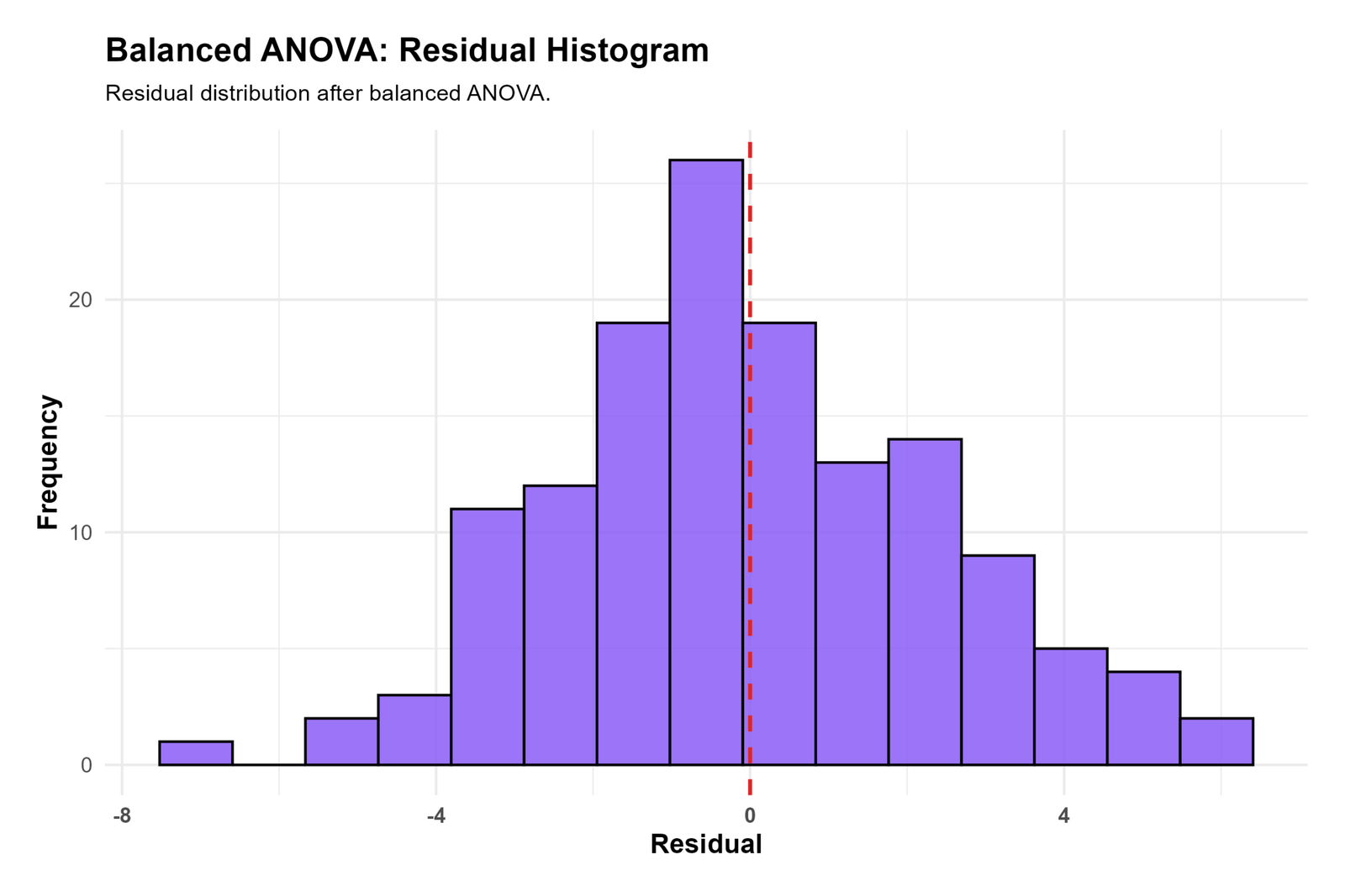
The R residual histogram confirms that residuals are centered near zero. This means the balanced group means are located near the center of the observed scores for many cases.
The distribution still has values on both sides of zero, showing that the model leaves considerable within-group variation. This matches the large within-group sum of squares.
In reporting, this chart supports the same diagnostic statement as the Python histogram. The balanced ANOVA residuals are centered around zero, but the model does not explain most of the individual score variation.
R Chart 7: Balanced ANOVA Effect Size Summary
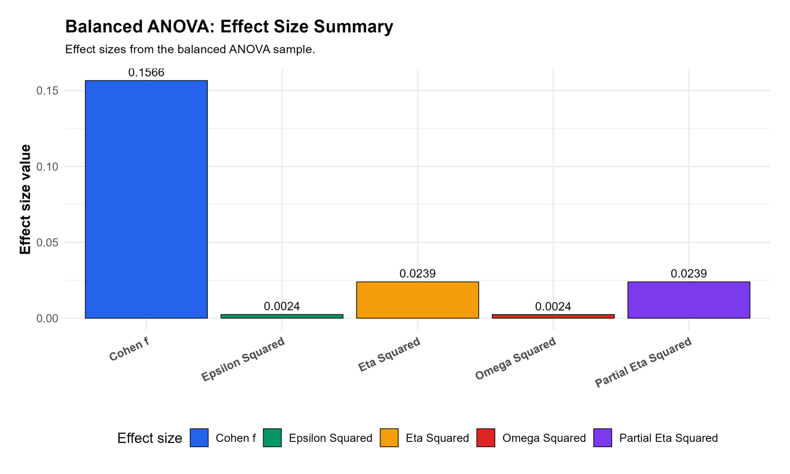
This R chart confirms the same effect-size values. Cohen’s f is 0.1566, eta squared and partial eta squared are 0.0239, and omega squared and epsilon squared are 0.0024.
The chart makes the practical result clear. The balanced studytime effect is small, and the adjusted effect-size measures are close to zero. This means the balanced sample does not support a strong practical group effect.
In the final article, this chart should be used as the practical interpretation summary. It confirms that the balanced ANOVA result is both statistically non-significant and small in explained variance.
SPSS Output Interpretation for Balanced ANOVA
The SPSS output PDF should be used as the final software verification file for the Balanced ANOVA workflow. It documents the balanced one-way ANOVA procedure, group comparison, equal-size sample structure, ANOVA table, assumption checks and reporting evidence.
Download Balanced ANOVA SPSS Output PDF
SPSS Output Items to Read
| SPSS Output Item | What It Shows | How It Is Used | Reporting Meaning |
|---|---|---|---|
| Case processing or group count output | Balanced group sizes. | Confirms that each studytime group contributes the same number of cases. | Report that the balanced ANOVA used 35 cases per group. |
| Descriptives | Mean, standard deviation and confidence interval for each balanced group. | Shows the direction of the group mean pattern. | Report means before the F test. |
| Homogeneity test | Levene-style equal variance evidence. | Checks whether ordinary ANOVA variance assumption is reasonable. | Report before final ANOVA interpretation. |
| ANOVA table | Between-groups and within-groups variation, F statistic and significance. | Tests whether balanced group means differ. | Report F, df and p value. |
| Effect size | Eta squared or partial eta squared. | Shows practical size of the balanced group effect. | Report explained variance and interpretation. |
| Residual diagnostics | Residual distribution and outlier behavior. | Checks model assumptions. | Discuss residual shape and any diagnostic caution. |
SPSS Reporting Summary
The SPSS interpretation should state that the balanced ANOVA used equal group sizes across the four studytime categories. The balanced group means were close together, and the ANOVA did not show a statistically significant group effect. The effect-size values were small, so the balanced result should be reported as a weak group effect in this equal-size sample.
The SPSS output PDF should be placed in the downloads section and referenced in the SPSS interpretation section. This gives readers a direct verification file for the balanced ANOVA result.
SPSS, R, Python and Excel Workflows for Balanced ANOVA
The same Balanced ANOVA workflow can be reproduced in SPSS, R, Python and Excel. The important step is not only running ANOVA. The important step is first creating or selecting a balanced sample where every group has the same number of observations.
SPSS Workflow
| Step | SPSS Menu or Syntax | Purpose |
|---|---|---|
| Open data | File > Open > Data | Load the dataset with G3 and studytime. |
| Create balanced sample | Data > Select Cases or sampling syntax | Keep the same number of cases in each studytime group. |
| Check group counts | Analyze > Descriptive Statistics > Frequencies | Confirm 35 cases per group. |
| Run one-way ANOVA | Analyze > Compare Means > One-Way ANOVA | Compare balanced group means. |
| Request homogeneity | Options > Homogeneity of variance test | Check equal variance assumption. |
| Export output | OUTPUT EXPORT | Save the SPSS PDF for reporting. |
R Workflow
| Step | R Action | Purpose |
|---|---|---|
| Read data | read.csv("dataset.csv") | Load the dataset. |
| Set factor | as.factor(studytime) | Define studytime as a categorical group. |
| Balance groups | dplyr::slice_sample(n = 35) | Select equal cases from each group. |
| Check counts | table(balanced$studytime) | Verify equal group sizes. |
| Run ANOVA | aov(G3 ~ studytime, data = balanced) | Fit the balanced ANOVA. |
| Effect size | Manual formulas or effectsize | Calculate eta squared, omega squared and Cohen’s f. |
Python Workflow
| Step | Python Action | Purpose |
|---|---|---|
| Read data | pandas.read_csv() | Load dataset. |
| Convert variables | pd.to_numeric() and category conversion | Prepare G3 and studytime. |
| Balance sample | groupby().sample(n=35) | Select equal observations from each studytime group. |
| Run model | ols("G3 ~ C(studytime)", data=balanced).fit() | Fit balanced ANOVA. |
| ANOVA table | sm.stats.anova_lm() | Extract F statistic and p value. |
| Effect size | Sum-of-squares formulas | Calculate practical magnitude. |
Excel Workflow
| Excel Task | Tool or Formula | Purpose |
|---|---|---|
| Sort by group | Sort or filter studytime | Separate the four groups. |
| Create equal groups | Select the same number of rows per group | Build balanced columns or a balanced sheet. |
| Check counts | =COUNT(group_range) | Confirm equal group sizes. |
| Run ANOVA | Data Analysis ToolPak > ANOVA: Single Factor | Get ANOVA table. |
| Calculate eta squared | =SS_Between/SS_Total | Calculate effect size. |
| Create charts | Insert > Chart | Show group means, residuals and effect size. |
Code Blocks for Balanced ANOVA
SPSS Syntax for Balanced ANOVA
* Balanced ANOVA in SPSS.
* Dependent variable: G3.
* Grouping factor: studytime.
* Use a balanced sample with equal group sizes before running ANOVA.

TITLE "Balanced ANOVA: G3 by Studytime".

FREQUENCIES VARIABLES=studytime.

ONEWAY G3 BY studytime
  /STATISTICS DESCRIPTIVES HOMOGENEITY
  /MISSING ANALYSIS.

UNIANOVA G3 BY studytime
  /METHOD=SSTYPE(3)
  /INTERCEPT=INCLUDE
  /PRINT=DESCRIPTIVE ETASQ HOMOGENEITY
  /SAVE=PRED RESID
  /CRITERIA=ALPHA(.05)
  /DESIGN=studytime.

EXAMINE VARIABLES=RES_1
  /PLOT HISTOGRAM NPPLOT BOXPLOT
  /STATISTICS DESCRIPTIVES
  /CINTERVAL 95
  /MISSING LISTWISE
  /NOTOTAL.

OUTPUT EXPORT
  /CONTENTS EXPORT=VISIBLE
  /PDF DOCUMENTFILE="Balanced-ANOVA-SPSS-Output.pdf".
Python Code for Balanced ANOVA
import pandas as pd
import numpy as np
import statsmodels.api as sm
from statsmodels.formula.api import ols
import scipy.stats as stats

df = pd.read_csv("dataset.csv")

df["G3"] = pd.to_numeric(df["G3"], errors="coerce")
df["studytime"] = df["studytime"].astype("category")

df_model = df.dropna(subset=["G3", "studytime"]).copy()

# Balance to the smallest group size
min_n = df_model.groupby("studytime").size().min()

balanced = (
    df_model
    .groupby("studytime", group_keys=False)
    .sample(n=min_n, random_state=123)
    .copy()
)

print("Original group sizes")
print(df_model["studytime"].value_counts().sort_index())

print("Balanced group sizes")
print(balanced["studytime"].value_counts().sort_index())

# Balanced one-way ANOVA
model = ols("G3 ~ C(studytime)", data=balanced).fit()
anova_table = sm.stats.anova_lm(model, typ=2)
print(anova_table)

# Group means
group_summary = balanced.groupby("studytime")["G3"].agg(["count", "mean", "std", "var"])
print(group_summary)

# Effect sizes
ss_between = anova_table.loc["C(studytime)", "sum_sq"]
df_between = anova_table.loc["C(studytime)", "df"]
ss_within = anova_table.loc["Residual", "sum_sq"]
df_within = anova_table.loc["Residual", "df"]
ss_total = ss_between + ss_within
ms_within = ss_within / df_within

eta_squared = ss_between / ss_total
partial_eta_squared = ss_between / (ss_between + ss_within)
omega_squared = (ss_between - df_between * ms_within) / (ss_total + ms_within)
epsilon_squared = (ss_between - df_between * ms_within) / ss_total
cohen_f = np.sqrt(eta_squared / (1 - eta_squared))

print("Eta squared:", eta_squared)
print("Partial eta squared:", partial_eta_squared)
print("Omega squared:", omega_squared)
print("Epsilon squared:", epsilon_squared)
print("Cohen's f:", cohen_f)

# Residuals
balanced["fitted"] = model.fittedvalues
balanced["residual"] = model.resid

# Assumption support
groups = [
    group["G3"].dropna().values
    for name, group in balanced.groupby("studytime")
]

levene_stat, levene_p = stats.levene(*groups, center="median")
print("Levene statistic:", levene_stat)
print("Levene p:", levene_p)
R Code for Balanced ANOVA
library(dplyr)

df <- read.csv("dataset.csv")

df$G3 <- as.numeric(df$G3)
df$studytime <- as.factor(df$studytime)

df_model <- na.omit(df[, c("G3", "studytime")])

# Original group sizes
table(df_model$studytime)

# Balance to smallest group size
min_n <- min(table(df_model$studytime))

set.seed(123)
balanced <- df_model %>%
  group_by(studytime) %>%
  slice_sample(n = min_n) %>%
  ungroup()

# Balanced group sizes
table(balanced$studytime)

# Balanced group means
aggregate(G3 ~ studytime, data = balanced, FUN = function(x) {
  c(n = length(x), mean = mean(x), sd = sd(x), variance = var(x))
})

# Balanced ANOVA model
model <- aov(G3 ~ studytime, data = balanced)
summary(model)

# Effect size calculation
anova_table <- summary(model)[[1]]

ss_between <- anova_table["studytime", "Sum Sq"]
df_between <- anova_table["studytime", "Df"]
ss_within <- anova_table["Residuals", "Sum Sq"]
df_within <- anova_table["Residuals", "Df"]
ss_total <- ss_between + ss_within
ms_within <- ss_within / df_within

eta_squared <- ss_between / ss_total
partial_eta_squared <- ss_between / (ss_between + ss_within)
omega_squared <- (ss_between - df_between * ms_within) / (ss_total + ms_within)
epsilon_squared <- (ss_between - df_between * ms_within) / ss_total
cohen_f <- sqrt(eta_squared / (1 - eta_squared))

data.frame(
  eta_squared = eta_squared,
  partial_eta_squared = partial_eta_squared,
  omega_squared = omega_squared,
  epsilon_squared = epsilon_squared,
  cohen_f = cohen_f
)

# Residual diagnostics
par(mfrow = c(2, 2))
plot(model)
Excel Formulas for Balanced ANOVA
Step 1:
Separate data by studytime group.

Step 2:
Use the same number of rows from each group.

Balanced group count:
=COUNT(group_range)

Group mean:
=AVERAGE(group_range)

Group standard deviation:
=STDEV.S(group_range)

Run balanced ANOVA:
Data > Data Analysis > ANOVA: Single Factor

Total sum of squares:
=SS_Between + SS_Within

Mean square between:
=SS_Between / df_Between

Mean square within:
=SS_Within / df_Within

F statistic:
=MS_Between / MS_Within

Eta squared:
=SS_Between / SS_Total

Omega squared:
=(SS_Between - df_Between * MS_Within) / (SS_Total + MS_Within)

Cohen's f:
=SQRT(EtaSquared / (1 - EtaSquared))

Residual:
=Observed_G3 - Group_Mean
APA Reporting Wording
When reporting Balanced ANOVA, clearly say that the analysis used an equal-size sample. This is important because the result is not the same as a full unbalanced ANOVA result. Report the balanced group size, group means, F statistic, degrees of freedom, p value and effect size.
APA-style report: A balanced one-way ANOVA was conducted to compare G3 final grade across four studytime groups after equalizing the sample to 35 cases per group. The balanced group means were 12.229, 13.143, 12.886 and 13.057. The observed F statistic was 1.11, which was below the critical F value of 2.67; therefore, the balanced ANOVA did not show a statistically significant difference among studytime groups at α = .05. The effect size was small, η² = .0239, with Cohen’s f = .1566.
Short reporting version: The balanced ANOVA used 35 cases per studytime group and did not find a significant group effect, F ≈ 1.11, η² = .0239, Cohen’s f = .1566.
Common Mistakes
| Mistake | Why It Is Wrong | Correct Practice |
|---|---|---|
| Calling the full dataset balanced | The original group sizes are unequal. | Check group counts before using the word balanced. |
| Not explaining how balancing was done | Readers need to know whether cases were sampled, weighted or removed. | State that 35 cases per group were used. |
| Comparing balanced and unbalanced results as identical | They answer different sample questions. | Report balanced ANOVA as an equal-size sensitivity analysis. |
| Ignoring reduced power | Balancing by subsampling removes many observations from larger groups. | Mention the trade-off between equal group size and lower total N. |
| Reporting only the F statistic | The F statistic does not show practical magnitude. | Report eta squared, omega squared and Cohen’s f. |
| Skipping assumptions | Balanced ANOVA still requires diagnostic review. | Check ANOVA Assumptions, Levene Test, residual histogram and outliers. |
When to Use Balanced ANOVA
Use Balanced ANOVA when each group has the same sample size or when the research design intentionally requires equal group representation. It is common in controlled experiments, classroom examples, simulation studies and sensitivity checks where unequal group sizes may affect interpretation.
| Situation | Balanced ANOVA Use | Reporting Caution |
|---|---|---|
| Experimental design | Each treatment group has equal N. | Report equal group sizes and ANOVA result. |
| Unbalanced observational data | Use balanced subsample as sensitivity check. | Do not hide the original unequal group sizes. |
| Teaching ANOVA | Equal groups make formulas easier to explain. | Clarify that real data may be unbalanced. |
| Comparing software outputs | Equal groups simplify SPSS, R, Python and Excel comparison. | Use the same balanced sample in all software. |
| Large group imbalance | Balancing prevents larger groups from dominating. | Report that smaller N may reduce power. |
For related mean-comparison tutorials, see ANOVA in SPSS, ANOVA in Python, ANOVA in R, ANOVA Effect Size, ANOVA Assumptions, ANCOVA, T Test vs ANOVA, Two Sample T Test, and Welch’s T Test.
Downloads and Resources for Balanced ANOVA
Use these resources to reproduce the Balanced ANOVA workflow. The SPSS PDF verifies the balanced ANOVA output, while the script and workbook placeholders can be replaced after uploading final files to the WordPress Media Library.
Download Dataset
Practice dataset with G3 and studytime variables.
Download Balanced ANOVA SPSS Output PDF
SPSS output PDF for balanced ANOVA verification and reporting.
Download Python Script
Python code for balancing groups, running ANOVA, creating charts and calculating effect size.
Download R Script and Excel Workbook
R validation workflow and Excel formulas for balanced ANOVA.
FAQs About Balanced ANOVA
What is Balanced ANOVA?
Balanced ANOVA is an ANOVA design where every group has the same sample size. In this example, each studytime group contributes 35 cases.
What is the difference between balanced and unbalanced ANOVA?
Balanced ANOVA has equal group sizes, while unbalanced ANOVA has unequal group sizes. The original data were unbalanced, but the balanced sample used 35 cases per group.
Why use a balanced ANOVA?
Balanced ANOVA gives each group equal representation. It is useful for clean comparisons, teaching examples, controlled designs and sensitivity checks.
What was the balanced sample size in this example?
The balanced sample used 35 cases from each of the four studytime groups, giving a total balanced sample size of 140.
Was the balanced ANOVA significant?
No. The observed F statistic was 1.11 and the critical F value was 2.67, so the balanced ANOVA did not reject the null hypothesis at the .05 level.
What were the balanced group means?
The balanced group means were 12.229, 13.143, 12.886 and 13.057 for studytime groups 1, 2, 3 and 4.
What was the effect size for the balanced ANOVA?
Eta squared was .0239, partial eta squared was .0239, omega squared was .0024, epsilon squared was .0024 and Cohen’s f was .1566.
Does balancing always improve ANOVA?
No. Balancing can make group comparison cleaner, but if it is done by subsampling, it also reduces the total sample size and may reduce statistical power.
Should I report original group sizes in Balanced ANOVA?
Yes. Report both original group sizes and balanced group sizes so readers understand how the balanced sample was created.
How do I report Balanced ANOVA in APA format?
A concise report is: A balanced one-way ANOVA using 35 cases per studytime group did not show a significant group effect, F ≈ 1.11, η² = .0239, Cohen’s f = .1566.

