
Normality, Homogeneity of Variance, Independence, Residual Diagnostics and Outlier Review
ANOVA Assumptions: Normality, Homogeneity, Independence, Outliers, SPSS, Python, R and Excel Guide
ANOVA Assumptions are the diagnostic conditions that should be checked before interpreting an ANOVA F test. In this guide, G3 final grade is compared across studytime groups, and the assumption workflow checks group means, boxplots, residual histogram, residual Q-Q plot, residuals versus fitted values, Levene homogeneity test and outlier counts. The article explains one way ANOVA assumptions, assumptions of ANOVA, how to check ANOVA assumptions, Python charts, R validation charts, SPSS output, Excel workflow, APA reporting and related guides.
Quick Answer: ANOVA Assumptions Result
The worked ANOVA Assumptions example compares G3 final grade across four studytime groups. The group means rise from about 10.844 in studytime group 1 to 12.092 in group 2, 13.227 in group 3 and 13.057 in group 4. This gives a clear descriptive group pattern before the formal ANOVA result is interpreted.
The residual and assumption charts show a mostly usable ANOVA model, but not a perfect one. The Levene homogeneity check gives p = 0.3804, so the equal-variance assumption is supported. The residual histogram and Q-Q plot show residuals centered near zero, but the lower tail contains several large negative residuals. The outlier count chart shows 10 IQR outliers in studytime group 1, 8 in group 2, and 0 in groups 3 and 4.
Final interpretation: The ANOVA assumption checks support the use of ordinary ANOVA for the equal-variance condition because Levene’s test is not significant. The main caution is residual tail behavior and low-score outliers in studytime groups 1 and 2. These outliers should be reported as diagnostic review points, not deleted automatically.
Important reporting point: Do not write only “ANOVA assumptions were met.” A proper report should say that Levene’s test supported homogeneity of variance, residual plots were centered but showed lower-tail departures, and IQR outliers were found mainly in studytime groups 1 and 2.
Table of Contents
- What Are ANOVA Assumptions?
- ANOVA Assumptions Formula
- Diagnostic Null and Alternative Hypothesis
- Dataset and ANOVA Variables Used
- Python Chart-by-Chart Interpretation
- R Chart-by-Chart Validation
- SPSS Output Interpretation
- SPSS, R, Python and Excel Workflows
- Code Blocks for ANOVA Assumptions
- APA Reporting Wording
- Common Mistakes
- When to Check ANOVA Assumptions
- Downloads and Resources
- Related Guides
- FAQs
What Are ANOVA Assumptions?
ANOVA assumptions are the conditions that make the ANOVA F test trustworthy. The main assumptions are independent observations, a numeric dependent variable, approximately normal residuals, reasonably equal group variances and no extreme outlier problem that dominates the group comparison.
These assumptions should be checked before reporting the F test. ANOVA does not require every raw group distribution to be perfectly normal, especially in larger samples, but the residuals should be roughly centered and not dominated by extreme tail behavior. Group variances should also be similar enough that the within-group error term is fair across all groups.
In this example, studytime group means increase from group 1 to group 3 and remain high in group 4. That group pattern is meaningful, but the assumption checks decide how confidently the F test can be interpreted. The Levene chart supports homogeneity of variance, while residual and outlier plots show that the low-score tail needs to be acknowledged.
Simple definition: ANOVA assumptions are the diagnostic checks that show whether a group mean comparison can be trusted. They include independence, residual normality, equal variances and outlier review.
ANOVA assumption checking is closely related to Normal Distribution, Shapiro-Wilk Test, Skewness and Kurtosis Normality Check, Q-Q Plot Normality Check, P-P Plot Normality Check, Levene Test, Brown-Forsythe Test, Bartlett’s Test, and Outlier Detection.
ANOVA Assumptions Formula
A one-way ANOVA model can be written as:
Here, Yij is the observed outcome for case j in group i, μ is the grand mean, τi is the group effect, and εij is the residual error. The assumption checks mostly focus on the behavior of εij, not only on the raw outcome.
Residual Normality Assumption
The residuals should be approximately centered around zero and should not show extreme nonnormality. In the supplied residual plots, the center is acceptable, but the lower tail has several large negative residuals. That means the report should say that residual normality is reasonable in the center but has lower-tail departures.
Equal Variance Assumption
The groups should have similar variance. The Levene chart reports p = 0.3804, which is greater than .05. This supports the homogeneity of variance assumption for the studytime group comparison.
ANOVA F Statistic
The F statistic compares between-group mean variation with within-group variation. If residuals and variances behave reasonably, this ratio provides the test of whether group means differ more than expected by random within-group error.
| Assumption | Meaning | Evidence in This Output | Reporting Meaning |
|---|---|---|---|
| Independent observations | Each student record should be separate. | Checked from study design, not from a chart. | State that independence was assumed from the sampling structure. |
| Numeric dependent variable | The outcome should be scale-level. | G3 is a numeric final grade. | ANOVA is suitable for comparing group means of G3. |
| Residual normality | Model errors should be approximately normal. | Center is acceptable, lower tail departs. | Report residual tail caution. |
| Homogeneity of variance | Group variances should be similar. | Levene p = 0.3804. | Equal variance assumption is supported. |
| Outlier review | Extreme values should not dominate the result. | 10 outliers in group 1, 8 in group 2. | Outliers should be reviewed and disclosed. |
Diagnostic Null and Alternative Hypothesis for ANOVA Assumptions
The main ANOVA hypothesis tests group means. Assumption tests answer a different question: whether the diagnostic conditions are reasonable enough to interpret the F test.
| Diagnostic Check | Null Hypothesis or Diagnostic Rule | Result in This Output | Decision |
|---|---|---|---|
| Levene homogeneity test | Group variances are equal. | p = 0.3804. | Do not reject equal variances. |
| Residual histogram | Residuals should be centered and roughly symmetric. | Centered near zero with lower-tail cases. | Acceptable center, tail caution. |
| Residual Q-Q plot | Residuals should follow the diagonal line. | Central points follow line; lower tail departs. | Normality mostly acceptable but not perfect. |
| Residuals vs fitted | Residuals should not show a curve or funnel. | Vertical group bands with no strong funnel. | No major variance pattern, but outliers exist. |
| IQR outlier count | No group should be dominated by extreme values. | Group 1 = 10, group 2 = 8, group 3 = 0, group 4 = 0. | Outliers are concentrated in lower studytime groups. |
Decision for this example: The homogeneity of variance assumption is supported by Levene’s test, but residual tail behavior and low-score outliers should be reported. The ordinary ANOVA can be interpreted with this diagnostic caution rather than claiming that every assumption is perfect.
Dataset and ANOVA Variables Used
The worked example uses a student performance dataset. The dependent variable is G3 final grade, and the grouping factor is studytime. The analysis compares mean G3 across four studytime groups and then checks whether the assumptions behind the ANOVA comparison are reasonable.
| Variable | Role | Why It Matters for ANOVA Assumptions | Where It Appears in Output |
|---|---|---|---|
| G3 | Dependent variable | Final grade outcome being compared across groups. | Means, boxplots, residuals and outlier checks. |
| studytime | Grouping factor | Defines the four groups in the one-way ANOVA. | Group mean charts, boxplots and outlier counts. |
| Residuals | Model errors | Used to check normality and model fit. | Histogram, Q-Q plot and residuals vs fitted plot. |
| Group variance | Homogeneity condition | Shows whether within-group spread is similar. | Levene homogeneity test and boxplot spread. |
| IQR outlier flags | Outlier review | Shows where unusual low or high values occur. | Outlier count by group chart. |
Assumption checking should be interpreted together with Descriptive Statistics, Mean Median and Mode, Standard Deviation, Variance, Interquartile Range, Five Number Summary, Histogram Interpretation, and Box Plot Interpretation.
Python Chart-by-Chart Interpretation
The Python charts below show the first ANOVA assumption workflow. They explain the studytime group means, group spread, residual shape, Q-Q plot behavior, residuals against fitted group means, Levene homogeneity test and IQR outlier count.
Python Chart 1: Group Means with 95% Confidence Intervals
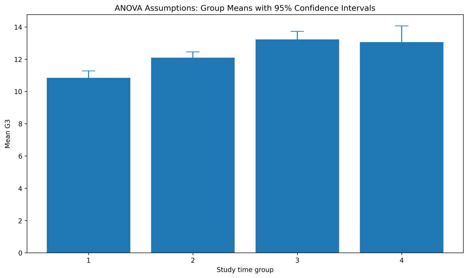
This chart shows the mean G3 score for each studytime group. The mean is lowest in group 1, increases in group 2, reaches its highest level in group 3 and remains high in group 4. The visible pattern is an upward movement in final grade as studytime category increases from 1 to 3.
The confidence intervals are relatively narrow for the first three groups and wider for group 4, which is expected when a group has fewer observations or more uncertainty. The chart supports the descriptive claim that the studytime groups do not have identical mean G3 values.
In the article report, this chart should introduce the ANOVA comparison. It shows the group mean pattern, but it does not by itself prove that ANOVA assumptions are satisfied. The assumption decision must be based on the residual charts, Levene test and outlier count that follow.
Python Chart 2: Boxplot of G3 by Study Time
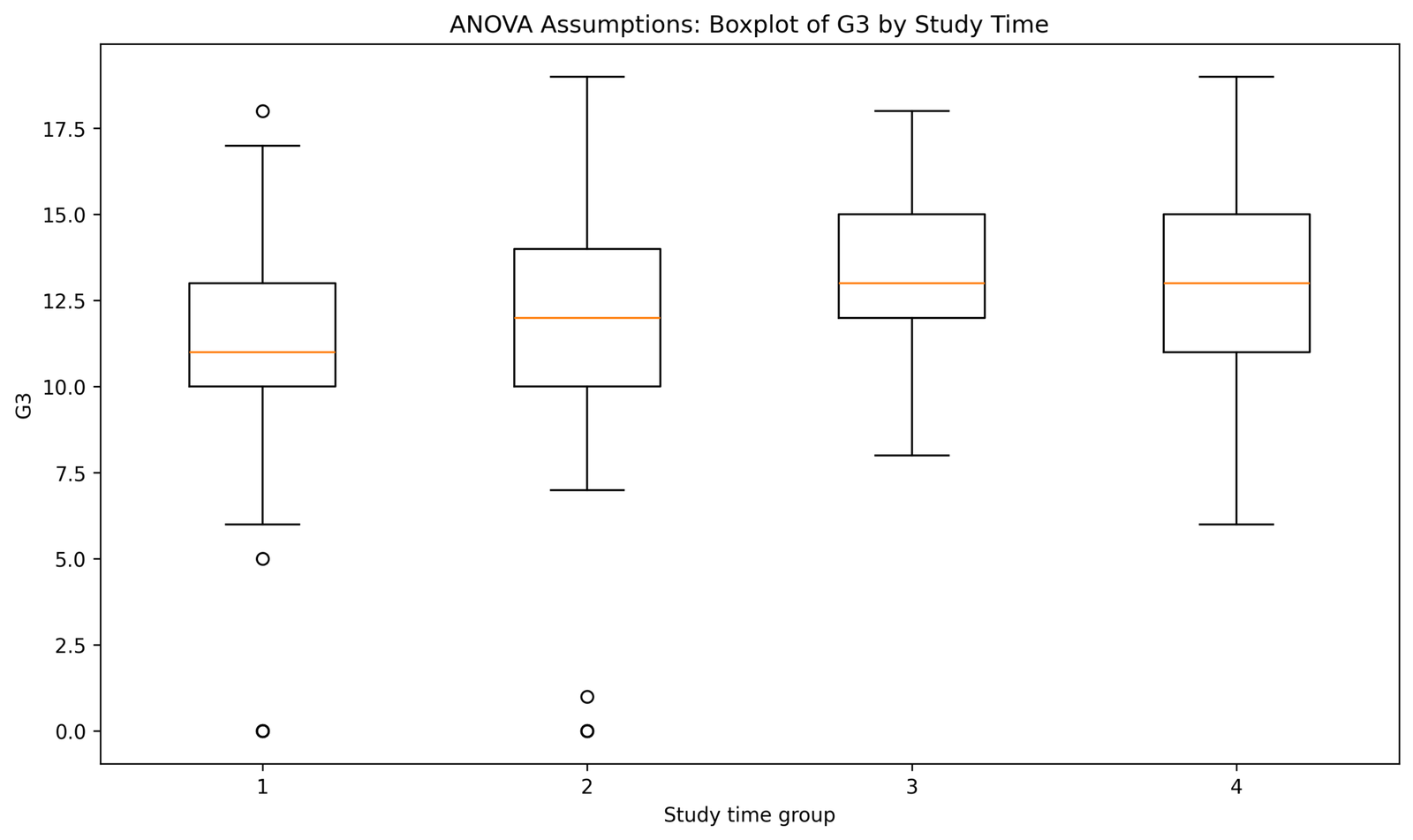
This boxplot shows the median, interquartile range, whiskers and possible outliers for G3 in each studytime group. Group 1 has the lowest center, group 2 is higher, and groups 3 and 4 have higher medians. This matches the group mean pattern from the previous chart.
The low outliers are mainly visible in groups 1 and 2. Group 1 includes values near 0 and around 5, and group 2 also includes very low points. Groups 3 and 4 do not show the same low-outlier pattern in this output.
In reporting, this chart supports two statements: the group centers differ, and the outlier problem is concentrated in the lower studytime groups. These outliers should be reviewed through Outlier Detection, Z Score, Interquartile Range and Studentized Residuals rather than removed automatically.
Python Chart 3: Residual Histogram
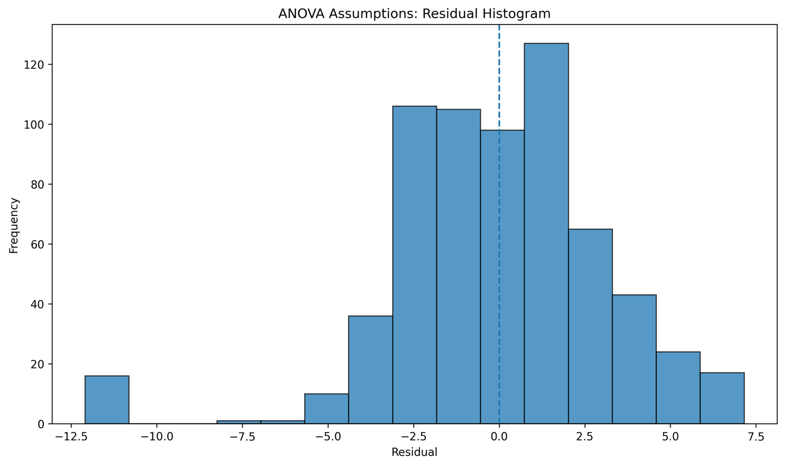
This histogram shows the residual distribution from the ANOVA model. Most residuals are concentrated around zero, with the tallest bars around the center and slightly positive residual region. This means the fitted group means capture the main center of the data reasonably well.
The lower tail extends much farther than the upper tail, with residuals reaching near -12.5. The right side extends only to about 7.5. This tells us that several observed G3 values were much lower than their fitted group mean, which is consistent with the low outliers seen in groups 1 and 2.
In reporting, this chart should be described as mostly centered but left-tailed. It supports a cautious normality statement: residuals are not randomly extreme throughout the whole dataset, but the lower-tail cases should be acknowledged before interpreting the ANOVA result.
Python Chart 4: Residual Q-Q Plot
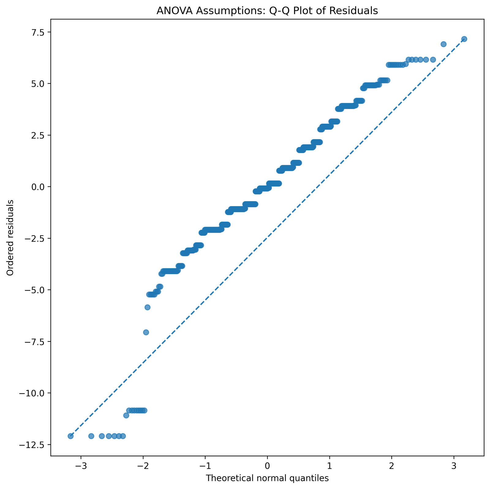
The Q-Q plot shows that the central residuals follow the diagonal trend fairly well. This means the middle of the residual distribution is reasonably close to normal.
The strongest departure occurs in the lower-left tail. Several residuals fall far below the diagonal line, showing unusually low observed G3 values compared with their fitted group means. The upper tail also departs from the line, but the lower-tail departure is the clearer diagnostic issue.
In reporting, this chart should not be described as perfect normality. A better statement is that residual normality is acceptable in the center but shows tail departures caused by extreme low residuals. Formal normality tools such as Shapiro-Wilk Test, Anderson-Darling Test, Jarque-Bera Test, Lilliefors Test and Kolmogorov-Smirnov Test can be added if a formal test is needed.
Python Chart 5: Residuals vs Fitted Values
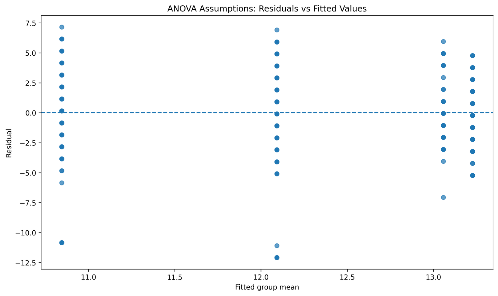
This chart plots residuals against the fitted group means. The points appear in vertical bands because fitted values are group means, not continuous predictions. Most residuals are distributed around the zero line, which means many observations are reasonably close to their group mean.
The main issue is the set of large negative residuals, especially below -10 in the fitted-value regions near groups 1 and 2. These cases match the low outliers shown in the boxplot and the long left tail shown in the histogram. There is no strong funnel shape across fitted values, so the plot does not show a severe variance pattern.
In reporting, this chart supports the statement that residuals were mostly centered around zero, with several unusually low cases. The absence of a clear funnel agrees with the Levene result, while the extreme negative residuals support the need for outlier review.
Python Chart 6: Levene Homogeneity Test
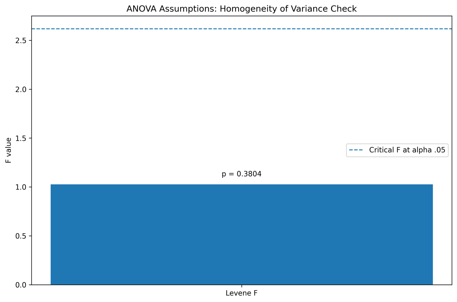
This chart shows the Levene homogeneity test result. The Levene F statistic is around 1.0 and the p value displayed on the chart is 0.3804. The critical F line is much higher than the observed Levene statistic.
Because the p value is greater than .05, the equal-variance assumption is supported. This means the studytime groups do not show statistically significant variance differences in this assumption check.
In reporting, write that Levene’s test was not significant, p = .380, so the homogeneity of variance assumption was acceptable. This result supports ordinary ANOVA rather than immediately requiring Welch ANOVA or Brown-Forsythe correction.
Python Chart 7: IQR Outlier Count by Group
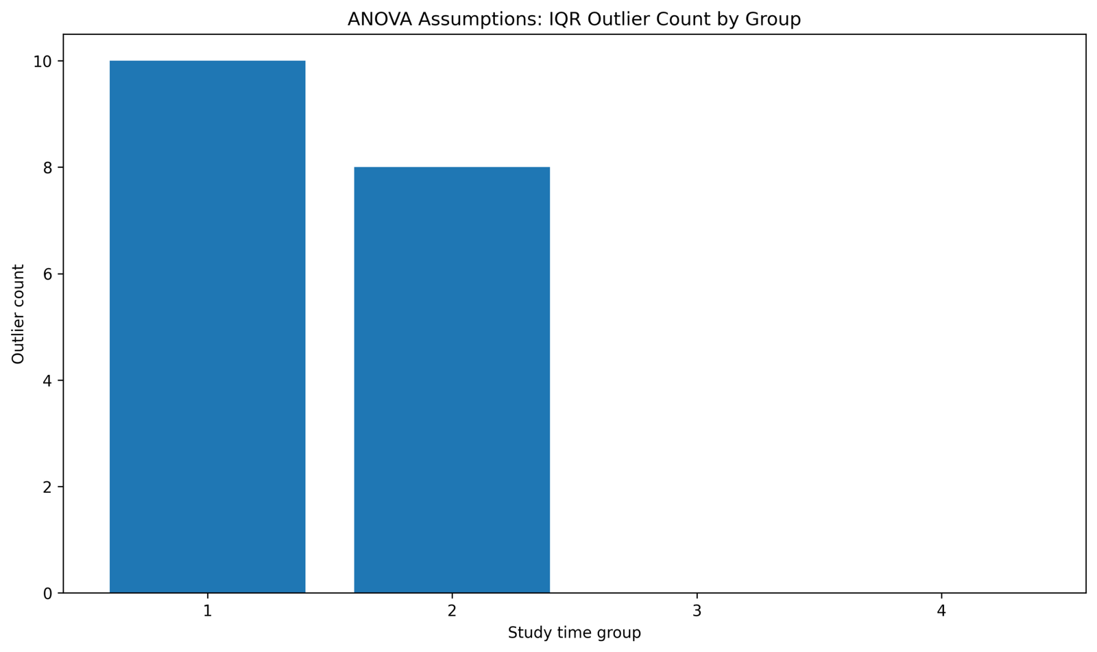
This chart counts possible IQR outliers in each studytime group. Studytime group 1 has 10 outliers, group 2 has 8, and groups 3 and 4 have 0 outliers.
The result shows that the outlier issue is not evenly distributed across groups. It is concentrated in the lower studytime groups, which is consistent with the boxplot and residual charts showing unusually low G3 values.
In reporting, this chart should be used to say that the ANOVA included outlier review and that outliers were mainly found in groups 1 and 2. The correct conclusion is review and sensitivity checking, not automatic deletion.
R Chart-by-Chart Validation
The R validation charts confirm the same ANOVA assumption pattern in a second workflow. The values and visual shapes match the Python interpretation: means increase across studytime groups, Levene’s test supports equal variances, and residual diagnostics show lower-tail departures from normality.
R Chart 1: Group Means with 95% Confidence Intervals
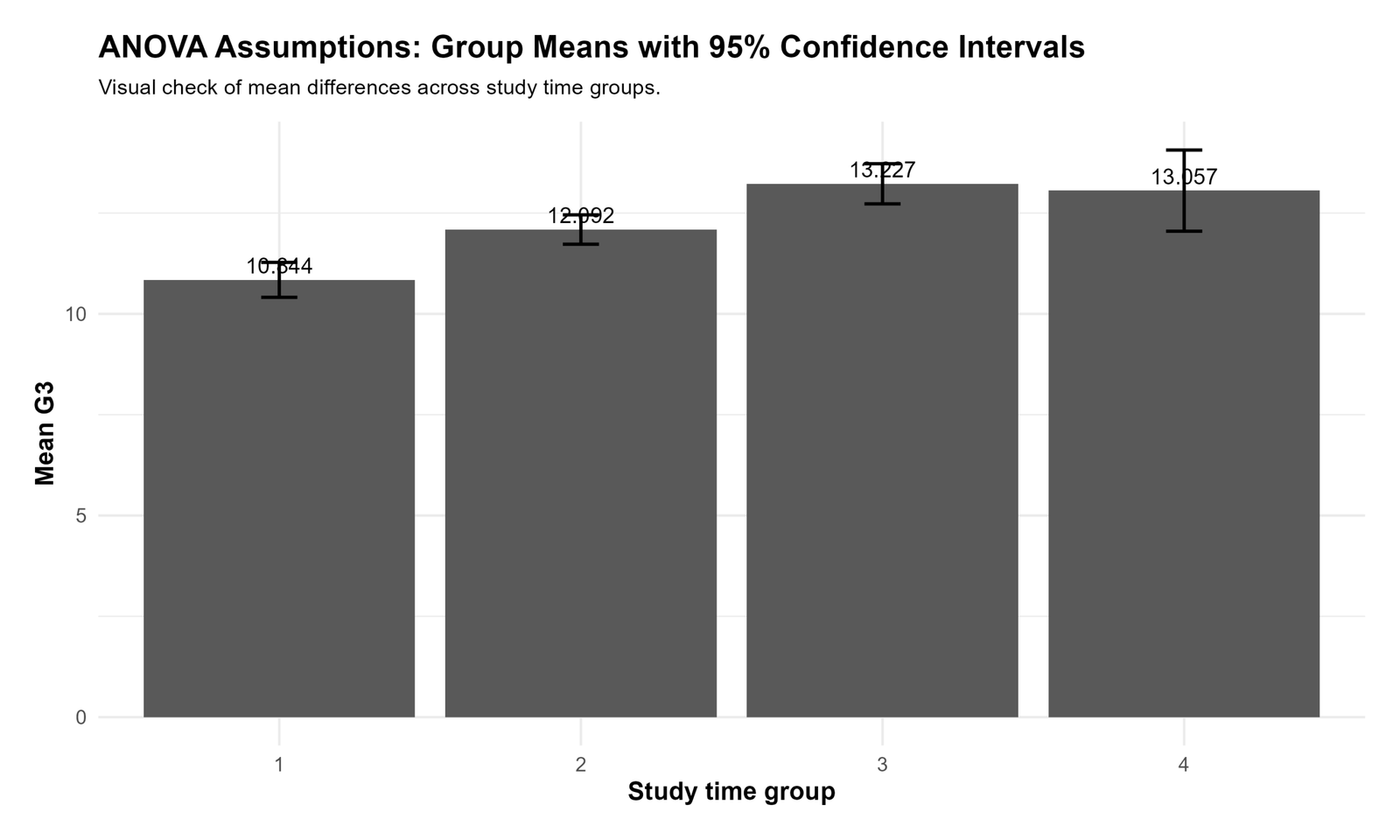
This R chart labels the group means directly. The mean G3 values are 10.844 for studytime group 1, 12.092 for group 2, 13.227 for group 3 and 13.057 for group 4.
The values confirm that the lowest performance is in group 1 and the highest performance is in group 3, with group 4 remaining close to group 3. This is the same pattern shown in the Python group-mean chart.
In reporting, this chart supports the descriptive group comparison before the assumption discussion. It is useful for explaining the direction of the group difference, while the later charts explain whether the ANOVA assumptions are acceptable.
R Chart 2: Boxplot of G3 by Study Time
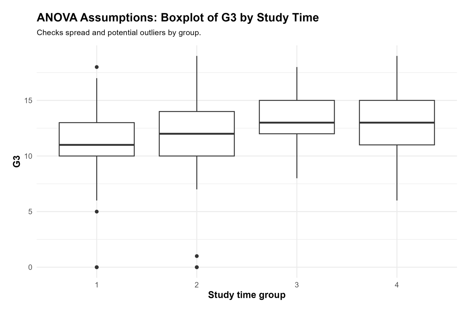
The R boxplot confirms that groups 3 and 4 have higher centers than groups 1 and 2. The group 1 and group 2 boxes sit lower, while groups 3 and 4 are centered closer to the higher G3 range.
Low outliers are visible in groups 1 and 2. Group 1 includes low values near 0 and 5, while group 2 includes very low observations near 0 and 1. Groups 3 and 4 do not show the same low-outlier pattern.
In reporting, this chart confirms that the outlier concern is concentrated in the lower studytime groups. If the final report includes a sensitivity check, it should focus on whether these low-score cases affect the ANOVA conclusion.
R Chart 3: Residual Histogram
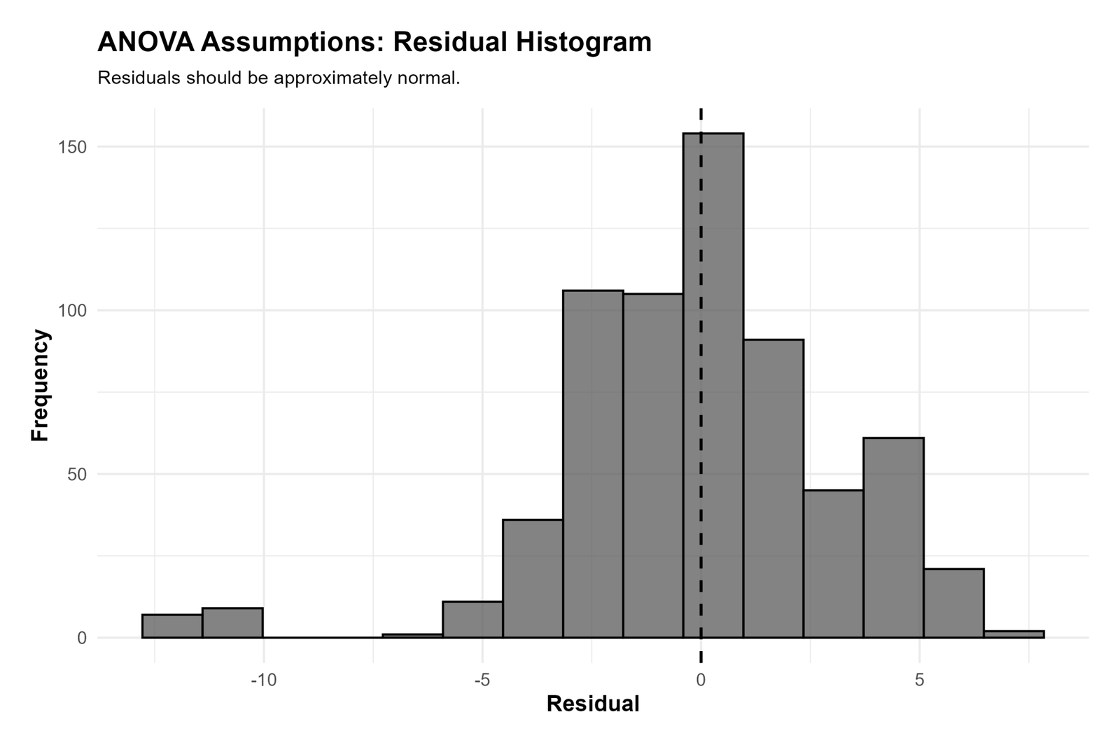
The R residual histogram is centered near zero and has its largest bars in the middle of the distribution. This confirms that the group means generally fit the center of the data.
The left side of the histogram extends farther than the right side, with several residuals below -10. This means some students scored far below the mean expected for their studytime group. The chart therefore confirms the same lower-tail issue shown in the Python residual histogram.
In reporting, say that the residual distribution was centered near zero but showed a heavier lower tail. This statement is more accurate than simply saying that the normality assumption was fully met.
R Chart 4: Residual Q-Q Plot
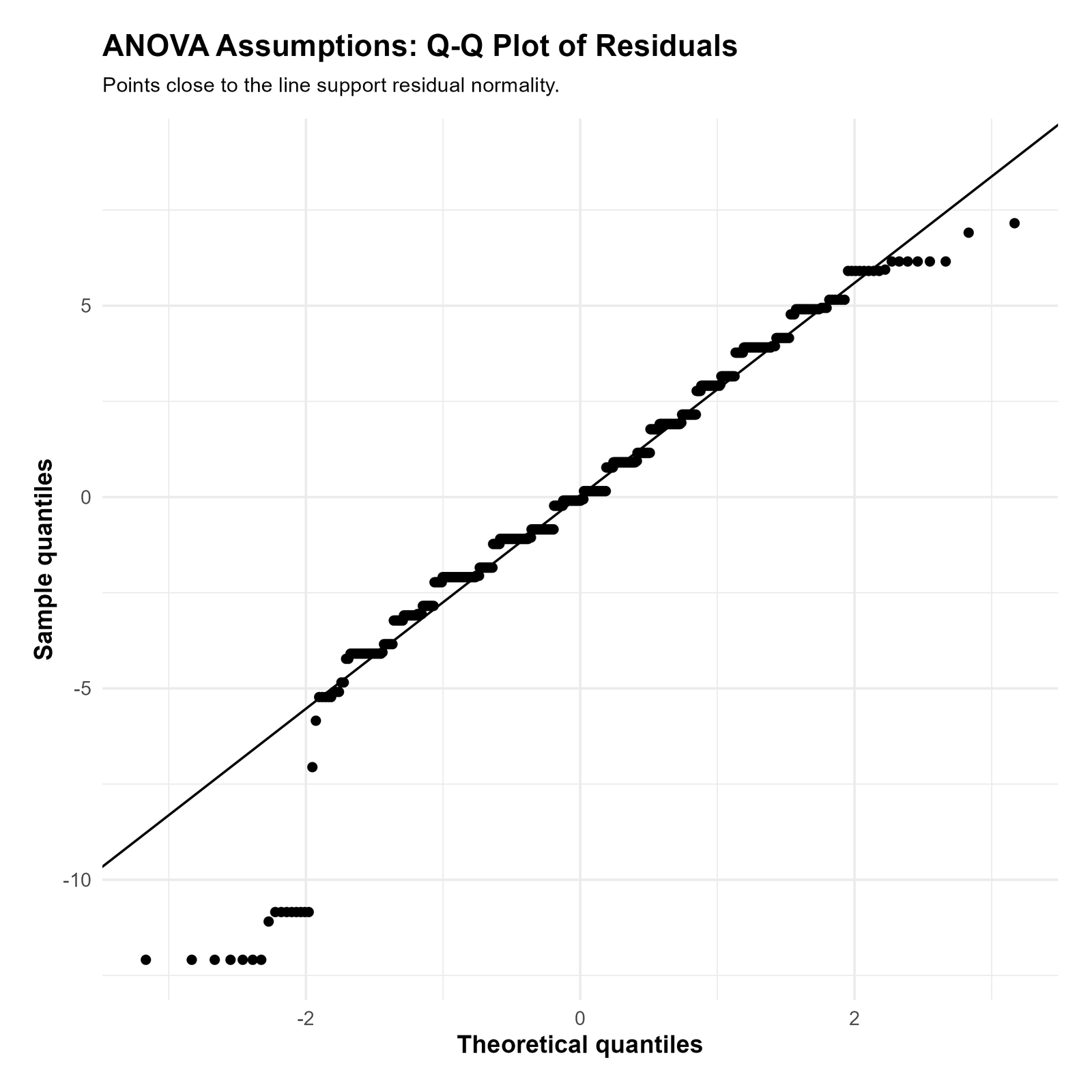
The R Q-Q plot shows that most central residuals lie close to the diagonal line. This supports approximate normality for the middle part of the residual distribution.
The lower-left tail departs strongly from the line, with several points far below the expected normal pattern. The upper-right tail also bends away from the line, but the lower-tail departure is the clearer diagnostic problem.
In reporting, this chart supports the same conclusion as the Python Q-Q plot: residual normality is reasonable in the center but has tail departures. This should be described as a caution, not ignored.
R Chart 5: Residuals vs Fitted Values
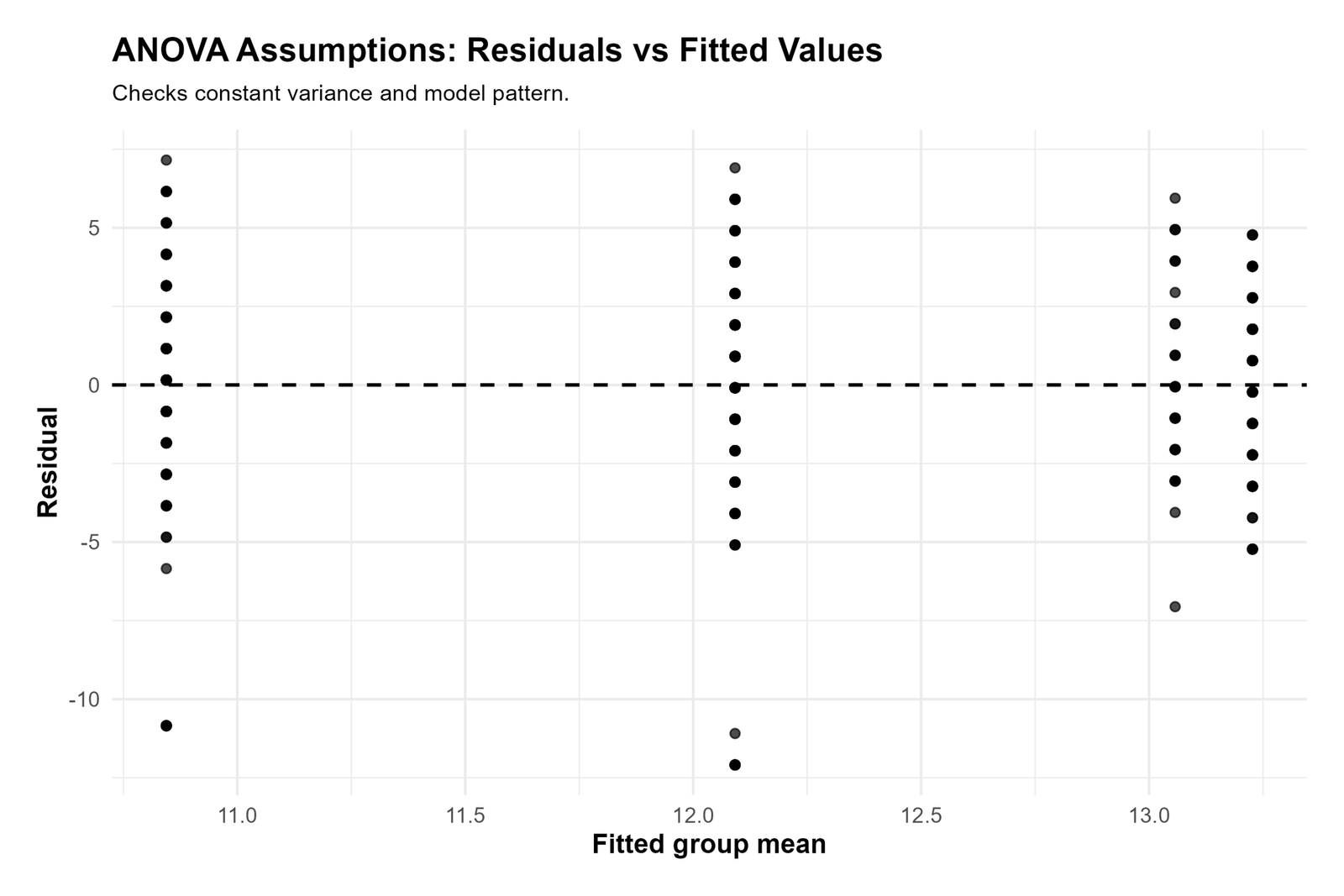
This plot shows residuals in vertical bands because the fitted values are group means. Most points are close to the zero residual line, which indicates that many observations are reasonably close to their group mean.
The visible large negative residuals confirm the same issue seen in the histogram, Q-Q plot and boxplot. They are not random small deviations; they are unusually low G3 values relative to their fitted group means.
In reporting, this plot supports two diagnostic statements: no strong funnel pattern is visible, and several extreme negative residuals should be reviewed. The absence of a strong funnel agrees with the Levene p value of .3804.
R Chart 6: Levene Homogeneity Test
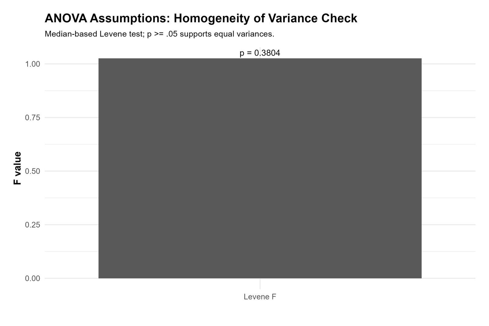
This R chart reports the same Levene homogeneity result as the Python output. The p value is 0.3804, which is above .05.
The result means that there is no statistically significant evidence that studytime group variances differ. The equal-variance assumption is therefore supported for the ordinary ANOVA workflow.
In reporting, write that Levene’s test was non-significant, p = .380. This supports the homogeneity of variance assumption and reduces the need for Welch ANOVA or Brown-Forsythe Test in this example.
R Chart 7: IQR Outlier Count by Group
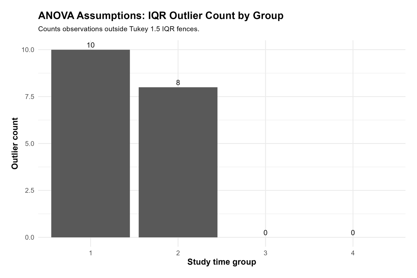
This R chart labels the outlier count by group. Studytime group 1 has 10 outliers, group 2 has 8, group 3 has 0, and group 4 has 0.
The count confirms that all detected IQR outliers are in the first two studytime groups. This explains why the residual plots have a strong lower-tail problem while the variance test remains non-significant.
In reporting, say that 18 IQR outliers were detected, all in studytime groups 1 and 2. These cases should be checked as part of the diagnostic review and should not be removed unless there is a clear data or design reason.
SPSS Output Interpretation for ANOVA Assumptions
The SPSS output PDF should be used as the final software verification file for the ANOVA Assumptions workflow. It should include descriptive group output, assumption checks, residual diagnostics, homogeneity evidence and the exported output used for reporting.
Download ANOVA Assumptions SPSS Output PDF
SPSS Output Items to Read
| SPSS Output Item | What It Shows | How It Is Used | Reporting Meaning |
|---|---|---|---|
| Descriptives | Group n, mean, standard deviation and confidence interval. | Shows the direction and size of group mean differences. | Report group means before the ANOVA test. |
| Test of Homogeneity of Variances | Levene statistic and p value. | Checks whether group variances are similar. | State whether equal variance was supported. |
| ANOVA table | Between-group and within-group F test. | Tests whether group means differ. | Report F, df and p value. |
| Residual histogram | Residual distribution shape. | Checks whether residuals are centered and approximately normal. | Report center and tail behavior. |
| Residual Q-Q plot | Residual normality pattern. | Shows whether points follow a normal reference line. | Report central fit and tail departures. |
| Boxplot and outlier review | Spread and unusual values by group. | Shows whether outliers are concentrated in particular groups. | Report outlier review before final decision. |
SPSS PDF: Final Verification
The ANOVA Assumptions SPSS Output PDF should be used as the final verification file for SPSS results. The PDF gives readers a direct way to check the software output behind the article, including homogeneity evidence, residual diagnostics and final assumption reporting.
In the final article, the PDF should be placed in the downloads section and mentioned in the SPSS interpretation section. The strongest SPSS-style conclusion is that equal variance is supported, while residual tail departures and low-score outliers should be transparently discussed.
SPSS Reporting Summary
The SPSS report should state that ANOVA assumptions were checked using group descriptives, boxplots, residual plots, Q-Q plot and homogeneity testing. The Levene result supports equal variances, while the residual and outlier plots show lower-tail cases in the lower studytime groups.
A correct SPSS-style assumption sentence is: “Levene’s test was not significant, p = .380, supporting homogeneity of variance. Residual plots were centered near zero, although Q-Q and histogram diagnostics showed lower-tail departures caused by low-score outliers, mainly in studytime groups 1 and 2.”
SPSS, R, Python and Excel Workflows for ANOVA Assumptions
The same ANOVA assumptions can be checked in SPSS, R, Python and Excel. The software changes, but the reporting logic stays the same: describe group means, inspect group spread, test equal variance, inspect residual shape and review outliers.
SPSS Workflow
| Step | SPSS Menu or Syntax | Purpose |
|---|---|---|
| Open data | File > Open > Data | Load the dataset with G3 and studytime. |
| Run one-way ANOVA | Analyze > Compare Means > One-Way ANOVA | Compare G3 means across studytime groups. |
| Request descriptives | Options > Descriptive | Get group mean, SD and confidence interval. |
| Request homogeneity test | Options > Homogeneity of variance test | Get Levene’s test. |
| Use Explore | Analyze > Descriptive Statistics > Explore | Generate boxplots, histograms and Q-Q plots. |
| Export output | Output Export to PDF | Save SPSS results for documentation. |
R Workflow
| Step | R Action | Purpose |
|---|---|---|
| Read data | read.csv("dataset.csv") | Load the dataset. |
| Set factor | df$studytime <- as.factor(df$studytime) | Define the grouping variable. |
| Fit ANOVA | aov(G3 ~ studytime, data = df) | Fit the one-way ANOVA model. |
| Residual checks | plot(model) | Generate residual diagnostic plots. |
| Levene test | car::leveneTest(G3 ~ studytime, data=df) | Check homogeneity of variance. |
| Outlier count | IQR rule by group | Count possible outliers in each group. |
Python Workflow
| Step | Python Action | Purpose |
|---|---|---|
| Read data | pandas.read_csv() | Load the dataset. |
| Fit model | ols("G3 ~ C(studytime)", data=df).fit() | Fit the ANOVA model. |
| ANOVA table | sm.stats.anova_lm(model, typ=2) | Get F test output. |
| Residual diagnostics | Histogram, Q-Q plot, residuals vs fitted | Check residual normality and pattern. |
| Levene test | scipy.stats.levene() | Check equal variance assumption. |
| Outlier review | IQR rule by group | Count group-specific outliers. |
Excel Workflow
| Excel Task | Formula or Tool | Purpose |
|---|---|---|
| Group mean | =AVERAGE(group_range) | Calculate each studytime group mean. |
| Group standard deviation | =STDEV.S(group_range) | Compare group spread. |
| One-way ANOVA | Data Analysis ToolPak > ANOVA: Single Factor | Run the F test. |
| Residuals | =Observed_G3 - Group_Mean | Create residual values. |
| Outlier fences | Q1 - 1.5*IQR and Q3 + 1.5*IQR | Identify IQR outliers. |
| Residual histogram | Insert > Statistic Chart > Histogram | Check residual distribution shape. |
Code Blocks for ANOVA Assumptions
SPSS Syntax for ANOVA Assumptions
* ANOVA Assumptions in SPSS.
* Dependent variable: G3.
* Grouping factor: studytime.

TITLE "ANOVA Assumptions: G3 by Studytime".

ONEWAY G3 BY studytime
  /STATISTICS DESCRIPTIVES HOMOGENEITY
  /MISSING ANALYSIS.

EXAMINE VARIABLES=G3 BY studytime
  /PLOT BOXPLOT HISTOGRAM NPPLOT
  /STATISTICS DESCRIPTIVES
  /CINTERVAL 95
  /MISSING LISTWISE
  /NOTOTAL.

UNIANOVA G3 BY studytime
  /METHOD=SSTYPE(3)
  /INTERCEPT=INCLUDE
  /PRINT=DESCRIPTIVE HOMOGENEITY ETASQ
  /SAVE=PRED RESID
  /CRITERIA=ALPHA(.05)
  /DESIGN=studytime.

EXAMINE VARIABLES=RES_1
  /PLOT HISTOGRAM NPPLOT
  /STATISTICS DESCRIPTIVES
  /CINTERVAL 95
  /MISSING LISTWISE.

OUTPUT EXPORT
  /CONTENTS EXPORT=VISIBLE
  /PDF DOCUMENTFILE="ANOVA-Assumptions-SPSS-Output.pdf".
Python Code for ANOVA Assumptions
import pandas as pd
import scipy.stats as stats
import statsmodels.api as sm
from statsmodels.formula.api import ols

df = pd.read_csv("dataset.csv")

df["G3"] = pd.to_numeric(df["G3"], errors="coerce")
df["studytime"] = df["studytime"].astype("category")

df_model = df.dropna(subset=["G3", "studytime"])

model = ols("G3 ~ C(studytime)", data=df_model).fit()
anova_table = sm.stats.anova_lm(model, typ=2)

residuals = model.resid
fitted = model.fittedvalues

groups = [
    group["G3"].dropna().values
    for name, group in df_model.groupby("studytime")
]

levene_stat, levene_p = stats.levene(*groups, center="median")
shapiro_stat, shapiro_p = stats.shapiro(residuals)

print(anova_table)
print("Levene statistic:", levene_stat)
print("Levene p value:", levene_p)
print("Shapiro statistic:", shapiro_stat)
print("Shapiro p value:", shapiro_p)

summary = df_model.groupby("studytime")["G3"].agg(["count", "mean", "std", "var"])
print(summary)

# IQR outlier count by group
def count_iqr_outliers(x):
    q1 = x.quantile(0.25)
    q3 = x.quantile(0.75)
    iqr = q3 - q1
    lower = q1 - 1.5 * iqr
    upper = q3 + 1.5 * iqr
    return ((x < lower) | (x > upper)).sum()

outlier_counts = df_model.groupby("studytime")["G3"].apply(count_iqr_outliers)
print(outlier_counts)
R Code for ANOVA Assumptions
df <- read.csv("dataset.csv")

df$G3 <- as.numeric(df$G3)
df$studytime <- as.factor(df$studytime)

df_model <- na.omit(df[, c("G3", "studytime")])

model <- aov(G3 ~ studytime, data = df_model)

summary(model)

aggregate(G3 ~ studytime, data = df_model, FUN = function(x) {
  c(n = length(x), mean = mean(x), sd = sd(x), variance = var(x))
})

# Residual normality check
shapiro.test(residuals(model))

# Levene test
library(car)
leveneTest(G3 ~ studytime, data = df_model)

# IQR outlier count by group
iqr_count <- function(x) {
  q1 <- quantile(x, .25)
  q3 <- quantile(x, .75)
  iqr <- q3 - q1
  lower <- q1 - 1.5 * iqr
  upper <- q3 + 1.5 * iqr
  sum(x < lower | x > upper)
}

aggregate(G3 ~ studytime, data = df_model, FUN = iqr_count)

# Diagnostic plots
par(mfrow = c(2, 2))
plot(model)
Excel Formulas for ANOVA Assumptions
Group mean:
=AVERAGE(group_range)

Group standard deviation:
=STDEV.S(group_range)

Group variance:
=VAR.S(group_range)

Group count:
=COUNT(group_range)

Residual for each observation:
=Observed_G3 - Group_Mean

Variance ratio quick check:
=MAX(group_variance_range)/MIN(group_variance_range)

Lower outlier fence:
=Q1 - 1.5*IQR

Upper outlier fence:
=Q3 + 1.5*IQR

Outlier flag:
=IF(OR(valueupper_fence),"Review","OK")

ANOVA:
Data > Data Analysis > ANOVA: Single Factor
APA Reporting Wording
When reporting ANOVA Assumptions, include the grouping factor, dependent variable, normality check, homogeneity check and outlier review. The assumption paragraph should appear before or immediately after the ANOVA F test.
APA-style assumption report: ANOVA assumptions were examined before interpreting the group comparison. G3 final grade was compared across four studytime groups. Levene’s test was not significant, p = .380, supporting homogeneity of variance. Residual plots showed values centered near zero, although the histogram and Q-Q plot showed lower-tail departures. IQR outlier review identified 10 outliers in studytime group 1 and 8 in group 2, with no detected IQR outliers in groups 3 or 4.
Short reporting version: Levene’s test supported homogeneity of variance, p = .380. Residual diagnostics were mostly centered but showed lower-tail departures, and IQR outliers were concentrated in studytime groups 1 and 2.
Common Mistakes
| Mistake | Why It Is Wrong | Correct Practice |
|---|---|---|
| Checking only raw-variable normality | ANOVA mainly uses residual normality, not perfect raw normality. | Check residual histogram and residual Q-Q plot. |
| Ignoring Levene’s test | Unequal variances can distort the ordinary F test. | Report Levene’s homogeneity result. |
| Saying assumptions are perfect | Residual plots often show some departures. | Report the actual diagnostic pattern. |
| Deleting outliers automatically | Outliers may be valid observations. | Review, verify and run sensitivity checks if needed. |
| Confusing boxplot outliers with errors | Boxplot outliers are diagnostic flags, not proof of bad data. | Check original records and context. |
| Using ordinary ANOVA after severe variance violation | Strong heterogeneity can affect the F test. | Use Welch-style methods, Brown-Forsythe Test or robust alternatives when needed. |
When to Check ANOVA Assumptions
Check ANOVA assumptions every time a mean comparison is reported with ANOVA. The same logic applies to one-way ANOVA, two-way ANOVA, repeated measures ANOVA and ANCOVA-style models, although repeated measures and ANCOVA have additional assumptions.
| Analysis Type | Assumptions to Check | Useful Diagnostic Output |
|---|---|---|
| One-way ANOVA | Independence, residual normality, equal variances and outliers. | Boxplots, Levene test, residual histogram and Q-Q plot. |
| Two-way ANOVA | Same assumptions plus factor-combination adequacy. | Residual plots, cell-size review and homogeneity checks. |
| Repeated measures ANOVA | Normality and sphericity. | Mauchly’s Test of Sphericity, Greenhouse-Geisser Correction and Huynh-Feldt Correction. |
| ANCOVA | ANOVA assumptions plus covariate linearity and homogeneous slopes. | Residual plots, group × covariate interaction and adjusted means. |
For t-test and z-test comparisons that connect to ANOVA thinking, see T Test vs ANOVA, T Test Assumptions, Independent Samples T Test, Two Sample T Test, T Test for Equal Variances, T Test for Unequal Variances, T Test in Python, T Test in R, T Test in SPSS, and T Test in Excel.
Downloads and Resources for ANOVA Assumptions
The SPSS output PDF below verifies the ANOVA Assumptions workflow, including group summaries, homogeneity evidence, residual diagnostics and outlier review. Replace placeholder script links with final uploaded files after the dataset, Python script, R script, SPSS syntax and Excel workbook are uploaded to WordPress Media Library.
Download Dataset
Practice dataset with G3 and studytime variables.
Download ANOVA Assumptions SPSS Output PDF
SPSS output PDF for ANOVA assumption checks and reporting.
Download Python Script
Python code for group means, residual diagnostics, Levene test and charts.
Download R Script and Excel Workbook
R validation code and Excel formulas for ANOVA assumption checking.
FAQs About ANOVA Assumptions
What are ANOVA assumptions?
ANOVA assumptions are the diagnostic conditions needed before interpreting an ANOVA F test. They include independent observations, a numeric dependent variable, approximate residual normality, similar group variances and outlier review.
What are the assumptions of one-way ANOVA?
One-way ANOVA assumes independent observations, one numeric outcome, one categorical grouping factor, approximately normal residuals and similar group variances.
What are the assumptions of two-way ANOVA?
Two-way ANOVA has the same basic assumptions as one-way ANOVA, but the analyst should also check the factor-combination structure, interaction pattern and cell sizes.
How do I check ANOVA assumptions?
Use group means, boxplots, residual histogram, residual Q-Q plot, residuals versus fitted values, Levene’s test and outlier counts by group.
What does Levene’s test check in ANOVA?
Levene’s test checks whether the group variances are similar. In this example, p = .3804, so the homogeneity of variance assumption is supported.
Does ANOVA require perfect normality?
No. ANOVA mainly requires approximately normal residuals. Mild departures are often acceptable, especially with larger samples, but strong tail departures should be reported.
What should I do if ANOVA has outliers?
Outliers should be reviewed, verified and reported. They should not be deleted automatically. Sensitivity analysis or robust methods can be used if outliers strongly affect the result.
How do I report ANOVA assumptions in APA format?
Report the homogeneity test, residual normality check and outlier review. For this example, Levene’s test was not significant, p = .380, residuals were centered but showed lower-tail departures, and outliers were concentrated in groups 1 and 2.
What if Levene’s test is significant?
If Levene’s test is significant, the equal-variance assumption may be violated. Consider Welch ANOVA, Brown-Forsythe ANOVA, robust ANOVA or transformation methods.
Can I use ANOVA if residual Q-Q plot is not perfect?
Yes, if departures are mild and the sample size is reasonable. In this example, the center of the Q-Q plot is acceptable, but lower-tail departures should be reported as a diagnostic caution.

