
Directional Hypothesis Testing, Right-Tailed Decision, Rejection Region and One-Sided Confidence Bound
One Tailed T Test: Formula, Interpretation, SPSS, Python, R and Excel Guide
One Tailed T Test is used when the research hypothesis is directional before analysis. Instead of asking whether a sample mean is simply different from a null value, a One Tailed T Test asks whether the sample mean is significantly greater than or significantly less than the null boundary. This guide explains a right-tailed One Tailed T Test with actual G3 final grade data, SPSS output interpretation, Python charts, R validation charts, Excel workflow, code blocks, APA wording, common mistakes, downloadable resources, related guides and FAQ schema.
Quick Answer: One Tailed T Test Result
The worked One Tailed T Test used a right-tailed directional hypothesis: H1: μ > 10. The test compared the average G3 final grade with the null boundary of 10.000. The sample mean was 11.906, which is 1.906 grade points higher than the null boundary.
The observed test statistic was t(648) = 15.03. The right-tail critical value at the 5% level was approximately 1.65. Since the observed t statistic is far greater than the critical t value, the result falls deep inside the right-tailed rejection region. The one-tailed p value is p < .001, so the null hypothesis is rejected.
Final interpretation: The right-tailed One Tailed T Test supports the directional claim that the mean G3 final grade is greater than 10. The sample mean is higher than the null boundary, the t statistic is far beyond the right-tail critical value, and the lower one-sided 95% confidence bound is also above 10.
Important reporting point: A one-tailed test must be justified before looking at the data. Do not choose a one-tailed test only because the sample mean moved in a preferred direction. If the direction was not specified in advance, use a two-tailed test instead.
Table of Contents
- What Is a One Tailed T Test?
- One Tailed T Test Formula
- Null and Alternative Hypothesis
- Dataset and Test Variable Used
- SPSS Output Interpretation
- Python Chart-by-Chart Interpretation
- R Chart-by-Chart Validation
- SPSS, R, Python and Excel Workflows
- Code Blocks for One Tailed T Test
- APA Reporting Wording
- Common Mistakes
- When to Use One Tailed T Test
- Downloads and Resources
- Related Guides
- FAQs
What Is a One Tailed T Test?
A One Tailed T Test is a directional version of a t test. It tests whether a mean is significantly greater than a null value or significantly less than a null value. The key feature is direction. A right-tailed test asks whether the mean is greater than the null boundary. A left-tailed test asks whether the mean is less than the null boundary.
In this example, the research question is right-tailed: Is the average G3 final grade greater than 10? The null boundary is 10.000. The observed sample mean is 11.906. Because the sample mean is above the null boundary, the direction of the data is consistent with the right-tailed alternative hypothesis.
A One Tailed T Test is not simply a shortcut for making results significant. It is only appropriate when the researcher has a directional hypothesis before seeing the data and when an effect in the opposite direction would not support the research claim. If both directions matter, the correct test is a two-tailed t test.
Simple definition: A One Tailed T Test checks whether a sample mean is significantly higher than a null value or significantly lower than a null value. In this post, the right-tailed version tests whether μ > 10.
One Tailed T Test interpretation belongs inside a broader hypothesis-testing workflow. It should be interpreted together with the directional hypothesis, sample mean, null boundary, standard error, t statistic, critical value, p value, one-sided confidence bound and effect size. Useful related guides include Null and Alternative Hypothesis, P Value, Confidence Interval, Effect Size, and Standard Error.
One Tailed T Test Formula
The test statistic for a One Tailed T Test uses the same t formula as a one-sample t test. The difference is the direction of the rejection region and the p value interpretation.
For a right-tailed test, the alternative hypothesis is:
The directional mean difference for this example is:
The degrees of freedom are:
| Symbol | Meaning | Value in This Example |
|---|---|---|
| x̄ | Sample mean | 11.906 |
| μ0 | Null boundary or test value | 10.000 |
| s | Sample standard deviation | Approximately 3.23 |
| n | Sample size | 649 |
| s / √n | Standard error | Approximately 0.127 |
| t | Observed test statistic | 15.03 |
| df | Degrees of freedom | 648 |
| tcritical | Right-tail critical value at α = .05 | Approximately 1.65 |
Threshold rule: For a right-tailed test, reject the null hypothesis when the observed t statistic is greater than the right-tail critical value. Here, 15.03 > 1.65, so the result is strongly significant.
Null and Alternative Hypothesis for One Tailed T Test
The One Tailed T Test must have a directional alternative hypothesis. In this example, the direction is right-tailed because the research question asks whether the mean G3 score is greater than 10.
| Statement | Hypothesis | Meaning |
|---|---|---|
| Null hypothesis | H0: μ ≤ 10 | The population mean G3 final grade is not greater than 10. |
| Right-tailed alternative | H1: μ > 10 | The population mean G3 final grade is greater than 10. |
| Observed direction | x̄ = 11.906 > 10 | The sample mean supports the right-tailed direction. |
Decision for this example: The null hypothesis is rejected because t(648) = 15.03 is far greater than the right-tail critical value of approximately 1.65, and the one-tailed p value is p < .001. The data support the claim that mean G3 is greater than 10.
Dataset and Test Variable Used
The worked example uses a student performance dataset. The test variable is G3 final grade. The null boundary is set to 10.000. The directional hypothesis asks whether the population mean G3 score is greater than 10.
| Variable or Value | Role | Why It Matters for One Tailed T Test |
|---|---|---|
| G3 | Test variable | The final grade whose mean is tested against the null boundary. |
| 10.000 | Null boundary | The benchmark value used in the right-tailed hypothesis. |
| 649 | Sample size | Large sample size gives a precise estimate of the mean. |
| 11.906 | Sample mean | The observed average final grade in the sample. |
| School | Context variable | Used in a descriptive chart to show how G3 differs by school group. |
Before interpreting a One Tailed T Test, it is useful to understand the distribution of the test variable using descriptive statistics, frequency distributions, histograms, box plots, and the five-number summary.
SPSS Output Interpretation for One Tailed T Test
SPSS usually reports the one-sample t test with a two-tailed significance value. For a planned right-tailed test, the analyst must interpret the output directionally. If the sample mean is in the hypothesized direction, the one-tailed p value is usually half of the two-tailed p value. In this example, the result is so strong that the one-tailed p value is still reported as p < .001.
SPSS One-Sample Statistics
| SPSS Output Item | Value | Interpretation |
|---|---|---|
| Test variable | G3 | The final grade variable is tested. |
| N | 649 | There are 649 valid G3 scores. |
| Mean | 11.906 | The observed average G3 score is above the null boundary. |
| Std. Deviation | Approximately 3.23 | G3 scores vary by about 3.23 points around the mean. |
| Std. Error Mean | Approximately 0.127 | The sample mean is estimated precisely because the sample size is large. |
SPSS One-Sample Test Converted to Right-Tailed Interpretation
| SPSS Output Item | Value | Right-Tailed Interpretation |
|---|---|---|
| Test value | 10.000 | The null boundary for the right-tailed test. |
| t | 15.03 | The observed t value is far inside the right-tailed rejection region. |
| df | 648 | Degrees of freedom are calculated as n − 1. |
| Right-tail critical t | Approximately 1.65 | The observed t value is much greater than the critical value. |
| One-tailed p value | < .001 | The directional result is statistically significant. |
| Mean difference | 1.906 | The sample mean is 1.906 points higher than 10. |
| Lower one-sided 95% confidence bound | 11.697 | The population mean is estimated to be above 11.697 with one-sided 95% confidence. |
SPSS Directional Decision Interpretation
The SPSS-style result supports the right-tailed hypothesis because the mean difference is positive, the observed t statistic is positive and very large, and the lower one-sided confidence bound is above the null boundary. The conclusion is not merely that G3 differs from 10; the directional conclusion is that mean G3 is significantly greater than 10.
SPSS interpretation summary: A right-tailed one-sample t test showed that the mean G3 score was significantly greater than 10, M = 11.906, t(648) = 15.03, p < .001. The observed mean difference was 1.906, and the lower one-sided 95% confidence bound for the mean was 11.697.
Python Chart-by-Chart Interpretation
The Python charts below show the complete One Tailed T Test workflow. They include the G3 distribution with the null boundary and sample mean, the sample mean versus null boundary comparison, the directional mean difference, the one-tailed rejection region, the one-sided confidence bound, the boxplot with null boundary, and the school-level context chart. Additional Python output charts are also included to preserve all provided output images.
Python Chart 1: G3 Distribution with Null Boundary and Sample Mean
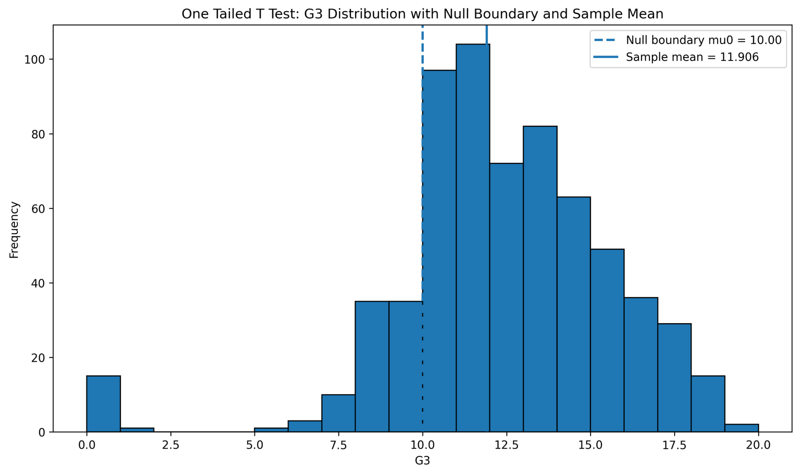
This distribution chart shows the observed G3 final grade values with two important vertical lines. The dashed line marks the null boundary at 10.000, and the solid line marks the sample mean at 11.906. The sample mean is clearly to the right of the null boundary, which supports the right-tailed direction.
The chart also shows that the distribution is concentrated around scores above 10, although there are some lower-end values. For a right-tailed test, the important point is whether the sample mean is sufficiently above the null boundary. The formal t statistic confirms that the difference is statistically significant.
Python Chart 2: Sample Mean Compared with Null Boundary
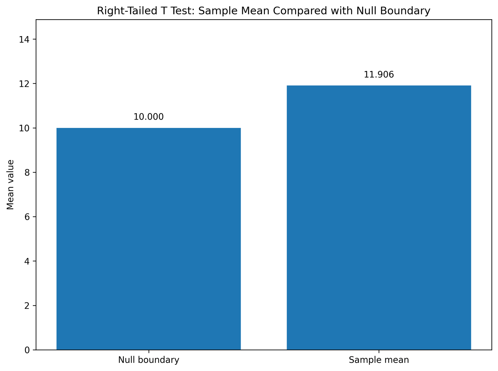
This chart turns the directional hypothesis into a simple visual comparison. The null boundary is 10.000, while the sample mean is 11.906. The sample mean is higher than the null boundary, so the observed direction supports H1: μ > 10.
This visual is useful for nontechnical readers because it shows the main directional result before the t statistic is discussed. The difference is not just positive; it is large enough to produce a very large observed t value.
Python Chart 3: Directional Mean Difference from Null Boundary
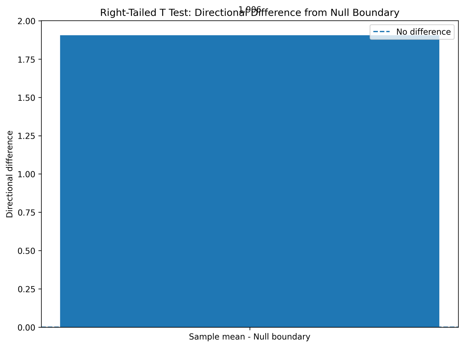
This chart focuses on the mean difference itself. The directional difference is 1.906, calculated as sample mean minus null boundary. Since the value is positive, it supports a right-tailed alternative.
The chart is important because the practical size of the result should be reported along with the p value. In the original G3 scale, the sample mean is almost two points above the benchmark.
Python Chart 4: One-Tailed Rejection Region on Student’s t Distribution
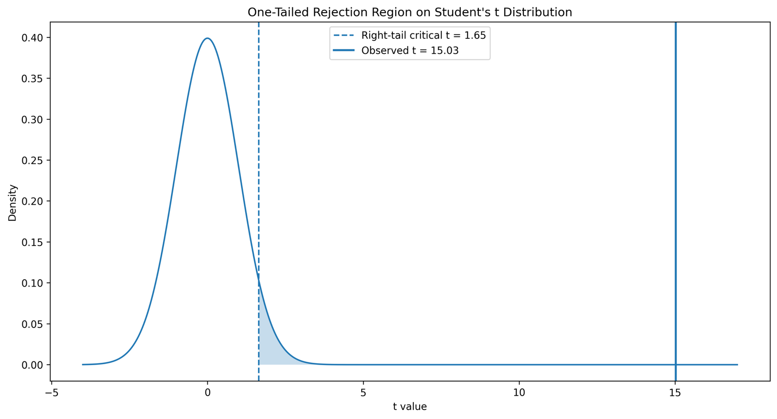
This is the central inferential chart. The right-tailed critical value is approximately 1.65, while the observed test statistic is 15.03. The observed t statistic is far to the right of the rejection boundary.
This chart explains why the p value is extremely small. Under the null hypothesis, a t statistic this far into the right tail would be extremely unlikely. Therefore, the directional null hypothesis is rejected.
Python Chart 5: One-Sided Confidence Bound for Mean G3
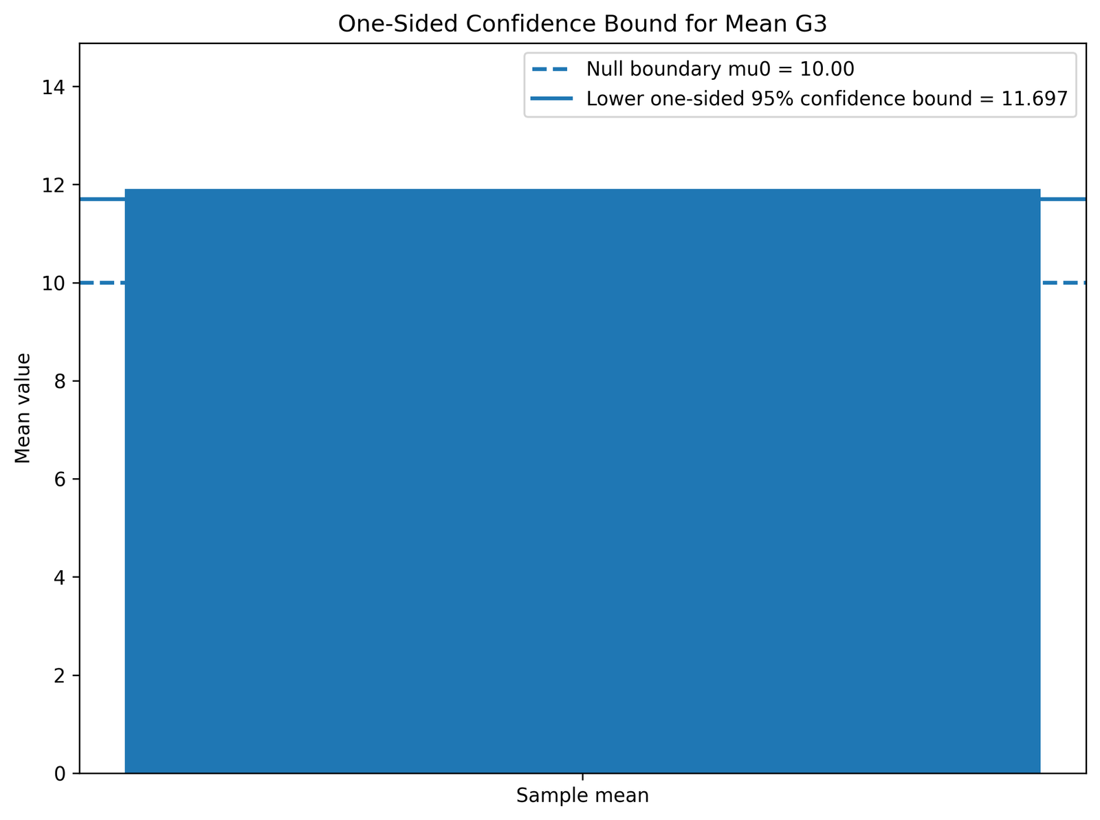
The one-sided confidence bound chart shows that the lower one-sided 95% confidence bound is 11.697. This bound is above the null boundary of 10.000.
This supports the right-tailed conclusion from another angle. Instead of asking whether the mean is different, the one-sided confidence statement says that the population mean is confidently above a value that is already higher than the null boundary.
Python Chart 6: Boxplot of G3 with Null Boundary
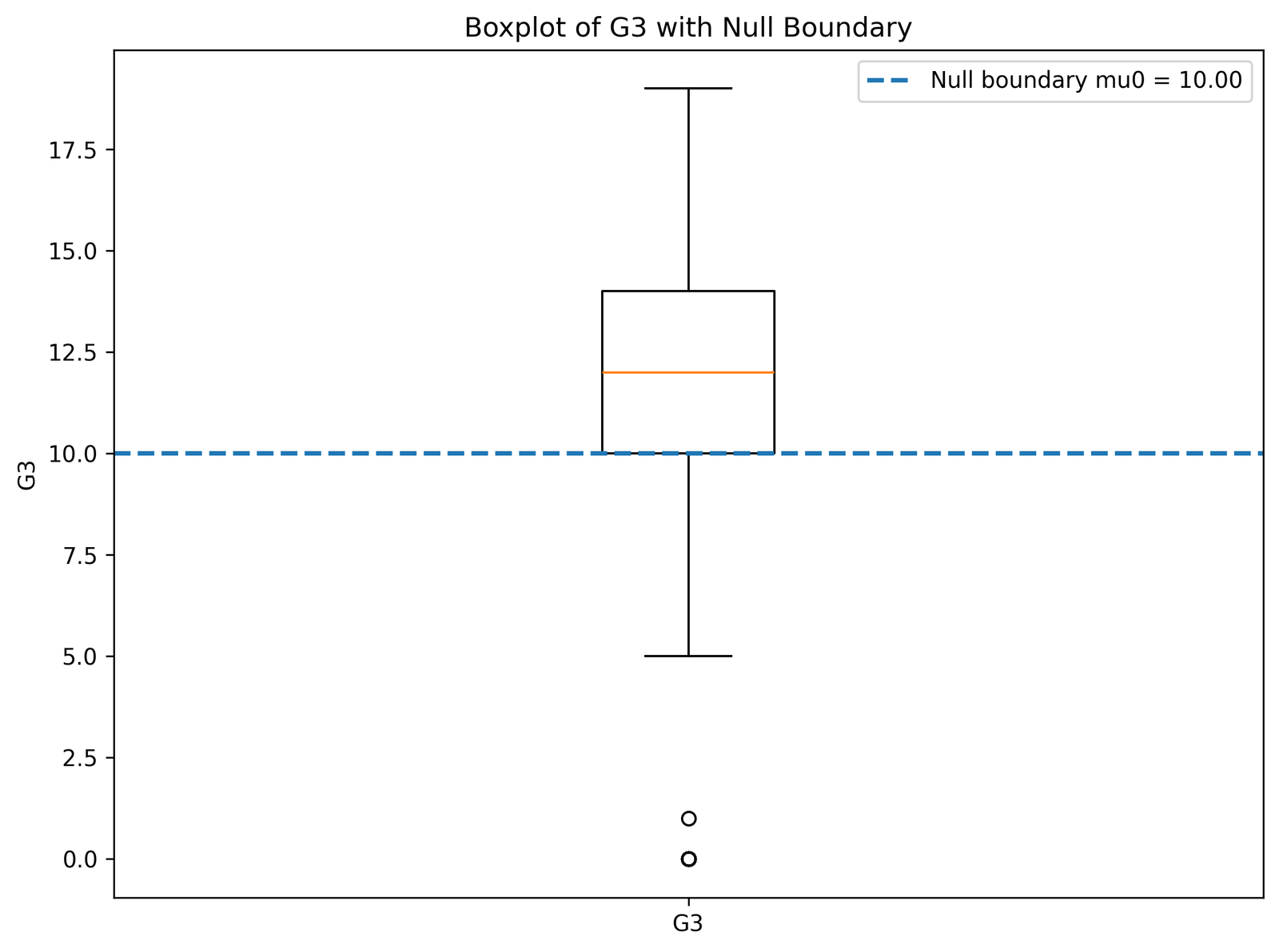
The boxplot shows the center and spread of G3 values. The median is above the null boundary, and much of the box lies at or above 10. This supports the directional interpretation that the typical G3 score is above the benchmark.
The chart also shows a few low-end values, including very low scores. These values should be acknowledged, but they do not overturn the result because the sample mean, rejection-region chart and confidence bound all support the right-tailed conclusion.
Python Chart 7: Mean G3 by School for One-Tailed Context
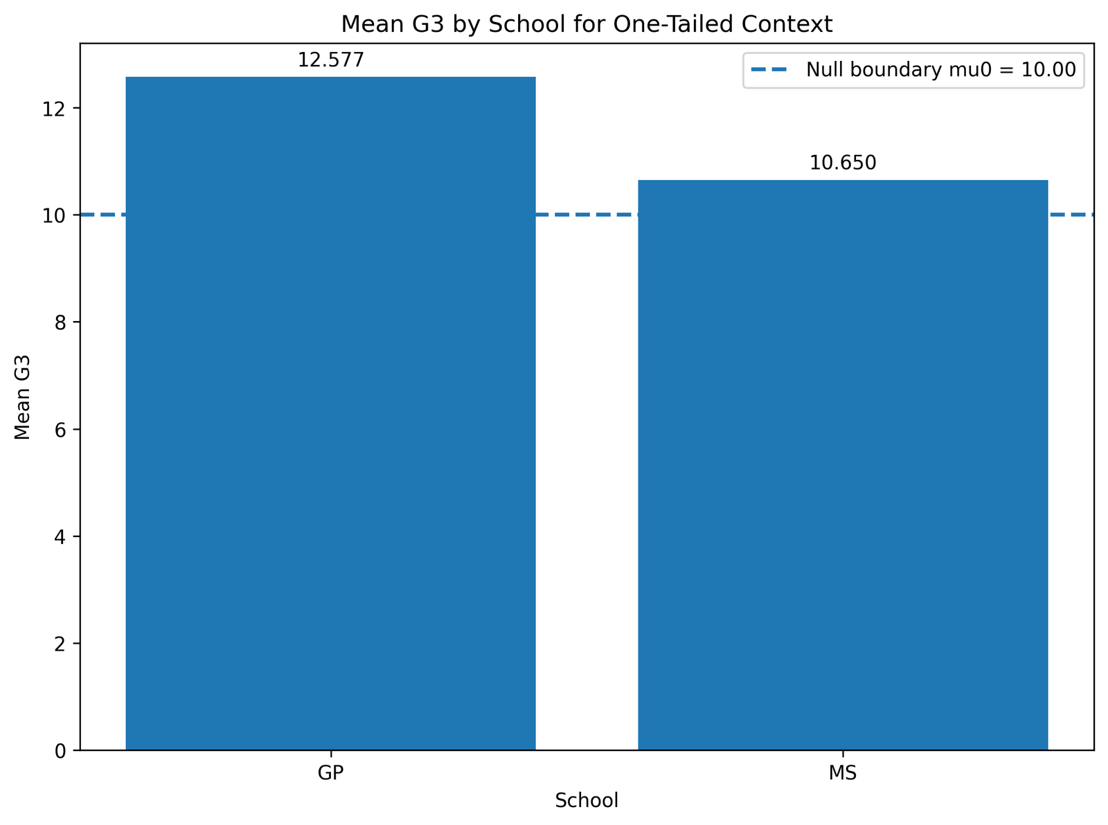
This context chart shows the mean G3 score by school. The GP mean is 12.577, and the MS mean is 10.650. Both school-level means are above the null boundary of 10.000.
This chart does not replace the one-tailed t test because the main test is based on the overall sample mean. However, it helps explain why the overall sample mean is greater than 10: both school groups are above the benchmark.
Python Chart 8: Additional G3 Distribution Output
This additional output image preserves the supplied chart set and supports the same distribution-based interpretation. The chart represents the same idea: the G3 distribution is evaluated against a null boundary and a sample mean.
Even when the export style is minimal, the purpose remains the same. It provides an additional visual output for the one-tailed workflow and should be kept with the post assets.
Python Chart 9: Additional Sample Mean vs Null Boundary Output
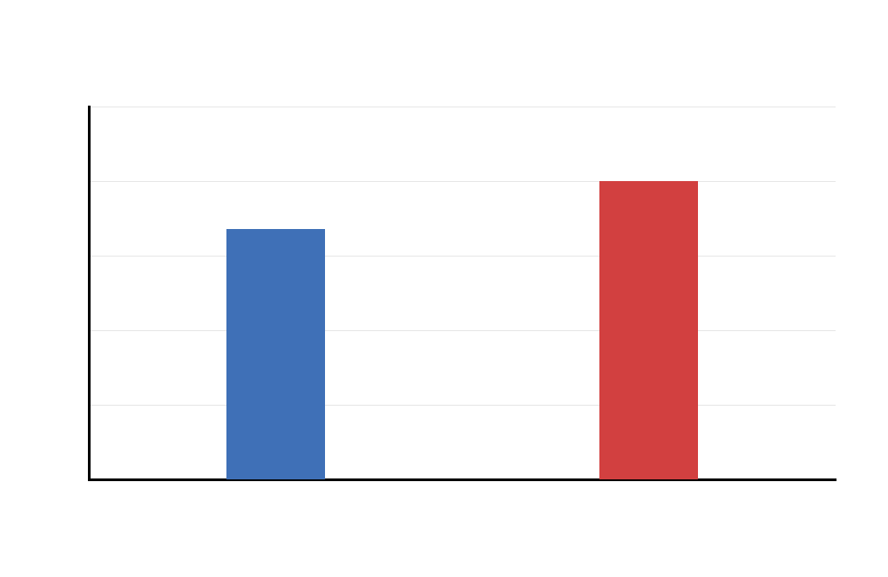
This additional chart repeats the sample mean versus null boundary comparison. It reinforces the same directional story: the observed sample mean is above the null boundary.
The chart is included as part of the complete output set and can be used as an alternate image export for visual verification.
Python Chart 10: Additional Directional Mean Difference Output
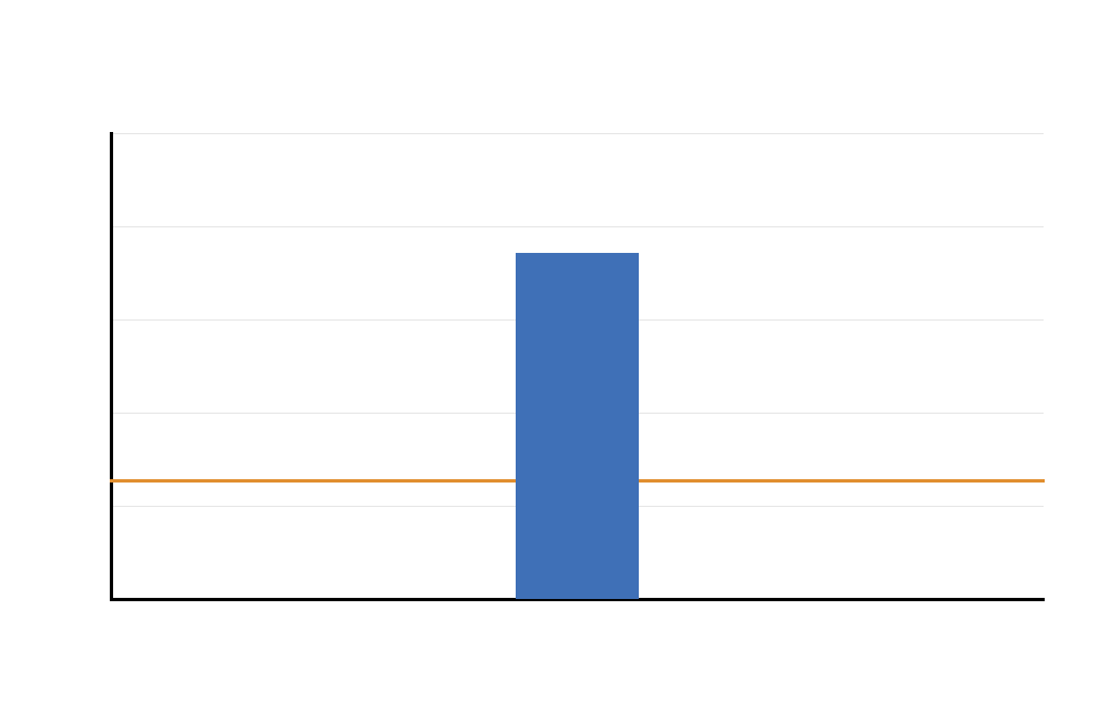
This additional chart repeats the directional mean difference output. The positive value supports the right-tailed alternative hypothesis.
It also reinforces the practical interpretation: the sample mean is above the null boundary by about 1.906 G3 points.
R Chart-by-Chart Validation
The R charts validate the Python and SPSS conclusions using a separate workflow. The R visual pattern is the same: the sample mean is higher than the null boundary, the directional mean difference is positive, the observed t statistic is far beyond the right-tail critical value, the one-sided confidence bound is above the null boundary, and the school context supports the overall direction. This software-to-software agreement strengthens confidence in the interpretation.
R Chart 1: G3 Distribution with Null Boundary and Sample Mean
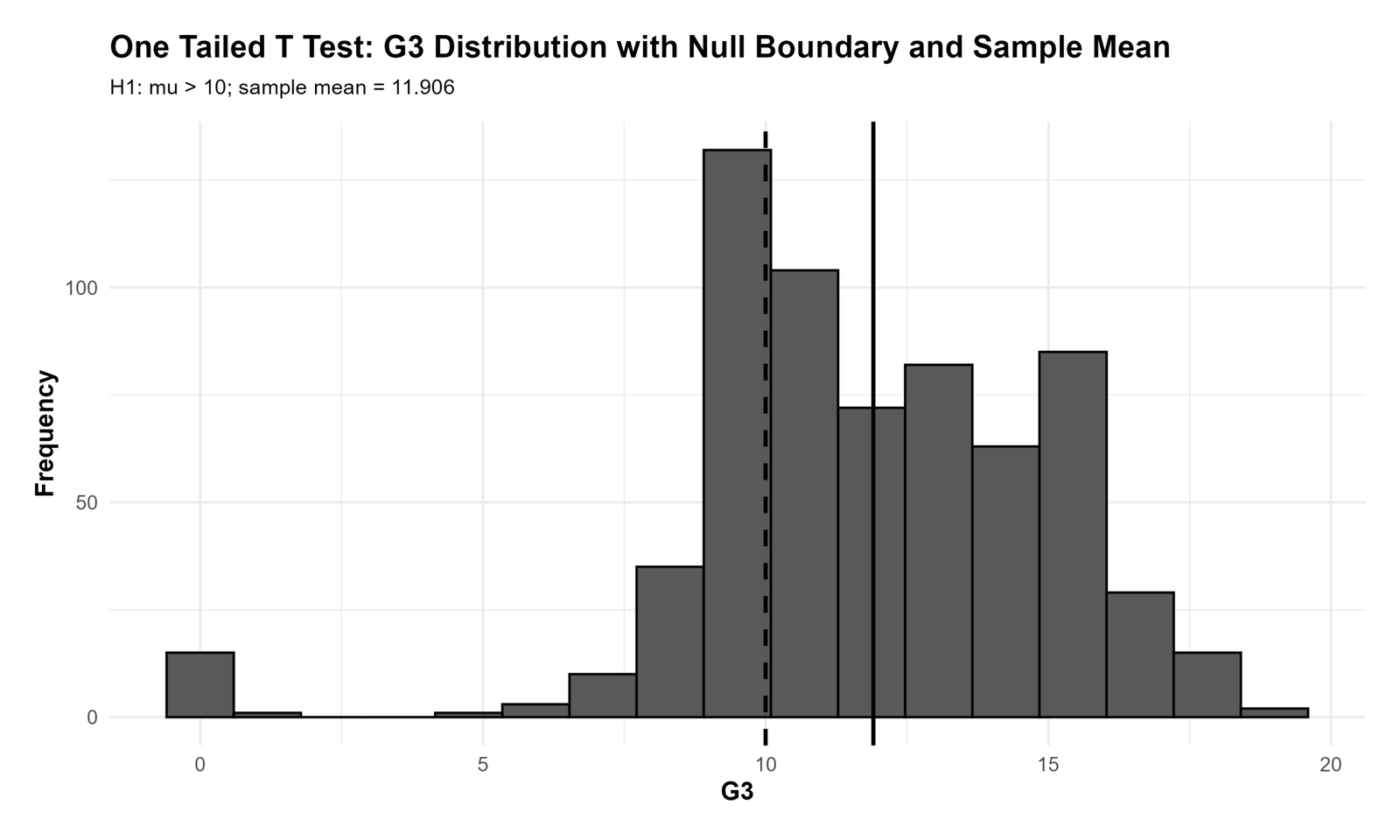
The R distribution chart confirms the same pattern as Python. The dashed null boundary is at 10.000, and the sample mean is marked at 11.906. The sample mean is to the right of the null boundary, which supports the right-tailed hypothesis.
This chart validates that the observed directional result is not a software artifact. Both Python and R show the sample mean above the benchmark.
R Chart 2: Sample Mean Compared with Null Boundary
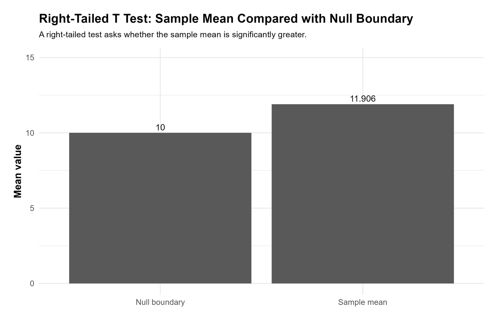
This R chart again shows the main comparison: 10.000 versus 11.906. The sample mean is clearly higher than the null boundary.
The chart is useful for final reporting because it communicates the directional result clearly. The hypothesis is right-tailed, and the observed mean supports that direction.
R Chart 3: Directional Mean Difference from Null Boundary
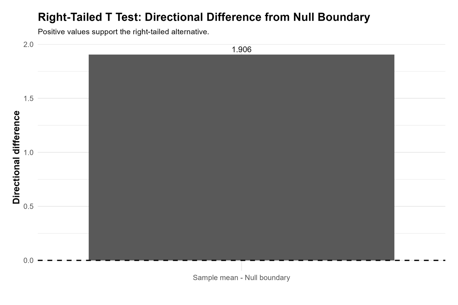
The R mean-difference chart confirms the positive directional difference of 1.906. Positive values support the right-tailed alternative because the sample mean is greater than the null boundary.
This chart is important because it explains the result in the original G3 scale. The test is not only significant; the observed average is about 1.91 points above the benchmark.
R Chart 4: One-Tailed Rejection Region on Student’s t Distribution
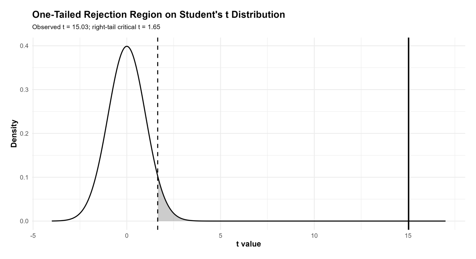
This R chart confirms the inferential decision. The observed t statistic is 15.03, while the right-tail critical value is approximately 1.65. Since the observed t value is far to the right of the critical value, the result falls inside the rejection region.
The shaded right-tail region represents the rejection area for the directional test. The observed statistic is far beyond this area, which explains why the p value is reported as p < .001.
R Chart 5: One-Sided Confidence Bound for Mean G3
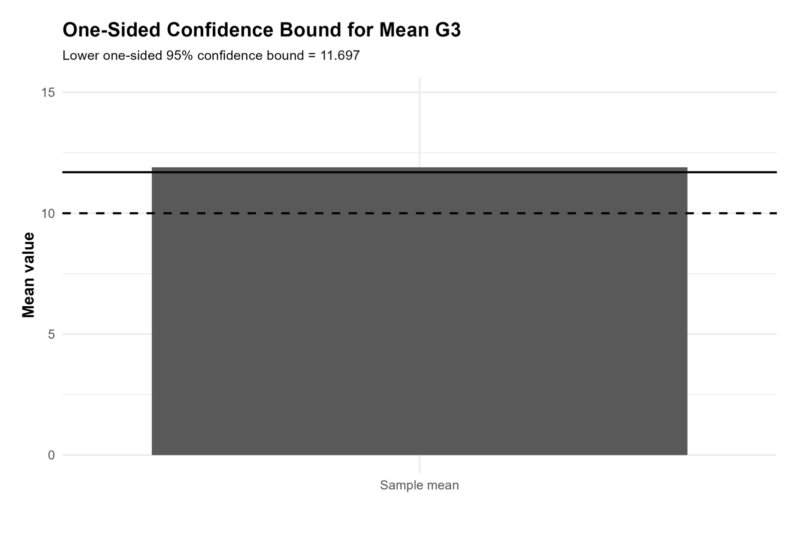
This R chart shows the lower one-sided 95% confidence bound for mean G3. The lower bound is 11.697, which is above the null boundary of 10.000.
This confidence-bound interpretation supports the right-tailed result. If the lower bound is already above 10, the evidence strongly supports the claim that the population mean is greater than 10.
R Chart 6: Boxplot of G3 with Null Boundary
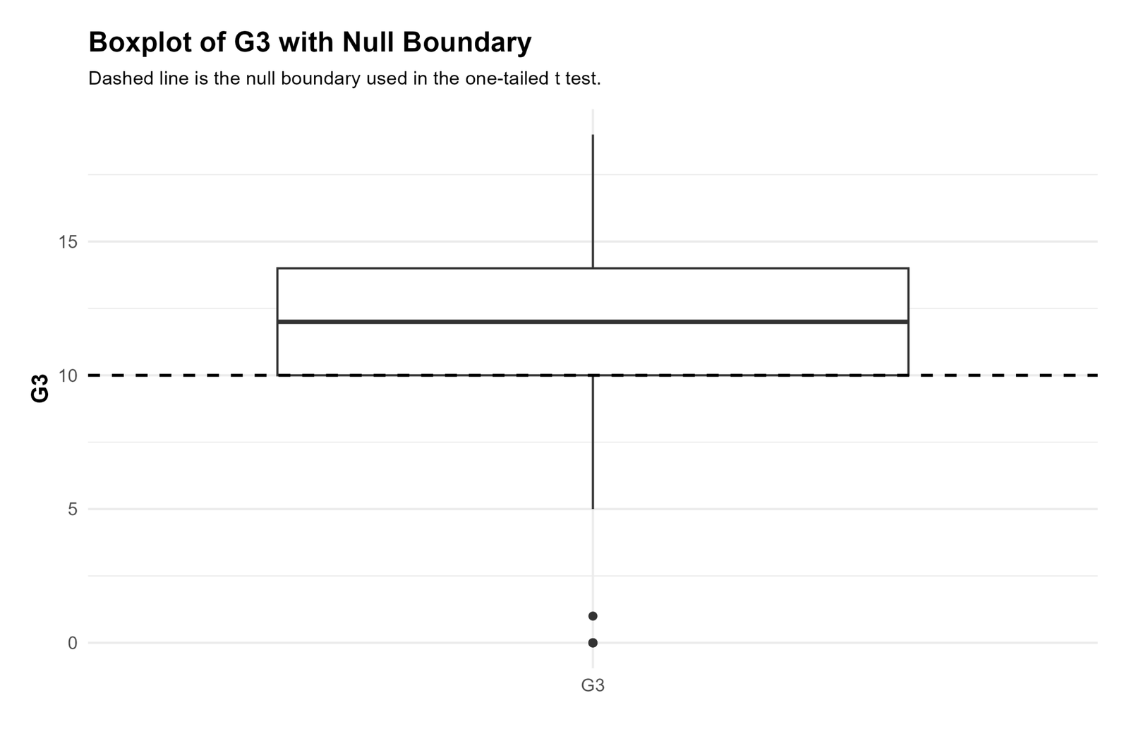
The R boxplot confirms that the center of the G3 distribution is above the null boundary. The median appears above 10, and the upper part of the distribution extends well above the benchmark.
The chart also shows a few lower-end observations. These values should be acknowledged, but they do not change the directional conclusion because the overall mean, t statistic and confidence bound all support μ > 10.
R Chart 7: Mean G3 by School for One-Tailed Context
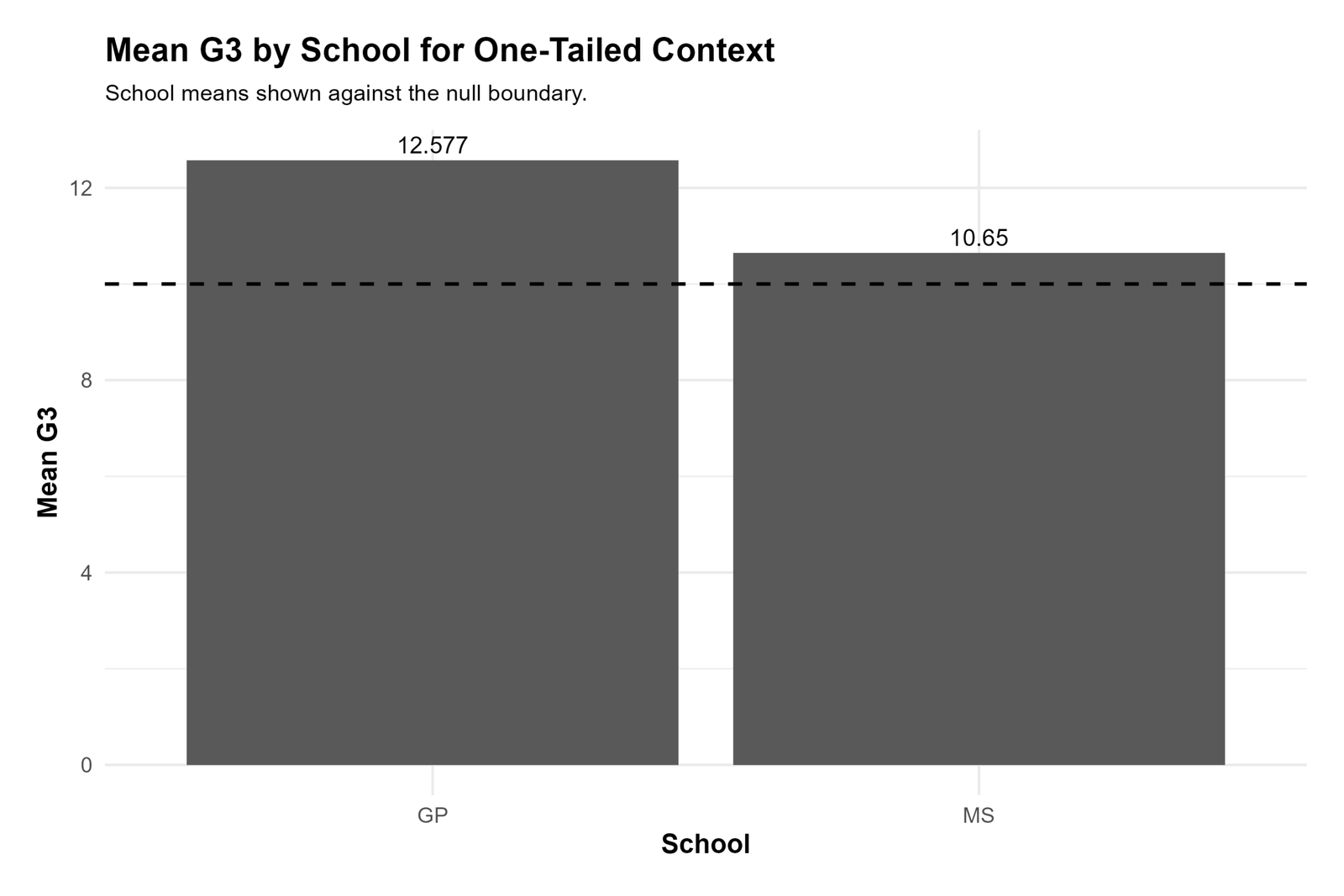
The R school context chart validates the Python school context. The GP mean is 12.577, and the MS mean is 10.650. Both means are above the null boundary.
This chart helps explain why the total sample mean is above 10. The directional result is not driven by only one school group; both displayed school groups are above the benchmark.
SPSS, R, Python and Excel Workflows for One Tailed T Test
The same One Tailed T Test workflow can be reproduced in SPSS, R, Python and Excel. SPSS reports the one-sample t test output, and the researcher converts the significance interpretation to one-tailed only when the direction was specified before analysis and the sample mean is in the predicted direction. R and Python can calculate the right-tailed p value directly. Excel can calculate the t statistic and one-tailed p value using formulas.
SPSS Workflow
| Step | SPSS Menu or Syntax | Purpose |
|---|---|---|
| Open dataset | File > Open > Data | Load the clean dataset. |
| Run one-sample test | Analyze > Compare Means > One-Sample T Test | Open the one-sample mean test procedure. |
| Set test variable | Move G3 into Test Variable(s) | Choose final grade as the tested variable. |
| Set test value | Enter 10 | Compare the sample mean against the null boundary. |
| Check direction | Compare sample mean with test value | Confirm the sample mean is in the hypothesized direction. |
| Convert p value | Use one-tailed interpretation only if planned | For a right-tailed planned test, interpret the p value directionally. |
| Export output | File > Export or OUTPUT EXPORT | Save a PDF for reporting and verification. |
R Workflow
| Step | R Action | Purpose |
|---|---|---|
| Read data | read.csv() | Load the dataset. |
| Select variable | df$G3 | Extract the final grade variable. |
| Clean values | as.numeric() and na.omit() | Ensure the variable is numeric and valid. |
| Run right-tailed test | t.test(g3, mu = 10, alternative = "greater") | Run the One Tailed T Test. |
| Calculate effect size | (mean(g3) - 10) / sd(g3) | Estimate one-sample Cohen’s d. |
Python Workflow
| Step | Python Action | Purpose |
|---|---|---|
| Read data | pandas.read_csv() | Load the dataset into a DataFrame. |
| Select variable | df["G3"] | Use final grade as the test variable. |
| Run t test | stats.ttest_1samp(g3, popmean=10) | Calculate t statistic. |
| Calculate right-tailed p | stats.t.sf(t_stat, df) | Get the one-tailed p value. |
| Visualize result | matplotlib | Create distribution, mean comparison, rejection region and confidence bound charts. |
Excel Workflow
| Excel Task | Formula or Tool | Purpose |
|---|---|---|
| Calculate sample size | =COUNT(range) | Find n. |
| Calculate sample mean | =AVERAGE(range) | Find the observed mean. |
| Calculate sample SD | =STDEV.S(range) | Estimate sample variability. |
| Calculate standard error | =STDEV.S(range)/SQRT(COUNT(range)) | Estimate uncertainty in the sample mean. |
| Calculate t statistic | =(AVERAGE(range)-10)/SE | Compute the one-sample t statistic. |
| Calculate right-tailed p | =T.DIST.RT(t,df) | Calculate the one-tailed right-tail p value. |
Code Blocks for One Tailed T Test
SPSS Syntax for One Tailed T Test
* One Tailed T Test support output in SPSS.
* Test variable: G3.
* Test value: 10.
* Directional hypothesis: H1: mean G3 > 10.

TITLE "One Tailed T Test: G3 Greater Than Null Boundary 10".

T-TEST
  /TESTVAL = 10
  /MISSING = ANALYSIS
  /VARIABLES = G3
  /CRITERIA = CI(.95).

DESCRIPTIVES VARIABLES=G3
  /STATISTICS=MEAN STDDEV MIN MAX.

* SPSS reports two-tailed Sig.
* For a pre-planned right-tailed test:
* If sample mean > test value, one-tailed p = two-tailed p / 2.
* If sample mean is not in the predicted direction, do not claim support for H1.

OUTPUT EXPORT
  /CONTENTS EXPORT=VISIBLE
  /PDF DOCUMENTFILE="One-Tailed-T-Test-SPSS-Output.pdf".
Python Code for One Tailed T Test
import pandas as pd
import numpy as np
from scipy import stats

df = pd.read_csv("dataset.csv")

g3 = pd.to_numeric(df["G3"], errors="coerce").dropna()

mu0 = 10.0

n = len(g3)
sample_mean = g3.mean()
sample_sd = g3.std(ddof=1)
standard_error = sample_sd / np.sqrt(n)

t_stat, two_tailed_p = stats.ttest_1samp(g3, popmean=mu0)

dfree = n - 1

# Right-tailed p value for H1: mean > mu0
right_tailed_p = stats.t.sf(t_stat, dfree)

critical_t = stats.t.ppf(0.95, dfree)

mean_difference = sample_mean - mu0

# Lower one-sided 95% confidence bound
lower_bound = sample_mean - critical_t * standard_error

cohens_d = mean_difference / sample_sd

print("One Tailed T Test: Right-Tailed")
print("H0: mean <= 10")
print("H1: mean > 10")
print("n =", n)
print("Sample mean =", sample_mean)
print("Sample SD =", sample_sd)
print("Null boundary =", mu0)
print("Standard error =", standard_error)
print("Directional mean difference =", mean_difference)
print("t =", t_stat)
print("df =", dfree)
print("Right-tailed critical t =", critical_t)
print("Right-tailed p =", right_tailed_p)
print("Lower one-sided 95% confidence bound =", lower_bound)
print("Cohen's d =", cohens_d)
R Code for One Tailed T Test
# One Tailed T Test in R
# Directional hypothesis: H1: mean G3 > 10

df <- read.csv("dataset.csv")

g3 <- as.numeric(df$G3)
g3 <- na.omit(g3)

mu0 <- 10

result <- t.test(g3, mu = mu0, alternative = "greater", conf.level = 0.95)
print(result)

n <- length(g3)
sample_mean <- mean(g3)
sample_sd <- sd(g3)
standard_error <- sample_sd / sqrt(n)
mean_difference <- sample_mean - mu0
cohens_d <- mean_difference / sample_sd

cat("n =", n, "\n")
cat("Sample mean =", sample_mean, "\n")
cat("Sample SD =", sample_sd, "\n")
cat("Null boundary =", mu0, "\n")
cat("Standard error =", standard_error, "\n")
cat("Directional mean difference =", mean_difference, "\n")
cat("Cohen's d =", cohens_d, "\n")
Excel Formulas for One Tailed T Test
Step 1:
Place G3 values in one column.

Step 2:
Set the null boundary:
10

Step 3:
Calculate sample size:
=COUNT(A2:A650)

Step 4:
Calculate sample mean:
=AVERAGE(A2:A650)

Step 5:
Calculate sample standard deviation:
=STDEV.S(A2:A650)

Step 6:
Calculate standard error:
=STDEV.S(A2:A650)/SQRT(COUNT(A2:A650))

Step 7:
Calculate directional mean difference:
=AVERAGE(A2:A650)-10

Step 8:
Calculate t statistic:
=(AVERAGE(A2:A650)-10)/(STDEV.S(A2:A650)/SQRT(COUNT(A2:A650)))

Step 9:
Calculate degrees of freedom:
=COUNT(A2:A650)-1

Step 10:
Calculate right-tailed p value:
=T.DIST.RT(t_cell,df_cell)

Step 11:
Calculate right-tail critical t at alpha .05:
=T.INV(0.95,df_cell)

Step 12:
Calculate lower one-sided 95% confidence bound:
=AVERAGE(A2:A650)-T.INV(0.95,df_cell)*standard_error_cell

Step 13:
Calculate Cohen's d:
=(AVERAGE(A2:A650)-10)/STDEV.S(A2:A650)
APA Reporting Wording for One Tailed T Test
The One Tailed T Test should be reported with the directional hypothesis, sample mean, null boundary, t statistic, degrees of freedom, one-tailed p value, confidence bound and effect size. The wording must clearly state that the test was right-tailed or left-tailed.
APA example: A right-tailed one-sample t test was conducted to determine whether the mean G3 final grade was greater than 10. The sample mean was significantly greater than the null boundary, M = 11.91, t(648) = 15.03, p < .001, one-tailed. The lower one-sided 95% confidence bound was 11.70, and the approximate effect size was medium, d = 0.59.
Short reporting version: The mean G3 score was significantly greater than 10.00 in a right-tailed test, t(648) = 15.03, p < .001, with a lower one-sided 95% confidence bound of 11.70.
Common Mistakes in One Tailed T Test
| Mistake | Why It Is a Problem | Correct Practice |
|---|---|---|
| Choosing one-tailed after seeing the result | This inflates the chance of false positive reporting. | Specify the direction before analysis. |
| Using one-tailed when both directions matter | A one-tailed test ignores evidence in the opposite direction. | Use a two-tailed test if either direction would be meaningful. |
| Reporting only the p value | The p value does not show size or direction clearly. | Report mean, null boundary, t, df, one-tailed p, confidence bound and effect size. |
| Forgetting to check the direction | A significant two-tailed result does not automatically support the directional claim. | Confirm the sample mean moves in the predicted direction. |
| Calling a right-tailed test left-tailed | The rejection region and p value interpretation change. | Use right-tailed for H1: μ > μ0 and left-tailed for H1: μ < μ0. |
| Confusing one-tailed t test with one-sample t test | One-sample describes the design; one-tailed describes the direction. | State both clearly when needed: right-tailed one-sample t test. |
When to Use One Tailed T Test
Use a One Tailed T Test when the direction of the effect is part of the research hypothesis before analysis. The test is appropriate when only one direction supports the research claim.
| Use Case | Example | Why One Tailed T Test Fits |
|---|---|---|
| Education | Test whether average exam score is greater than a passing benchmark. | The claim is directional: mean score should be higher than the benchmark. |
| Business | Test whether average customer rating is greater than a target score. | Only improvement above the target supports the claim. |
| Manufacturing | Test whether average product weight is less than a maximum limit. | The claim is left-tailed if the goal is to stay below the limit. |
| Health research | Test whether treatment reduces average symptom score. | The claim is directional if only reduction is meaningful. |
Do not use this test just to make a p value smaller. A one-tailed test must be justified by theory, prior research, study design or a pre-planned directional claim.
Downloads and Resources
Use the following downloadable resources to reproduce the One Tailed T Test workflow in SPSS, Python, R and Excel. Replace the placeholder links with the final hosted file URLs after uploading your scripts and templates to WordPress Media Library.
Download SPSS Syntax
One Tailed T Test support syntax with one-sample output export.
Download Python Script
Python workflow with right-tailed p value, confidence bound and charts.
Download R Script
R workflow with alternative = greater and validation charts.
Download Excel Template
Excel formulas for t statistic, right-tailed p value, confidence bound and Cohen’s d.
FAQs About One Tailed T Test
What is a One Tailed T Test?
A One Tailed T Test is a directional t test that checks whether a sample mean is significantly greater than or significantly less than a null value.
What was tested in this example?
This example tested whether the mean G3 final grade was greater than the null boundary of 10.000.
What was the result of the One Tailed T Test?
The sample mean was 11.906, the null boundary was 10.000, and the observed result was t(648) = 15.03, p < .001. The right-tailed null hypothesis was rejected.
How do I interpret the right-tail critical t value?
The right-tail critical t value was approximately 1.65. Since the observed t statistic was 15.03, the result falls far inside the right-tailed rejection region.
What is the one-sided confidence bound in this example?
The lower one-sided 95% confidence bound for the mean was 11.697. Because this is above the null boundary of 10, it supports the claim that the population mean is greater than 10.
What is the effect size in this example?
The approximate one-sample Cohen’s d is 0.59, which is usually interpreted as a medium effect.
When should I use a one-tailed test instead of a two-tailed test?
Use a one-tailed test only when the direction of the effect is specified before analysis and only one direction would support the research claim. Use a two-tailed test when either direction would matter.

