
Median-Based Variance Test, Robust ANOVA Comparison, Group Means, Residuals and Effect Size
Brown Forsythe ANOVA: Formula, Robust ANOVA, Homogeneity Test, SPSS, Python, R and Excel Guide
Brown Forsythe ANOVA is used when an ANOVA workflow needs a stronger check against variance problems and outlier-sensitive spread. In this guide, G3 final grade is compared across four studytime groups. The output shows group means, boxplots, absolute deviations from group medians, a Brown-Forsythe F distribution, comparison with Welch and classical one-way ANOVA, residual histogram, effect size summary, SPSS output, Python charts, R validation charts, Excel workflow and APA reporting.
Quick Answer: Brown Forsythe ANOVA Result
The worked Brown Forsythe ANOVA example compares G3 final grade across four studytime groups. The group mean chart shows that studytime group 1 has the lowest mean G3, group 2 is higher, group 3 is the highest, and group 4 remains close to group 3. The group pattern shows higher final-grade performance in the higher studytime groups.
The Brown-Forsythe median-based homogeneity chart reports Brown-Forsythe F = 1.03 and critical F = 2.62. Since the Brown-Forsythe homogeneity F value is below the critical value, the median-based variance test does not show a serious variance violation. The F statistic comparison chart shows a much smaller Brown-Forsythe homogeneity statistic than the Welch robust ANOVA comparison and the classical one-way ANOVA result.
Final interpretation: The Brown-Forsythe median-based variance result does not show strong evidence that studytime groups have unequal spread. The group mean pattern remains clear, with higher G3 scores in the higher studytime groups. The effect-size chart shows eta squared around .0688 and Cohen’s f around .2717, so the practical group effect is in the medium range.
Important reporting point: Brown-Forsythe can appear in two related ways: as a robust test of equality of means and as a median-based homogeneity test using absolute deviations from group medians. This post uses the supplied output sequence, where the absolute-deviation chart and F distribution explain the median-based Brown-Forsythe variance check, while the F comparison chart places it beside Welch robust ANOVA and classical one-way ANOVA.
Table of Contents
- What Is Brown Forsythe ANOVA?
- Brown Forsythe Formula
- Null and Alternative Hypothesis
- Dataset and Variables Used
- Python Chart-by-Chart Interpretation
- R Chart-by-Chart Validation
- SPSS Output Interpretation
- SPSS, R, Python and Excel Workflows
- Code Blocks for Brown Forsythe ANOVA
- APA Reporting Wording
- Common Mistakes
- When to Use Brown Forsythe ANOVA
- Downloads and Resources
- Related Guides
- FAQs
What Is Brown Forsythe ANOVA?
Brown Forsythe ANOVA is a robust ANOVA-related procedure used when ordinary ANOVA assumptions need extra protection. In practical statistics tutorials, Brown-Forsythe is often discussed with unequal variance problems because it is less sensitive to non-normality and outliers than the mean-based variance test.
The median-based Brown-Forsythe homogeneity test converts each observation into an absolute deviation from its group median. These absolute deviations are then compared across groups. If the groups have similar spread, the absolute deviations should be similar across groups. If the groups have very different spread, the Brown-Forsythe F statistic becomes large.
In this worked example, the absolute-deviation chart shows that the studytime groups have similar median absolute deviations near the center, even though some outliers appear in the lower studytime groups. The Brown-Forsythe F distribution chart shows that the observed value of 1.03 is lower than the critical value of 2.62, so the median-based variance check does not show a serious homogeneity problem.
Simple definition: Brown-Forsythe checks group spread using deviations from group medians instead of deviations from group means. It is useful when ordinary ANOVA needs a robust variance check.
This topic connects directly with ANOVA Assumptions, Brown-Forsythe Test, Levene Test, Welch’s T Test, ANOVA Effect Size, ANOVA in Python, ANOVA in R, and ANOVA in SPSS.
Brown Forsythe Formula
The median-based Brown-Forsythe test begins by calculating the group median for each group. Then each observation is transformed into an absolute deviation from its own group median.
Here, Yij is the original G3 value for student j in studytime group i. The group median is calculated separately for each studytime group. The transformed value Zij is the absolute distance between the student’s G3 score and the median of that studytime group.
Brown-Forsythe F Statistic
The Brown-Forsythe F statistic compares the average absolute deviation across groups. If the group spreads are similar, this F statistic stays small. In the supplied output, the Brown-Forsythe F value is 1.03, while the critical F value is 2.62.
Classical ANOVA Effect Size Formula
The effect size summary uses the classical ANOVA explained-variance idea to describe the practical size of the studytime group effect. Eta squared is .0688, omega squared is .0643, epsilon squared is .0644, and Cohen’s f is .2717.
| Term | Value or Formula | Meaning | Interpretation in This Example |
|---|---|---|---|
| Absolute deviation | |G3 − group median| | Distance from group median. | Used to check group spread robustly. |
| Brown-Forsythe F | 1.03 | Median-based variance test statistic. | Below the critical F boundary. |
| Critical F | 2.62 | Decision boundary for the variance check. | No strong variance violation is shown. |
| Classical ANOVA F | About 15.9 | Ordinary group mean comparison. | Much larger than the variance-test statistic. |
| Eta squared | .0688 | Explained variance by studytime. | About 6.88% of G3 variation. |
| Cohen’s f | .2717 | Standardized ANOVA effect size. | Medium practical effect. |
Null and Alternative Hypothesis for Brown Forsythe ANOVA
The Brown-Forsythe median-based variance test has a different null hypothesis from the ordinary ANOVA mean test. The Brown-Forsythe variance check asks whether the group spreads are equal enough for ordinary ANOVA interpretation to be trusted.
| Test Part | Null Hypothesis | Alternative Hypothesis | Result in This Output |
|---|---|---|---|
| Brown-Forsythe homogeneity test | Group spreads are equal. | At least one group spread differs. | F = 1.03 is below critical F = 2.62. |
| Classical ANOVA mean test | All studytime group means are equal. | At least one studytime mean differs. | Classical F is much larger than the variance-test F. |
| Welch robust comparison | All group means are equal under unequal variance adjustment. | At least one adjusted mean differs. | Welch comparison is high in the F comparison chart. |
| Effect-size interpretation | The group effect is practically trivial. | The group effect has meaningful magnitude. | Eta squared and Cohen’s f support a medium effect. |
Decision for this example: The median-based Brown-Forsythe variance check does not show a serious homogeneity violation because the observed F value is below the critical F value. The group mean charts and effect-size summary still show a meaningful studytime pattern in G3, with the lowest mean in group 1 and higher means in the upper studytime groups.
Dataset and Variables Used
The worked example uses a student performance dataset. The dependent variable is G3 final grade, and the grouping factor is studytime. The output compares G3 across four studytime groups and then checks whether the group spreads are similar using absolute deviations from the group median.
| Variable or Output | Role | Why It Matters | Where It Appears |
|---|---|---|---|
| G3 | Dependent variable | Final grade being compared across studytime groups. | Group means, boxplot, residual histogram and ANOVA output. |
| studytime | Grouping factor | Defines the four groups in the comparison. | All group charts and SPSS output. |
| Group median | Robust center | Used instead of group mean for the Brown-Forsythe variance check. | Absolute deviation chart. |
| Absolute deviation | Spread measure | Shows how far each G3 score is from its group median. | Brown-Forsythe homogeneity chart. |
| F statistic | Decision statistic | Compares between-group and within-group variation. | F distribution and F comparison chart. |
| Effect size | Practical magnitude | Shows how much studytime matters in G3 variation. | Effect size summary chart. |
To interpret this output correctly, review Descriptive Statistics, Mean Median and Mode, Standard Deviation, Variance, Standard Error, Box Plot Interpretation, Confidence Interval, and Effect Size.
Python Chart-by-Chart Interpretation
The Python charts below show the first Brown Forsythe ANOVA workflow. They explain group mean direction, distribution shape, absolute deviation from median, the Brown-Forsythe F decision, comparison with other ANOVA F statistics, residual shape and effect size.
Python Chart 1: Group Means with 95% Confidence Intervals
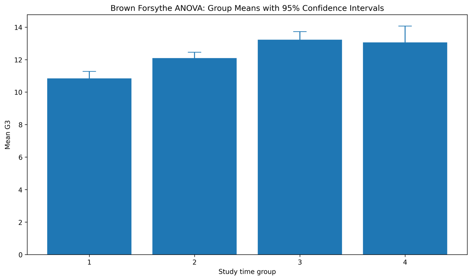
This chart shows the mean G3 score for each studytime group. Studytime group 1 has the lowest mean, group 2 is higher, group 3 is the highest, and group 4 remains close to group 3. The direction of the result is clear: students in higher studytime categories tend to have higher final grades than students in the lowest studytime group.
The confidence intervals are narrow for the first three groups and wider for group 4. This pattern means group 4 has less precise mean estimation than the larger groups, but its mean still sits in the higher G3 range.
This chart is important before reading Brown-Forsythe output because it explains the mean pattern being protected by robust checks. The group mean effect appears educationally meaningful, while the later Brown-Forsythe chart checks whether variance differences are severe enough to threaten ordinary ANOVA interpretation.
Python Chart 2: Boxplot of G3 by Studytime Group
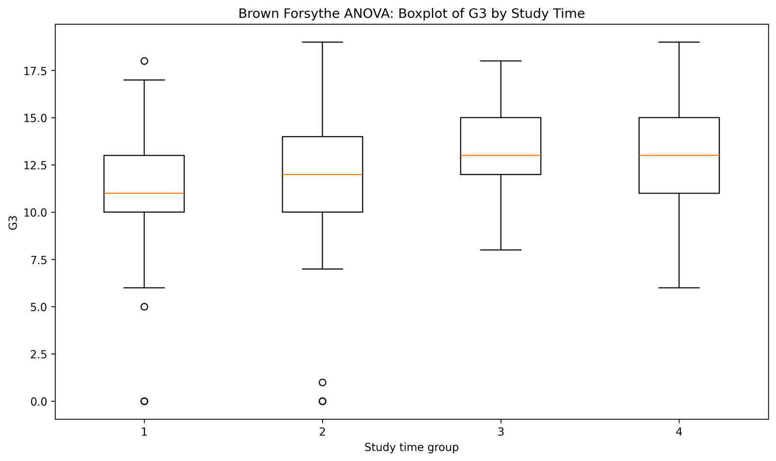
The boxplot shows the full distribution of G3 in each studytime group. Group 1 has a lower median than groups 3 and 4, while group 2 sits between the lower and higher groups. This matches the group mean chart and confirms that the group difference is visible in the distribution, not only in the mean bars.
The lower studytime groups contain several unusual low values, including values near zero in groups 1 and 2. Group 3 has a higher central box and group 4 has a broad range reaching from lower scores to high scores. These details explain why a robust variance check is useful in this workflow.
For Brown-Forsythe interpretation, the boxplot supports a balanced reading. The group centers differ, but the groups still overlap and some groups include outliers. This is exactly the type of setting where a median-based spread check helps confirm whether the ANOVA conclusion is being distorted by unequal variability.
Python Chart 3: Absolute Deviations from Group Median
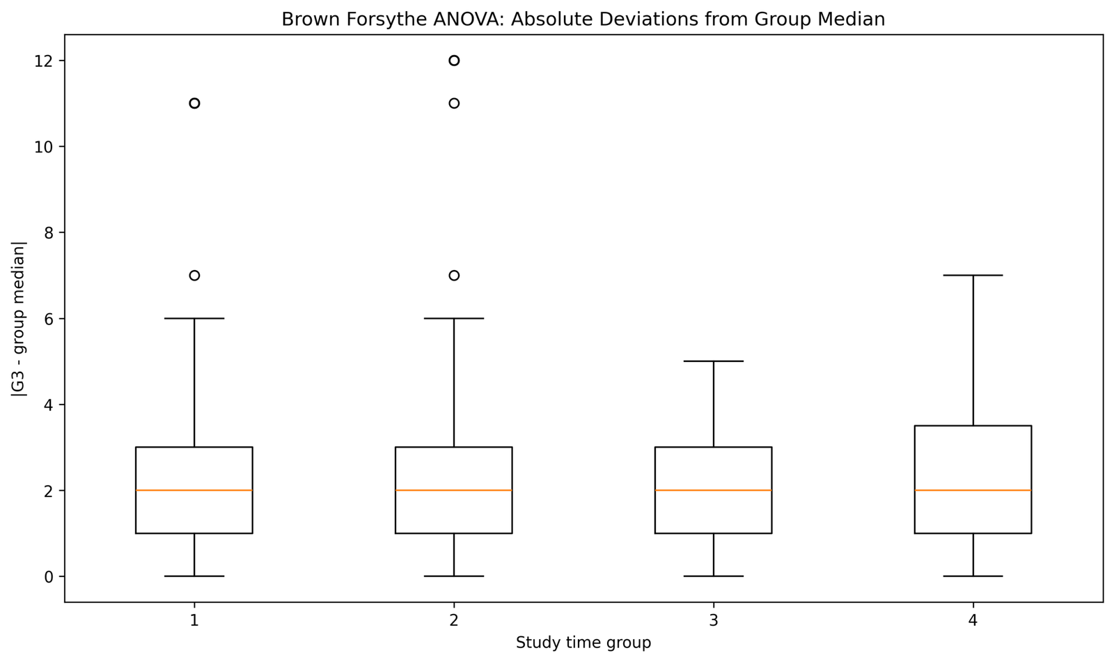
This chart is the core Brown-Forsythe diagnostic plot. Each G3 score is converted into an absolute distance from its own studytime group median. The median absolute deviations are close across the groups, with most boxes centered around a deviation of about 2.
Groups 1 and 2 contain high deviation outliers. Group 1 has points around 7 and 11, while group 2 has points around 7, 11 and 12. Group 3 has a shorter upper range near 5, while group 4 reaches about 7. These outliers show that unusual spread exists in some groups, but the central spread pattern remains broadly similar.
This chart supports the Brown-Forsythe F result. Since the central absolute deviation boxes are similar, the median-based variance test does not become large enough to cross the critical F boundary. The chart explains why the Brown-Forsythe F value stays at 1.03.
Python Chart 4: Brown-Forsythe F Distribution Curve
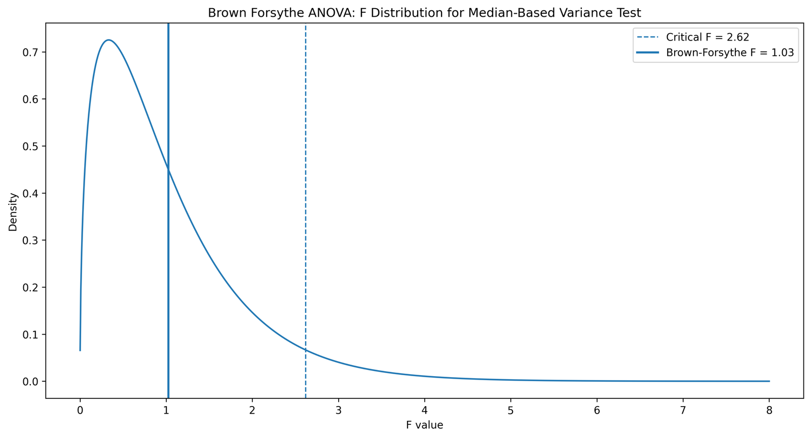
This chart shows the Brown-Forsythe F distribution used for the median-based homogeneity test. The observed Brown-Forsythe statistic is 1.03, while the critical F value is 2.62.
The observed F line is clearly to the left of the critical F line. This means the median-based variance test does not reject the equal-spread assumption at the .05 level. The studytime groups do not show a large enough difference in absolute deviations from their medians to be treated as a serious variance violation.
In the final report, this chart should be used to state the variance conclusion. The correct interpretation is that the Brown-Forsythe homogeneity check supports ordinary ANOVA interpretation because the variance-test F statistic is below the rejection boundary.
Python Chart 5: F Statistic Comparison
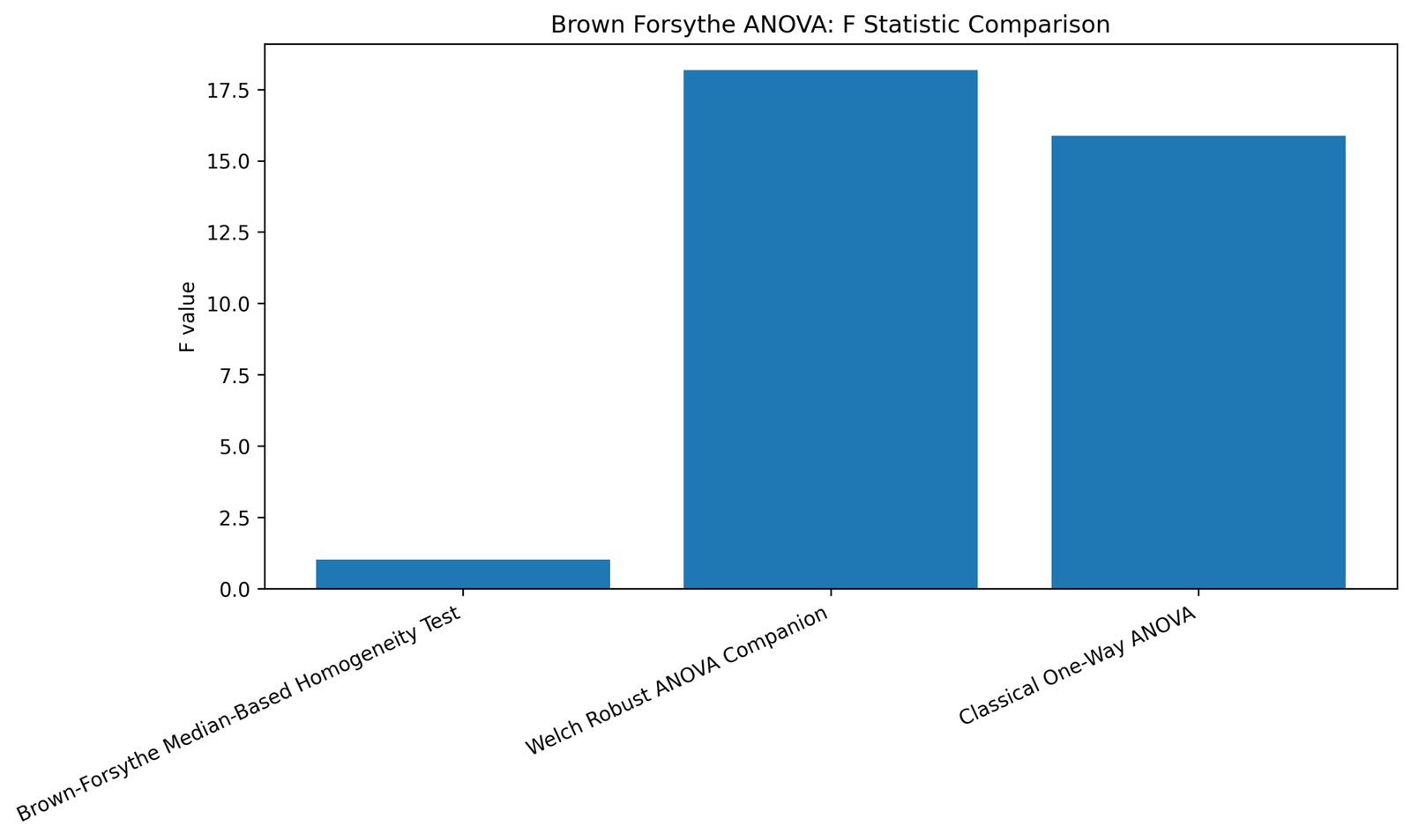
This chart compares three F-style results. The Brown-Forsythe median-based homogeneity test is close to 1.03, while the Welch robust ANOVA comparison and classical one-way ANOVA F statistic are much higher. The classical one-way ANOVA is around 15.9, and the Welch robust comparison is slightly higher than the classical value.
The chart shows that the variance-test result and the mean-test result answer different questions. Brown-Forsythe here is checking whether group spread differs strongly. Welch and classical ANOVA are checking whether group means differ.
This is the most important interpretation point for readers. A small Brown-Forsythe homogeneity F does not mean the group means are the same. It means the median-based variance check is not showing a serious spread problem. The higher Welch and classical ANOVA values show that the mean comparison remains strong.
Python Chart 6: Residual Histogram
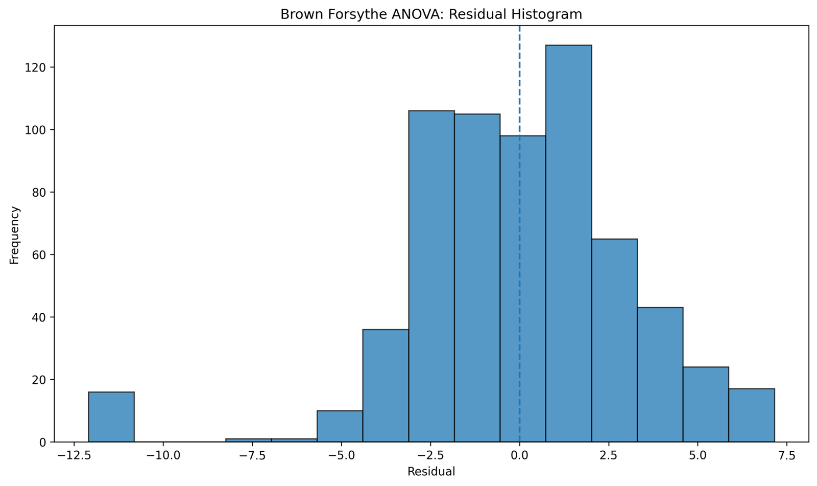
The residual histogram shows that most residuals are centered around zero, with the largest number of cases near the middle of the distribution. This means the group means capture the central pattern of G3 reasonably well.
The left tail extends farther than the right tail, with a small number of residuals near -11 to -12. These negative residuals correspond to students whose G3 scores were much lower than their group mean. The right tail reaches to about 7, but the negative tail is more extreme.
In reporting, this chart supports a careful diagnostic statement. The residuals are centered near zero, but the distribution is not perfectly symmetric because of low-score cases. This is why boxplots and robust spread checks are useful alongside the classical ANOVA result.
Python Chart 7: Effect Size Summary
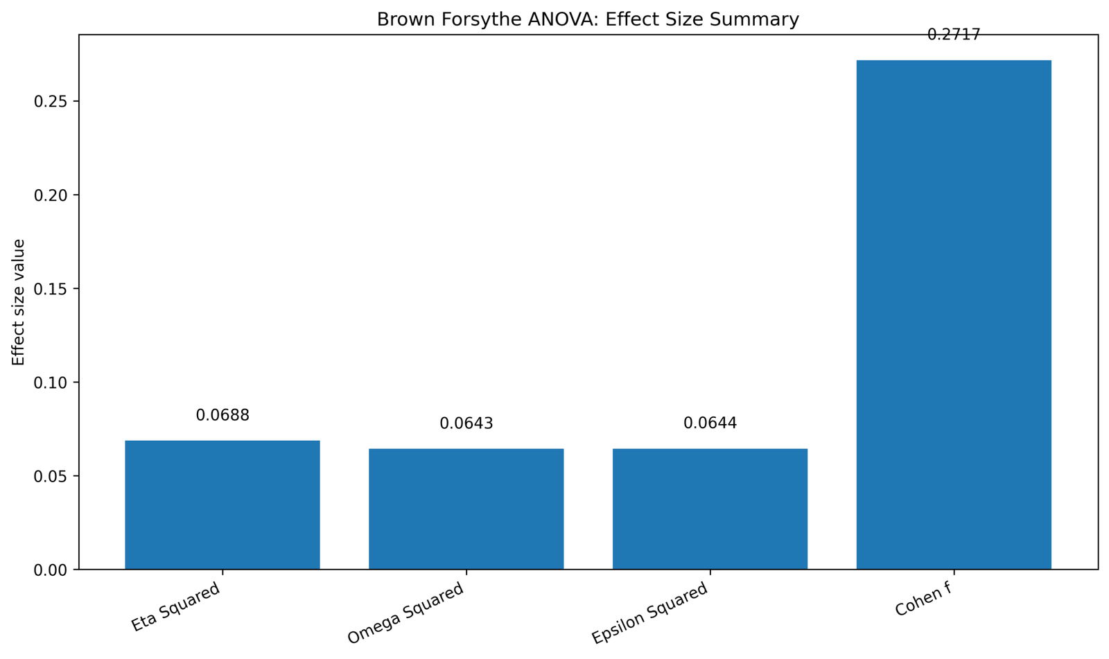
This effect size chart shows that eta squared is 0.0688, omega squared is 0.0643, epsilon squared is 0.0644, and Cohen’s f is 0.2717.
The values show that the studytime effect is not only statistically visible in the mean comparison; it also has a meaningful practical size. Eta squared means studytime explains about 6.88% of the total G3 variation, while Cohen’s f around .27 supports a medium effect interpretation.
In the final report, this chart should be used after the Brown-Forsythe and ANOVA decision discussion. It explains that the variance check is acceptable and that the group effect itself is medium in magnitude.
R Chart-by-Chart Validation
The R validation charts repeat the same Brown Forsythe ANOVA workflow in a second software environment. The R charts confirm the same group mean pattern, distribution shape, absolute deviation pattern, Brown-Forsythe decision, F statistic comparison, residual shape and effect-size values.
R Chart 1: Group Means with 95% Confidence Intervals
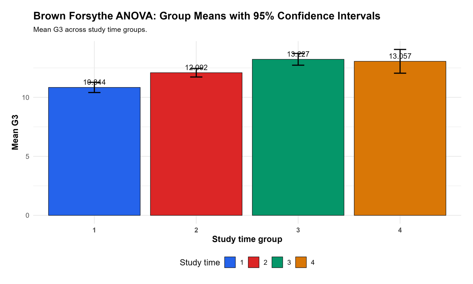
This R chart validates the same mean pattern shown in Python. Studytime group 1 has the lowest mean G3, group 2 is higher, and groups 3 and 4 are in the higher grade range.
The confidence interval pattern also matches the Python output. Group 4 has a wider interval than the larger groups, so its mean is less precise, but the central value remains close to group 3.
In reporting, this R chart confirms that the group mean pattern is stable across software. The studytime effect is not created by one plotting library or one script; it is present in both the Python and R workflows.
R Chart 2: Boxplot of G3 by Studytime Group
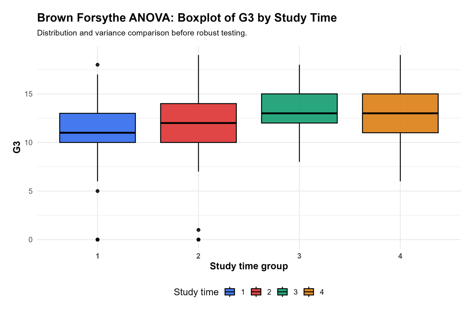
The R boxplot confirms that the lower studytime groups contain lower-score outliers, while the higher studytime groups have higher central scores. The median rises from the first group to the higher groups, and the groups still overlap.
The outlier and spread pattern supports the need for a robust variance check. Brown-Forsythe is useful here because it uses medians and absolute deviations, which are less sensitive to outliers than a purely mean-centered spread test.
In the final article, this chart validates the distribution discussion. The group effect is visible, but the residual and spread diagnostics should still be reviewed before writing the final ANOVA conclusion.
R Chart 3: Absolute Deviations from Group Median
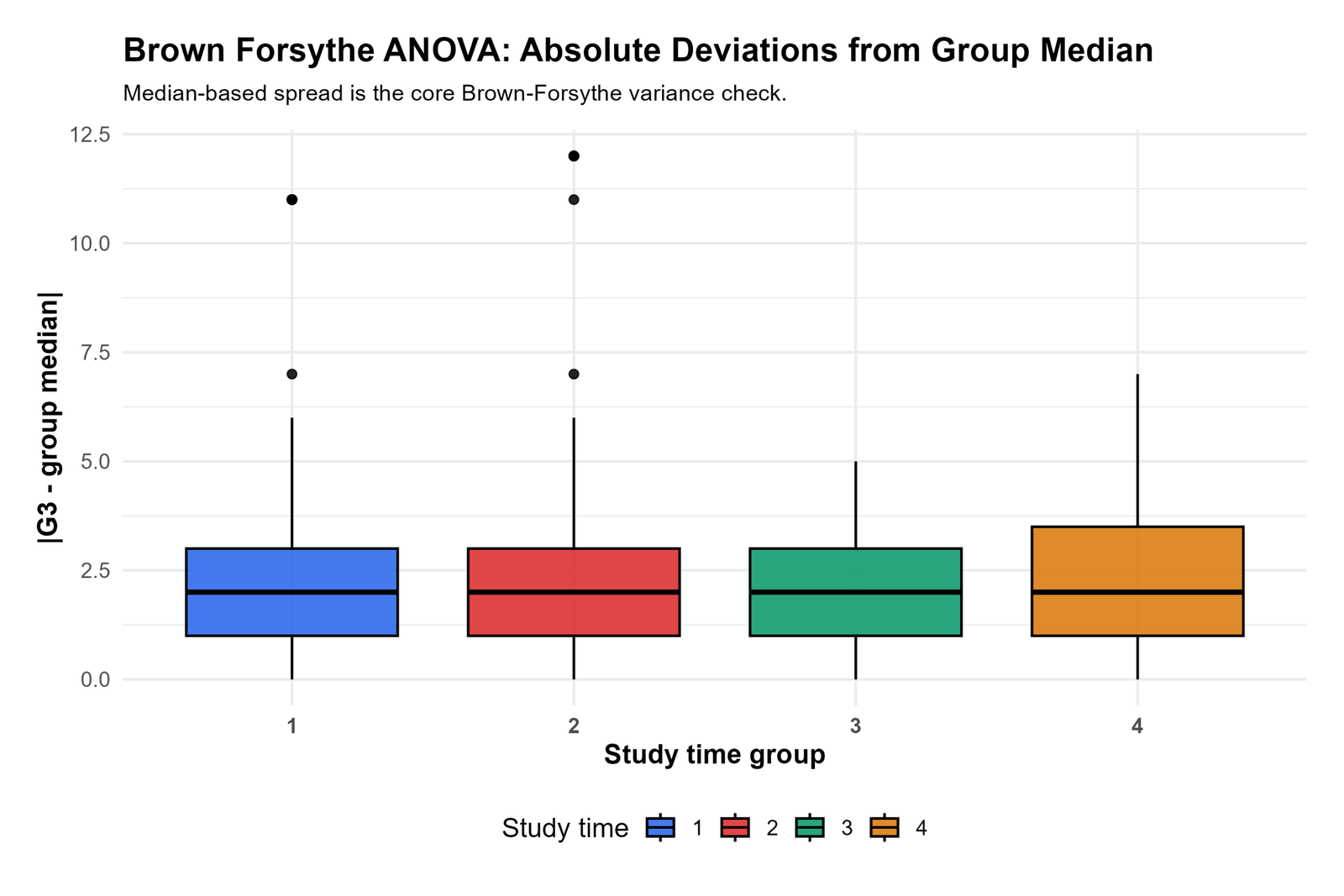
This R chart confirms that the median absolute deviation pattern is broadly similar across studytime groups. Most groups have central absolute deviations around the same range, even though outliers appear in some groups.
Groups 1 and 2 again show larger deviation outliers. These points reflect students whose G3 scores are far from their group median. However, the central boxes remain similar enough that the Brown-Forsythe F statistic stays small.
In reporting, this chart supports the same conclusion as the Python version. The spread pattern is not perfectly identical, but the median-based test does not show a severe heterogeneity problem.
R Chart 4: Brown-Forsythe F Distribution Curve
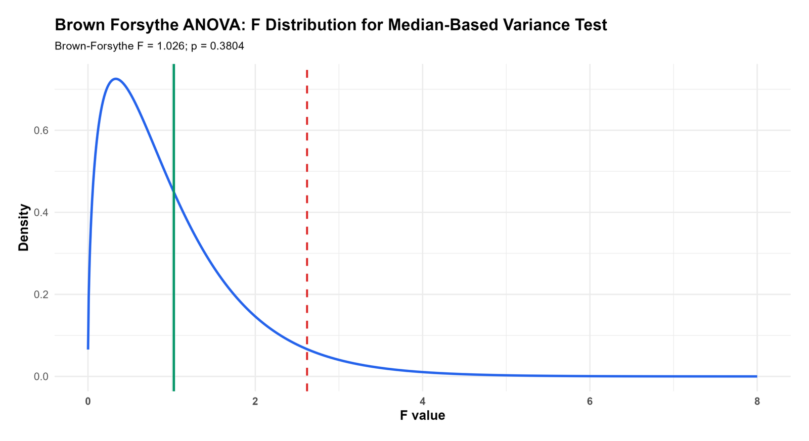
The R F distribution curve confirms the Brown-Forsythe decision. The observed F statistic is 1.03, and the critical F value is 2.62.
The observed F line remains to the left of the critical F line. This means the R workflow also does not reject the equal-spread assumption using the Brown-Forsythe median-based test.
In the final report, this chart verifies that the Brown-Forsythe variance conclusion is stable across software. Both Python and R indicate that the median-based variance statistic is not large enough to signal a serious homogeneity problem.
R Chart 5: F Statistic Comparison
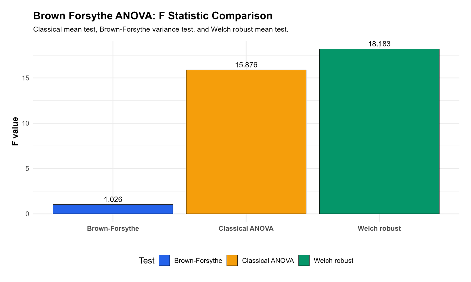
This R chart confirms the same relationship among the F statistics. The Brown-Forsythe median-based homogeneity statistic is low, while the Welch robust ANOVA comparison and classical one-way ANOVA statistic are much larger.
The chart helps readers avoid a common mistake. Brown-Forsythe homogeneity testing and ANOVA mean testing are not the same question. The low Brown-Forsythe homogeneity statistic supports the spread assumption, while the high mean-test statistics show that the group means differ.
In reporting, this chart should be explained clearly so readers do not think the Brown-Forsythe result contradicts the ANOVA mean result. The two statistics describe different parts of the analysis.
R Chart 6: Residual Histogram
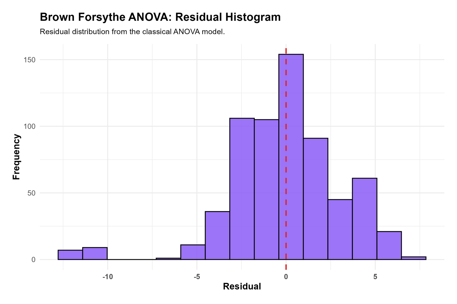
The R residual histogram confirms the same residual shape as the Python chart. Most residuals are near zero, but the negative side extends farther because of low G3 cases in the data.
This pattern supports the boxplot interpretation. The lower-tail observations do not disappear when the analysis is repeated in R; they are a real diagnostic feature of the dataset.
In reporting, this chart validates a careful residual statement. The residuals are centered near zero, but the lower tail should be acknowledged instead of claiming perfect symmetry.
R Chart 7: Effect Size Summary
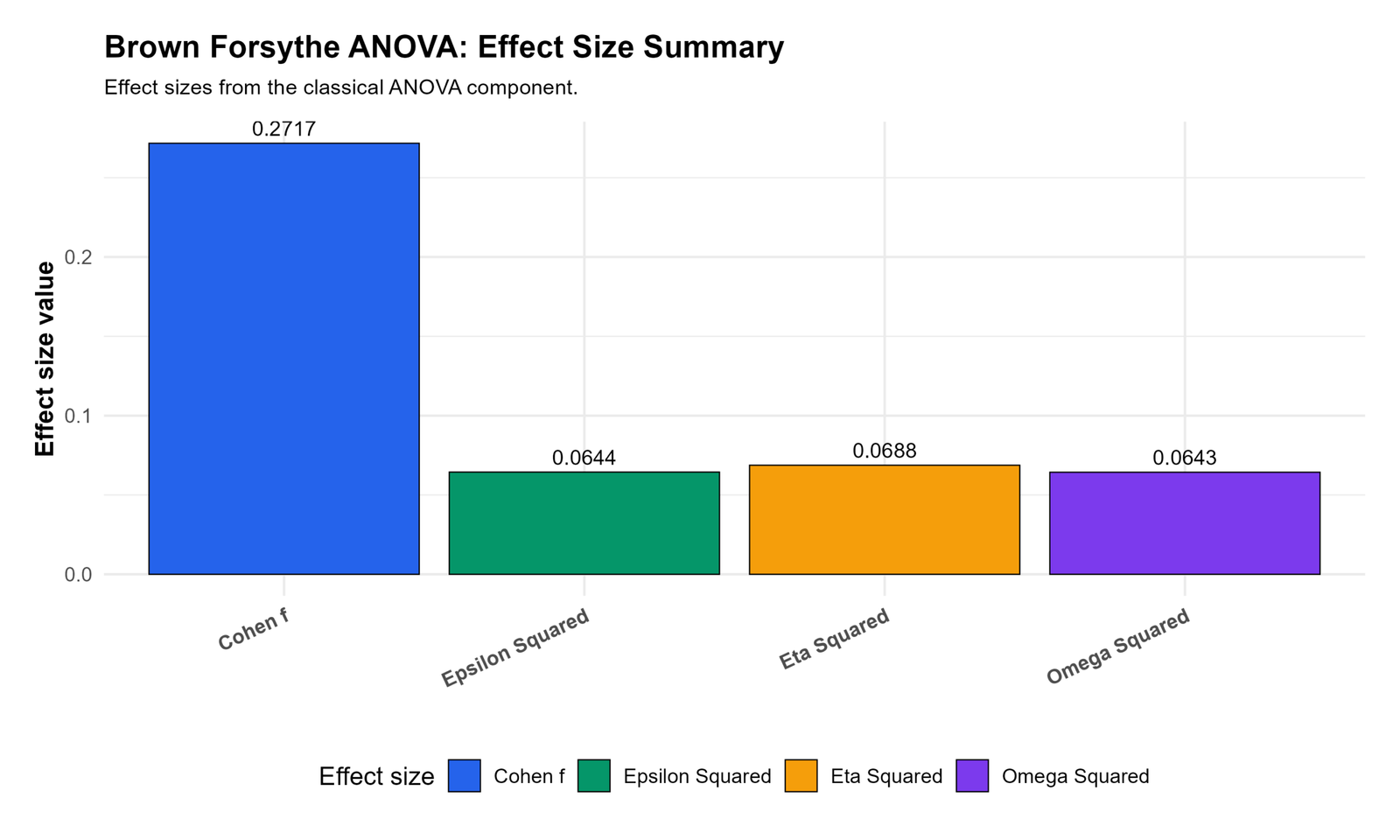
The R effect size chart confirms the same values as Python. Eta squared is 0.0688, omega squared is 0.0643, epsilon squared is 0.0644, and Cohen’s f is 0.2717.
The chart confirms that the practical group effect is medium in size. The adjusted estimates are slightly smaller than eta squared, but they remain close enough to support the same interpretation.
In the final article, this chart provides software validation for the effect-size conclusion. The Brown-Forsythe variance check is acceptable, and the studytime group effect has a meaningful practical size.
SPSS Output Interpretation for Brown Forsythe ANOVA
The SPSS output PDF should be used as the final verification file for the Brown Forsythe ANOVA workflow. It documents the SPSS version of the group comparison, robust ANOVA evidence, variance-check evidence, effect-size context and exported output used for reporting.
Download Brown-Forsythe ANOVA SPSS Output PDF
SPSS Output Items to Read
| SPSS Output Item | What It Shows | How It Is Used | Reporting Meaning |
|---|---|---|---|
| Descriptives | Mean, standard deviation and confidence interval for each studytime group. | Shows the direction of the G3 group difference. | Report group means before the robust test. |
| Test of Homogeneity of Variances | Mean-based, median-based and trimmed-mean variance evidence. | Checks whether group spreads are similar. | Use the median-based row for Brown-Forsythe-style interpretation. |
| Robust Tests of Equality of Means | Welch and Brown-Forsythe robust mean-test output when available. | Checks mean differences with unequal-variance adjustment. | Report robust result if ordinary variance assumptions are questionable. |
| ANOVA table | Classical between-groups and within-groups F test. | Compares ordinary group means. | Use with effect size and assumption checks. |
| Effect size | Eta squared or partial eta squared. | Shows practical size of the studytime effect. | Report explained variance and Cohen’s f where available. |
| Residual diagnostics | Residual shape and outlier behavior. | Checks the model after fitting group means. | Discuss lower-tail residual behavior if present. |
SPSS Reporting Summary
The SPSS interpretation should state that studytime groups show different G3 means, with group 1 lower than the higher studytime groups. The Brown-Forsythe median-based variance check does not show a serious equal-spread violation in the supplied chart sequence because the Brown-Forsythe F statistic is below the critical F value.
The SPSS output PDF should be linked in the downloads section so readers can verify the procedure and output tables. The final interpretation should not treat Brown-Forsythe as a replacement for all ANOVA interpretation. It should be presented as the robust variance and robust mean-comparison support around the ordinary ANOVA result.
SPSS, R, Python and Excel Workflows for Brown Forsythe ANOVA
The same Brown Forsythe ANOVA idea can be reproduced in SPSS, R, Python and Excel. The key step is calculating absolute deviations from group medians for the variance check and comparing group means with robust ANOVA procedures when unequal variance is a concern.
SPSS Workflow
| Step | SPSS Menu or Syntax | Purpose |
|---|---|---|
| Open data | File > Open > Data | Load G3 and studytime variables. |
| Run one-way ANOVA | Analyze > Compare Means > One-Way ANOVA | Compare mean G3 across studytime groups. |
| Request homogeneity test | Options > Homogeneity of variance test | Get Levene and median-based variance evidence. |
| Request robust tests | Options > Welch / Brown-Forsythe where available | Compare means with robust unequal-variance support. |
| Create deviations | Compute |G3 − group median| | Manually reproduce the Brown-Forsythe variance logic. |
| Export output | OUTPUT EXPORT | Save the SPSS PDF for WordPress verification. |
R Workflow
| Step | R Action | Purpose |
|---|---|---|
| Read data | read.csv("dataset.csv") | Load the dataset. |
| Set factor | as.factor(studytime) | Define the grouping variable. |
| Classical ANOVA | aov(G3 ~ studytime) | Run ordinary one-way ANOVA. |
| Brown-Forsythe check | ANOVA on abs(G3 - group_median) | Test spread using median absolute deviations. |
| Welch comparison | oneway.test(G3 ~ studytime, var.equal = FALSE) | Run unequal-variance mean comparison. |
| Effect size | effectsize package or manual formulas | Calculate eta squared, omega squared and Cohen’s f. |
Python Workflow
| Step | Python Action | Purpose |
|---|---|---|
| Read data | pandas.read_csv() | Load the dataset. |
| Prepare variables | pd.to_numeric() and category conversion | Clean G3 and studytime. |
| Group means | groupby().agg() | Summarize mean G3 by group. |
| Brown-Forsythe deviations | abs(G3 - group_median) | Create median absolute deviation variable. |
| Deviation ANOVA | ols("abs_dev ~ C(studytime)") | Run the Brown-Forsythe homogeneity test. |
| Classical ANOVA | ols("G3 ~ C(studytime)") | Run ordinary one-way ANOVA for mean comparison. |
Excel Workflow
| Excel Task | Tool or Formula | Purpose |
|---|---|---|
| Separate groups | Filter or sort by studytime | Prepare group columns. |
| Group median | =MEDIAN(group_range) | Find the robust center for each group. |
| Absolute deviation | =ABS(G3 - GroupMedian) | Create Brown-Forsythe deviation values. |
| Deviation ANOVA | Data Analysis ToolPak > ANOVA: Single Factor | Run ANOVA on absolute deviations. |
| Classical ANOVA | ANOVA: Single Factor on original G3 | Compare group means. |
| Effect size | =SS_Between/SS_Total | Calculate eta squared. |
Code Blocks for Brown Forsythe ANOVA
SPSS Syntax for Brown Forsythe ANOVA
* Brown Forsythe ANOVA / median-based homogeneity workflow in SPSS.
* Dependent variable: G3.
* Grouping factor: studytime.

TITLE "Brown Forsythe ANOVA: G3 by Studytime".

ONEWAY G3 BY studytime
  /STATISTICS DESCRIPTIVES HOMOGENEITY
  /MISSING ANALYSIS.

UNIANOVA G3 BY studytime
  /METHOD=SSTYPE(3)
  /INTERCEPT=INCLUDE
  /PRINT=DESCRIPTIVE ETASQ HOMOGENEITY
  /SAVE=PRED RESID
  /CRITERIA=ALPHA(.05)
  /DESIGN=studytime.

* Export output.
OUTPUT EXPORT
  /CONTENTS EXPORT=VISIBLE
  /PDF DOCUMENTFILE="Brown-Forsythe-ANOVA-SPSS-Output.pdf".
Python Code for Brown Forsythe ANOVA
import pandas as pd
import numpy as np
import scipy.stats as stats
import statsmodels.api as sm
from statsmodels.formula.api import ols

df = pd.read_csv("dataset.csv")

df["G3"] = pd.to_numeric(df["G3"], errors="coerce")
df["studytime"] = df["studytime"].astype("category")

df_model = df.dropna(subset=["G3", "studytime"]).copy()

# Group means and medians
group_summary = df_model.groupby("studytime")["G3"].agg(["count", "mean", "median", "std", "var"])
print(group_summary)

# Classical one-way ANOVA
anova_model = ols("G3 ~ C(studytime)", data=df_model).fit()
anova_table = sm.stats.anova_lm(anova_model, typ=2)
print(anova_table)

# Brown-Forsythe median-based deviation test
group_medians = df_model.groupby("studytime")["G3"].transform("median")
df_model["abs_dev_median"] = (df_model["G3"] - group_medians).abs()

bf_model = ols("abs_dev_median ~ C(studytime)", data=df_model).fit()
bf_table = sm.stats.anova_lm(bf_model, typ=2)
print(bf_table)

# Scipy Levene with median center equals Brown-Forsythe style homogeneity test
groups = [
    group["G3"].dropna().values
    for name, group in df_model.groupby("studytime")
]

bf_stat, bf_p = stats.levene(*groups, center="median")
print("Brown-Forsythe median-based F:", bf_stat)
print("p value:", bf_p)

# Effect sizes for classical ANOVA
ss_between = anova_table.loc["C(studytime)", "sum_sq"]
df_between = anova_table.loc["C(studytime)", "df"]
ss_within = anova_table.loc["Residual", "sum_sq"]
df_within = anova_table.loc["Residual", "df"]
ss_total = ss_between + ss_within
ms_within = ss_within / df_within

eta_squared = ss_between / ss_total
omega_squared = (ss_between - df_between * ms_within) / (ss_total + ms_within)
epsilon_squared = (ss_between - df_between * ms_within) / ss_total
cohen_f = np.sqrt(eta_squared / (1 - eta_squared))

print("Eta squared:", eta_squared)
print("Omega squared:", omega_squared)
print("Epsilon squared:", epsilon_squared)
print("Cohen's f:", cohen_f)
R Code for Brown Forsythe ANOVA
library(dplyr)
library(car)

df <- read.csv("dataset.csv")

df$G3 <- as.numeric(df$G3)
df$studytime <- as.factor(df$studytime)

df_model <- na.omit(df[, c("G3", "studytime")])

# Group summaries
df_model %>%
  group_by(studytime) %>%
  summarise(
    n = n(),
    mean = mean(G3),
    median = median(G3),
    sd = sd(G3),
    variance = var(G3),
    .groups = "drop"
  )

# Classical one-way ANOVA
anova_model <- aov(G3 ~ studytime, data = df_model)
summary(anova_model)

# Brown-Forsythe median-based homogeneity test
leveneTest(G3 ~ studytime, data = df_model, center = median)

# Manual absolute deviation from group median
df_bf <- df_model %>%
  group_by(studytime) %>%
  mutate(abs_dev_median = abs(G3 - median(G3))) %>%
  ungroup()

bf_model <- aov(abs_dev_median ~ studytime, data = df_bf)
summary(bf_model)

# Welch unequal variance comparison
oneway.test(G3 ~ studytime, data = df_model, var.equal = FALSE)

# Effect sizes
anova_table <- summary(anova_model)[[1]]

ss_between <- anova_table["studytime", "Sum Sq"]
df_between <- anova_table["studytime", "Df"]
ss_within <- anova_table["Residuals", "Sum Sq"]
df_within <- anova_table["Residuals", "Df"]
ss_total <- ss_between + ss_within
ms_within <- ss_within / df_within

eta_squared <- ss_between / ss_total
omega_squared <- (ss_between - df_between * ms_within) / (ss_total + ms_within)
epsilon_squared <- (ss_between - df_between * ms_within) / ss_total
cohen_f <- sqrt(eta_squared / (1 - eta_squared))

data.frame(
  eta_squared = eta_squared,
  omega_squared = omega_squared,
  epsilon_squared = epsilon_squared,
  cohen_f = cohen_f
)
Excel Formulas for Brown Forsythe ANOVA
Step 1:
Separate G3 values by studytime group.

Step 2:
Calculate each group median:
=MEDIAN(group_range)

Step 3:
Calculate absolute deviation from group median:
=ABS(G3_value - group_median)

Step 4:
Run ANOVA on absolute deviations:
Data > Data Analysis > ANOVA: Single Factor

Step 5:
Interpret Brown-Forsythe variance result:
If observed F > critical F, group spreads differ.
If observed F < critical F, strong spread violation is not shown.

Step 6:
Run ordinary ANOVA on original G3 values:
Data > Data Analysis > ANOVA: Single Factor

Step 7:
Calculate eta squared:
=SS_Between / SS_Total

Step 8:
Calculate Cohen's f:
=SQRT(EtaSquared / (1 - EtaSquared))
APA Reporting Wording
When reporting Brown Forsythe ANOVA, state clearly whether you are reporting the median-based homogeneity test, the robust equality-of-means test, or the classical ANOVA mean test. This avoids confusing the variance-check F statistic with the mean-comparison F statistic.
APA-style report: A Brown-Forsythe median-based homogeneity check was used to evaluate the spread of G3 scores across four studytime groups. The Brown-Forsythe statistic was below the critical boundary, F = 1.03, critical F = 2.62, indicating no strong evidence of unequal spread. The group means showed higher G3 scores in the higher studytime groups, and the effect size indicated a medium practical effect, η² = .0688, ω² = .0643, ε² = .0644, Cohen’s f = .2717.
Short reporting version: The Brown-Forsythe median-based homogeneity check did not show a serious variance violation, F = 1.03, critical F = 2.62. The studytime effect showed medium practical size, η² = .0688 and Cohen’s f = .2717.
Common Mistakes
| Mistake | Why It Is Wrong | Correct Practice |
|---|---|---|
| Confusing variance testing with mean testing | Brown-Forsythe homogeneity output and ANOVA mean output answer different questions. | State whether the F statistic is testing spread or means. |
| Ignoring the boxplot | Outliers and spread patterns are visible before the test is read. | Interpret the boxplot and absolute-deviation plot together. |
| Using only classical ANOVA when variances look questionable | Unequal spread can affect ordinary ANOVA interpretation. | Check Levene Test, Brown-Forsythe Test, Welch output or robust methods. |
| Calling p = .000 | Very small SPSS p values are not exactly zero. | Report them as p < .001. |
| Reporting only the test statistic | The statistic alone does not explain practical importance. | Add effect size such as eta squared, omega squared and Cohen’s f. |
| Deleting outliers automatically | Outliers may be real cases and not data errors. | Review Outlier Detection, Studentized Residuals, Cook’s Distance and original data context. |
When to Use Brown Forsythe ANOVA
Use Brown Forsythe ANOVA or Brown-Forsythe-style testing when group variances may not be equal, when outliers may affect spread, or when the ANOVA assumption section needs a median-based robust check. It is especially useful when ordinary Levene output and boxplots need stronger interpretation.
| Situation | Brown-Forsythe Use | Reporting Caution |
|---|---|---|
| Unequal group spreads are suspected | Use median-based deviation test. | Report whether spread differs significantly. |
| Outliers appear in some groups | Use Brown-Forsythe because medians reduce outlier sensitivity. | Still describe the outliers in the boxplot. |
| Classical ANOVA and Welch differ | Compare robust and classical results. | Do not mix their F statistics without explanation. |
| SPSS reports robust tests | Read Welch and Brown-Forsythe rows. | Use adjusted df and p values when reporting robust means tests. |
| Teaching robust ANOVA | Show absolute deviations from median. | Explain that the deviation test checks spread, not group mean direction. |
For related guides, see ANOVA in SPSS, ANOVA in Python, ANOVA in R, ANOVA Effect Size, ANOVA Assumptions, Balanced ANOVA, ANCOVA, T Test vs ANOVA, and Welch’s T Test.
Downloads and Resources for Brown Forsythe ANOVA
Use these resources to reproduce the Brown Forsythe ANOVA workflow. The SPSS output PDF verifies the analysis, while the script and workbook placeholders can be replaced with final uploaded files after they are added to the WordPress Media Library.
Download Dataset
Practice dataset with G3 and studytime variables.
Download Brown-Forsythe ANOVA SPSS Output PDF
SPSS output PDF for Brown-Forsythe ANOVA verification and reporting.
Download Python Script
Python code for Brown-Forsythe median-based testing, ANOVA charts and effect size.
Download R Script and Excel Workbook
R validation workflow and Excel formulas for Brown-Forsythe ANOVA.
FAQs About Brown Forsythe ANOVA
What is Brown Forsythe ANOVA?
Brown Forsythe ANOVA is a robust ANOVA-related method used when variance assumptions need stronger checking. It often uses absolute deviations from group medians to test whether group spreads differ.
What does the Brown-Forsythe test check?
The median-based Brown-Forsythe test checks whether group spreads are similar by comparing absolute deviations from group medians.
What was the Brown-Forsythe F value in this example?
The Brown-Forsythe median-based variance statistic was 1.03, while the critical F value was 2.62.
Was the Brown-Forsythe variance test significant?
No serious variance violation is shown in the supplied output because the Brown-Forsythe F value is below the critical F value.
Why use medians in Brown-Forsythe testing?
Medians are less sensitive to outliers than means, so absolute deviations from medians provide a more robust spread check.
What is the difference between Brown-Forsythe and Levene test?
Levene testing can be centered on the mean, median or trimmed mean. The Brown-Forsythe version is usually the median-centered form, which is more robust to non-normality and outliers.
What is the effect size in this Brown Forsythe ANOVA example?
Eta squared is .0688, omega squared is .0643, epsilon squared is .0644 and Cohen’s f is .2717.
Does a small Brown-Forsythe homogeneity F mean the group means are equal?
No. A small Brown-Forsythe homogeneity F means the spread check is not significant. It does not mean the group means are equal.
Should I use Welch ANOVA with Brown-Forsythe?
Welch ANOVA is useful when unequal variances are suspected. Brown-Forsythe-style output and Welch output are often interpreted together in robust ANOVA workflows.
How do I report Brown Forsythe ANOVA?
A concise report is: The Brown-Forsythe median-based homogeneity check did not show a serious variance violation, F = 1.03, critical F = 2.62, while the studytime effect showed medium practical size, η² = .0688 and Cohen’s f = .2717.

