
Regression Assumption, Multicollinearity, VIF and Tolerance
Variance Inflation Factor: Formula, Interpretation, SPSS, Python, R and Excel Guide
Variance Inflation Factor, usually written as VIF, is a regression diagnostic used to detect multicollinearity among predictors. A high VIF means that a predictor is strongly explained by other predictors, which can inflate the variance of regression coefficients and make coefficient signs, standard errors, and p-values unstable. This guide explains Variance Inflation Factor with verified SPSS output, Python charts, R validation charts, Excel workflow, interpretation rules, code blocks, APA wording, common mistakes, and downloadable resources.
Quick Answer: Variance Inflation Factor Result
The verified regression model predicted G3 final grade from 13 predictors: G1, G2, studytime, failures, absences, age, Medu, Fedu, traveltime, famrel, freetime, goout and health. The model was strong overall, with R = .923, R² = .852, adjusted R² = .849, F(13, 635) = 281.518, and p < .001. The main VIF result is that all predictors stayed below the common moderate-risk threshold of VIF = 5. The highest VIF was for G2 = 4.204, followed by G1 = 4.195. Both are elevated but still acceptable under the common VIF ≤ 5 rule.
Hypothesis-style decision: The null assumption says the regression model does not have harmful multicollinearity, meaning H0: VIF ≤ 5 and tolerance ≥ .20 for all predictors. The alternative assumption says at least one predictor has problematic multicollinearity, meaning H1: VIF > 5 or tolerance < .20 for at least one predictor. Since the highest VIF is 4.204 and the lowest tolerance is .238, the VIF-based decision is to retain the null assumption of acceptable multicollinearity. However, G1 and G2 should still be watched because their correlation is very strong and they are the closest predictors to the threshold.
Final interpretation: Variance Inflation Factor analysis showed no serious multicollinearity under the common VIF > 5 or VIF > 10 rules. All predictors were in the acceptable VIF range. The only predictors requiring attention were G1 and G2, because their VIF values were about 4.20 and their tolerance values were about .238. The regression model can be reported, but G1 and G2 should be interpreted carefully because they are strongly correlated grade predictors.
Important note: VIF is not a normality test, and it does not test residual shape. It checks predictor multicollinearity in regression. For normality-related diagnostics, use tools such as the Q-Q plot normality check, P-P plot normality check, Kolmogorov-Smirnov test, Lilliefors test, and D’Agostino-Pearson test.
Table of Contents
- What Is Variance Inflation Factor?
- VIF Formula and Tolerance Formula
- Null and Alternative Hypothesis for VIF
- Dataset and Regression Variables Used
- Verified SPSS Output Interpretation
- Python Chart-by-Chart Interpretation
- R Chart-by-Chart Validation
- SPSS, R, Python and Excel Workflows
- Code Blocks for VIF
- APA Reporting Wording
- Common Mistakes
- When to Use Variance Inflation Factor
- Downloads and Resources
- Related Guides
- FAQs
What Is Variance Inflation Factor?
Variance Inflation Factor measures how much the variance of a regression coefficient is inflated because a predictor is correlated with other predictors in the same model. When predictors overlap strongly, the model can still predict the outcome well, but individual coefficients may become unstable. This means the sign, size, standard error, and significance of a coefficient can change when correlated predictors are added or removed.
In simple words, VIF answers this question: “How much is this predictor’s coefficient variance inflated because the predictor shares information with other predictors?” A VIF close to 1 means the predictor is mostly independent of the other predictors. A VIF around 2 to 4 shows some overlap but usually not severe. A VIF above 5 is often treated as a warning. A VIF above 10 is commonly treated as serious multicollinearity.
This guide uses a regression model predicting G3 final grade. The predictors include previous grades, study time, failures, absences, age, parental education variables, travel time, family relationship, free time, going out, and health. Because G1 and G2 are previous grade variables, they are naturally correlated. The VIF output confirms this: G1 and G2 have the highest VIF values, but they still remain below 5.
Practical meaning: VIF does not tell whether the model predicts well. The model can have a high R² and still have multicollinearity problems. VIF tells whether individual predictor coefficients are likely to be inflated, unstable, or difficult to interpret because predictors overlap with each other.
VIF Formula and Tolerance Formula
The Variance Inflation Factor for a predictor is based on how well that predictor can be predicted from all other predictors. The formula is:
Here, R²j is the R-squared value from an auxiliary regression where predictor Xj is predicted by all the other predictors. If the other predictors explain a large amount of Xj, then R²j is high and VIF becomes high.
Tolerance is the inverse of VIF:
So a high VIF means low tolerance. A low tolerance means the predictor has little unique variance left after accounting for the other predictors.
| VIF / Tolerance Rule | Common Interpretation | Action |
|---|---|---|
| VIF ≈ 1 | No meaningful multicollinearity. | Safe to interpret coefficient normally. |
| VIF 1 to 3 | Low to mild predictor overlap. | Usually acceptable. |
| VIF 3 to 5 | Elevated but often acceptable. | Interpret with caution and inspect correlations. |
| VIF 5 to 10 | Moderate multicollinearity warning. | Consider removing, combining, or rethinking predictors. |
| VIF > 10 | Serious multicollinearity. | Model revision is usually needed. |
| Tolerance < .20 | Common warning threshold. | Review predictor overlap. |
| Tolerance < .10 | Serious multicollinearity threshold. | Strong model revision warning. |
Threshold caution: VIF thresholds are guidelines, not absolute laws. Some fields use VIF > 5 as the main warning rule, while others use VIF > 10. For student-friendly reporting, this guide uses VIF ≤ 5 as acceptable, VIF 5–10 as moderate risk, and VIF > 10 as serious risk.
Null and Alternative Hypothesis for Variance Inflation Factor
VIF is a diagnostic rule rather than a p-value test, but it can still be written in a clear hypothesis-style format for reporting. This is helpful when the post needs a decision statement similar to other assumption checks.
| Statement | Decision Rule | Meaning in This Model |
|---|---|---|
| Null assumption | H0: VIF ≤ 5 and tolerance ≥ .20 for all predictors | The model does not show harmful multicollinearity under the selected VIF rule. |
| Alternative assumption | H1: at least one VIF > 5 or tolerance < .20 | At least one predictor shows problematic multicollinearity. |
| Serious-risk version | H1: at least one VIF > 10 or tolerance < .10 | At least one predictor shows serious multicollinearity. |
Hypothesis-style decision: The highest VIF is 4.204 for G2, and the lowest tolerance is .238 for G1 and G2. Since no predictor exceeds VIF = 5 and no predictor has tolerance below .20, the VIF-based decision is to retain the null assumption of acceptable multicollinearity. The model does not show harmful multicollinearity under the selected rule.
Interpretation nuance: Although the VIF rule is acceptable, G1 and G2 are still highly related. The predictor correlation matrix shows G1 vs G2 = .865. That strong correlation explains why G1 and G2 have the highest VIF values. Therefore, the model is acceptable, but the grade predictors should be interpreted carefully.
Dataset and Regression Variables Used
The worked example uses the student performance dataset. The dependent variable is G3 final grade. The predictors are the same variables entered in the verified SPSS regression output: G1, G2, studytime, failures, absences, age, Medu, Fedu, traveltime, famrel, freetime, goout, and health.
| Variable | Role | N | Mean | Standard Deviation | Why It Matters for VIF |
|---|---|---|---|---|---|
| G3 | Dependent variable | 649 | Final grade outcome | Not a predictor in VIF table | The regression model predicts G3. |
| G1 | Predictor | 649 | 11.40 | 2.745 | Previous grade; strongly correlated with G2. |
| G2 | Predictor | 649 | 11.57 | 2.914 | Previous grade; highest VIF because it overlaps strongly with G1. |
| studytime | Predictor | 649 | 1.93 | .830 | Study-time predictor with low VIF. |
| failures | Predictor | 649 | .22 | .593 | Academic history predictor with low-to-mild VIF. |
| absences | Predictor | 649 | 3.66 | 4.641 | Count predictor with low VIF in this model. |
| age | Predictor | 649 | 16.74 | 1.218 | Age has acceptable VIF but appears in condition-index diagnostics. |
| Medu | Predictor | 649 | 2.51 | 1.135 | Mother education; correlated with Fedu. |
| Fedu | Predictor | 649 | 2.31 | 1.100 | Father education; correlated with Medu. |
| traveltime | Predictor | 649 | 1.57 | .749 | Low VIF; also related to parental education in correlations. |
| famrel | Predictor | 649 | 3.93 | .956 | Family relationship score with very low VIF. |
| freetime | Predictor | 649 | 3.18 | 1.051 | Low VIF; moderately related to goout. |
| goout | Predictor | 649 | 3.18 | 1.176 | Low VIF; moderately related to freetime. |
| health | Predictor | 649 | 3.54 | 1.446 | Lowest VIF and highest tolerance in the model. |
This post focuses on multicollinearity among predictors. For broader descriptive review, use descriptive statistics, frequency distribution, five-number summary, histogram interpretation, and box plot interpretation.
Verified SPSS Output Interpretation
The SPSS regression output gives three important pieces of evidence: overall model fit, coefficient-level results, and collinearity statistics. For VIF, the most important columns are Tolerance and VIF in the Coefficients table. The regression model used G3 as the dependent variable and entered all 13 predictors using the Enter method.
SPSS Model Summary and ANOVA
| SPSS Output Item | Value | Interpretation |
|---|---|---|
| Dependent variable | G3 | The model predicts final grade. |
| Predictors entered | health, Medu, goout, absences, famrel, studytime, age, traveltime, freetime, G2, failures, Fedu, G1 | All requested predictors were entered in the regression model. |
| R | .923 | The model has a very strong multiple correlation with G3. |
| R Square | .852 | About 85.2% of variance in G3 is explained by the predictors. |
| Adjusted R Square | .849 | The model remains strong after adjusting for predictor count. |
| Standard error of estimate | 1.255 | Typical prediction error is about 1.255 grade points. |
| ANOVA F | F(13, 635) = 281.518 | The overall regression model is statistically significant. |
| Sig. | .000 in SPSS; report as p < .001 | The overall model explains significant variance in G3. |
SPSS Coefficients, Tolerance and VIF
| Predictor | B | Beta | t | p | Tolerance | VIF | VIF Interpretation |
|---|---|---|---|---|---|---|---|
| G2 | .881 | .795 | 25.408 | < .001 | .238 | 4.204 | Highest VIF; elevated but acceptable under VIF ≤ 5. |
| G1 | .146 | .124 | 3.957 | < .001 | .238 | 4.195 | Elevated because G1 overlaps strongly with G2. |
| Medu | -.035 | -.012 | -.603 | .546 | .548 | 1.823 | Acceptable; mild overlap with Fedu. |
| Fedu | .034 | .011 | .565 | .572 | .567 | 1.762 | Acceptable; mild overlap with Medu. |
| failures | -.232 | -.043 | -2.427 | .016 | .753 | 1.328 | Low multicollinearity risk. |
| freetime | -.039 | -.013 | -.766 | .444 | .843 | 1.186 | Low multicollinearity risk. |
| goout | -.033 | -.012 | -.719 | .473 | .845 | 1.183 | Low multicollinearity risk. |
| age | .026 | .010 | .581 | .562 | .846 | 1.182 | Low VIF, although condition index should be checked. |
| studytime | .088 | .023 | 1.420 | .156 | .912 | 1.097 | Very low multicollinearity risk. |
| traveltime | .082 | .019 | 1.184 | .237 | .911 | 1.097 | Very low multicollinearity risk. |
| absences | .022 | .032 | 1.999 | .046 | .933 | 1.072 | Very low multicollinearity risk. |
| famrel | -.028 | -.008 | -.521 | .603 | .945 | 1.058 | Very low multicollinearity risk. |
| health | -.047 | -.021 | -1.353 | .177 | .961 | 1.041 | Lowest VIF; strongest unique predictor independence. |
SPSS VIF Decision Summary
| Decision Category | Rule | Number of Predictors | SPSS Result |
|---|---|---|---|
| Acceptable | VIF ≤ 5 | 13 | All predictors are acceptable under the VIF ≤ 5 rule. |
| Moderate warning | 5 < VIF ≤ 10 | 0 | No predictor falls in the moderate warning range. |
| Serious warning | VIF > 10 | 0 | No predictor shows serious multicollinearity. |
| Tolerance warning | Tolerance < .20 | 0 | The lowest tolerance is .238, so no predictor violates the .20 tolerance rule. |
SPSS Collinearity Diagnostics and Condition Index
SPSS also reported a collinearity diagnostics table. The largest condition index reached 74.600, and another high dimension showed condition index = 38.634. In the dimension with condition index 38.634, G1 and G2 had large variance proportions of about .87 and .89. This supports the same conclusion shown by VIF: the clearest overlap is between G1 and G2. The very high condition index dimension also involved the constant and age, which can sometimes reflect scaling or intercept-related structure rather than a simple harmful predictor pair.
SPSS interpretation summary: The VIF table is acceptable because all values are below 5, but the condition index table reminds us not to ignore G1 and G2. They are not severe enough to invalidate the model, but they are related enough that coefficient interpretation should be cautious. If the research question only needs prediction, keeping both G1 and G2 may be reasonable. If the research question needs independent causal interpretation, the analyst may consider removing one grade predictor, combining them, or explaining why both are included.
Python Chart-by-Chart Interpretation
The Python charts show the VIF pattern visually. The main message is consistent across all figures: G1 and G2 have the highest VIF values because they are strongly correlated, but all predictors remain below the common VIF = 5 threshold. Therefore, the model has acceptable multicollinearity under the selected decision rule.
Python Chart 1: VIF by Predictor
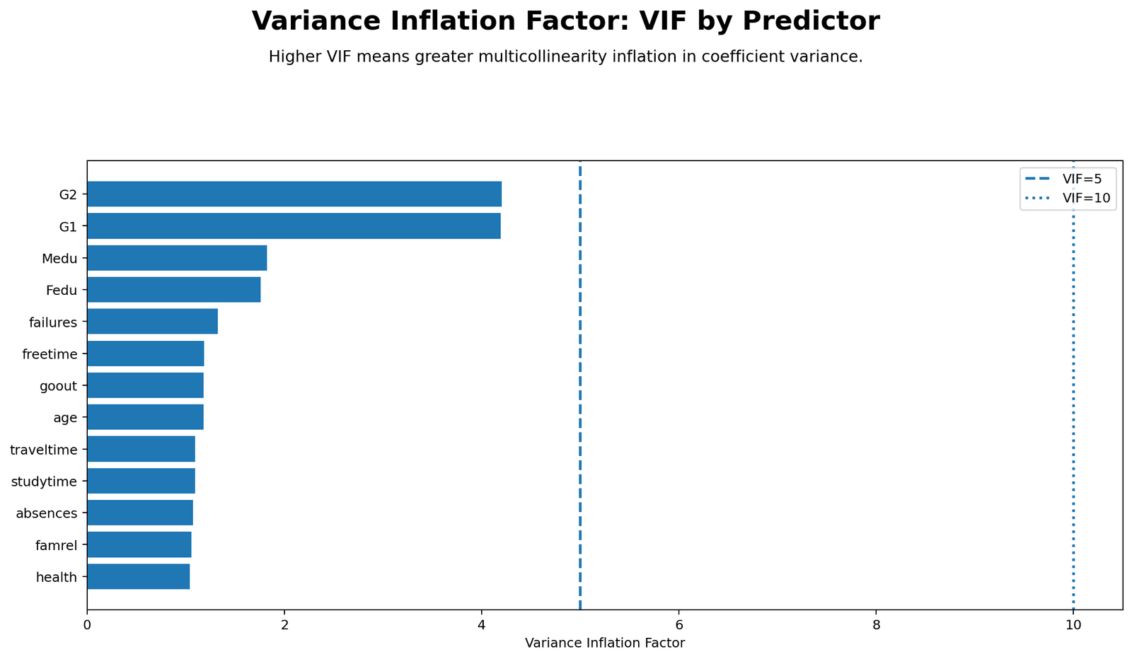
This chart ranks predictors by Variance Inflation Factor. The highest values are G2 = 4.204 and G1 = 4.195. These two bars are visibly longer than all other predictors, which means previous grade variables share a large amount of information with each other and with the remaining predictors. However, both remain below the dashed VIF = 5 threshold. That means the model does not cross the common moderate multicollinearity warning line.
Medu and Fedu are the next largest predictors, with VIF values around 1.82 and 1.76. These values are not concerning, but they make sense because mother education and father education are related. All other predictors are close to VIF = 1, meaning they have relatively high unique variance. This chart supports the final decision that multicollinearity is acceptable, while still identifying G1 and G2 as the main variables to watch.
Python Chart 2: Tolerance Cross-check
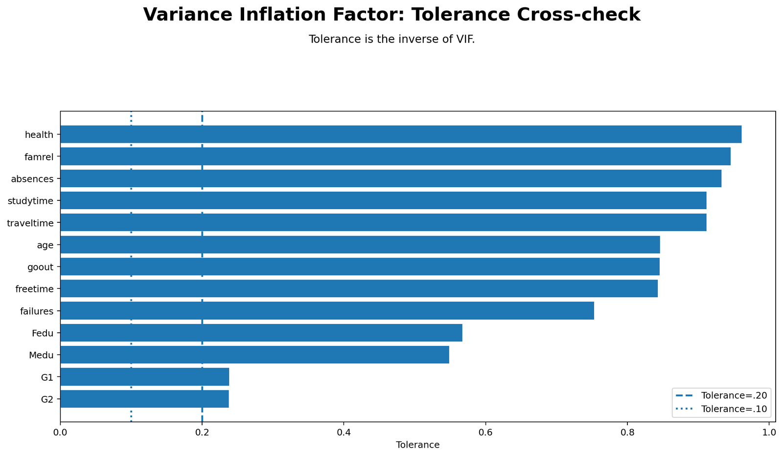
Tolerance is the inverse of VIF, so this chart verifies the same result from the opposite direction. The lowest tolerance values are for G1 and G2, both around .238. The dashed reference line at .20 marks the common warning threshold, while .10 marks a serious warning threshold. Since all predictors remain above .20, the tolerance cross-check agrees with the VIF chart.
The highest tolerance is for health = .961, followed by famrel and absences. These high tolerance values show that those predictors are not strongly explained by the other predictors. The tolerance chart is useful because it avoids a common reporting mistake: saying VIF is acceptable while ignoring tolerance. In this model, both diagnostics tell the same story: no predictor violates the selected multicollinearity rule.
Python Chart 3: Predictor Correlation Matrix
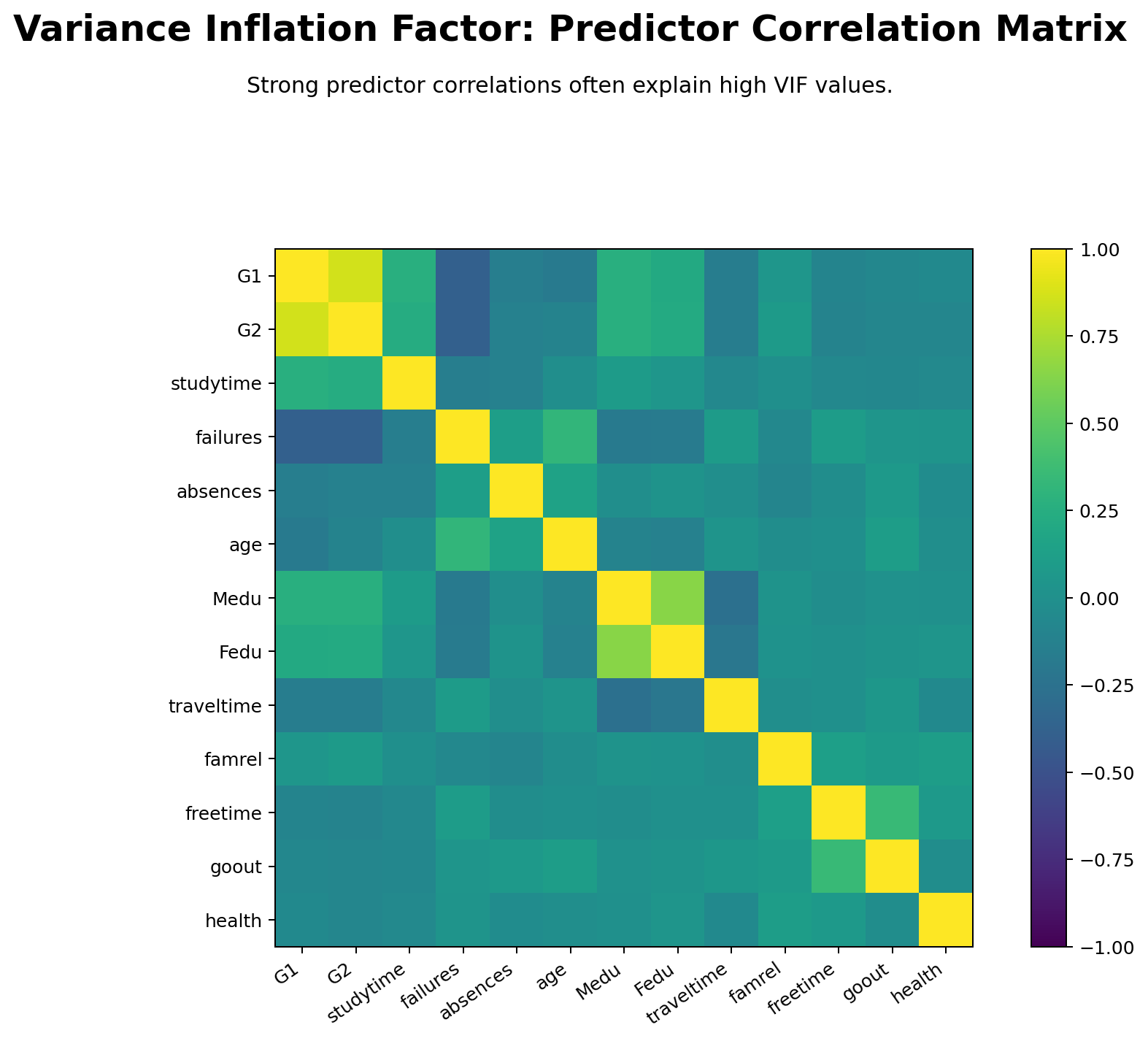
The predictor correlation heatmap explains why some predictors have higher VIF values than others. The brightest off-diagonal relationship is G1 and G2, with a correlation of about .865. This is the main reason both grade predictors have VIF values around 4.20. The next strong relationship is Medu and Fedu, with a correlation of about .647, which explains their mild VIF elevation.
The heatmap also shows moderate relationships such as freetime and goout, G1/G2 with failures, and failures with age. These correlations do not create dangerous VIF values in this model, but they provide context. A VIF table alone tells which predictor is inflated; the correlation matrix helps explain why it is inflated.
Python Chart 4: Strongest Predictor Correlations
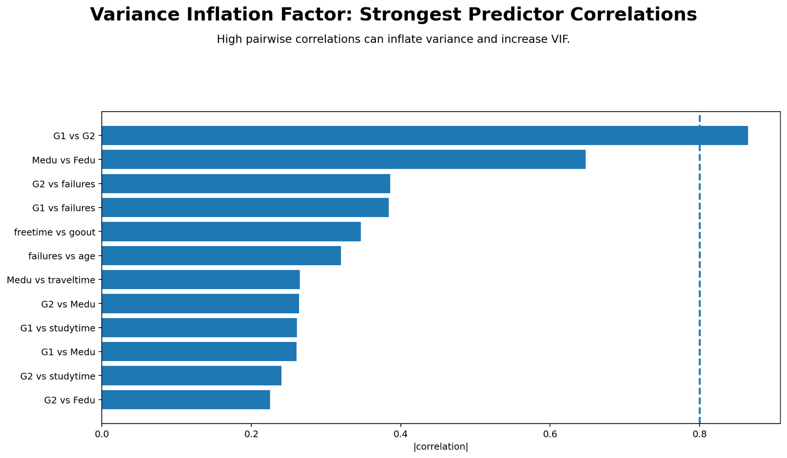
This chart isolates the strongest pairwise predictor correlations. The strongest relationship is G1 vs G2, which is above the .80 reference line. This confirms that the previous grade predictors are highly related. The second strongest relationship is Medu vs Fedu, around .65. Other relationships are below .40 and are less likely to create severe multicollinearity by themselves.
This chart is important because VIF is not only about pairwise correlations. A predictor can have high VIF because it is explained by a combination of multiple predictors, even if no single pairwise correlation is extreme. Still, the top-pair chart is useful here because the G1-G2 relationship is strong enough to explain the highest VIF values directly. The model remains acceptable, but this chart justifies the caution statement for G1 and G2.
Python Chart 5: VIF vs Tolerance
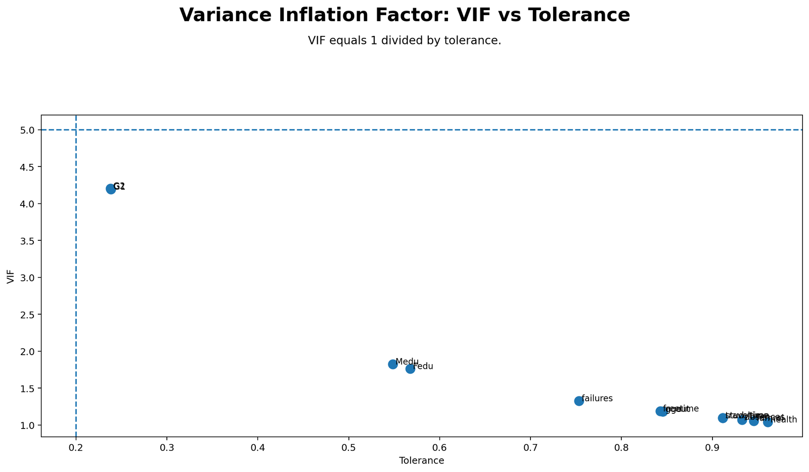
This scatter plot shows the mathematical connection between VIF and tolerance. Predictors with low tolerance have high VIF. G1 and G2 sit in the upper-left region because their tolerance is lowest and their VIF is highest. However, they are still below the horizontal VIF = 5 warning line and above the tolerance warning line.
Most other predictors cluster near VIF = 1 and tolerance close to 1. This cluster means those predictors are not strongly redundant with the rest of the model. The chart is useful in teaching because it shows that VIF and tolerance are not separate problems; they are inverse measures of the same multicollinearity concept.
Python Chart 6: Regression Coefficients
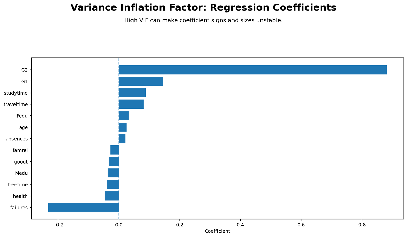
This chart shows the regression coefficients. G2 has the largest positive coefficient, which matches the SPSS output where B = .881 and Beta = .795. G1 is also positive, with B = .146. Failures has a negative coefficient, B = -.232, meaning more prior failures are associated with lower predicted G3 after controlling for the other predictors.
The chart connects coefficient interpretation with VIF. When VIF is high, coefficient size and sign can become unstable. In this model, VIF is acceptable, but G1 and G2 are still correlated enough that their coefficients should be described as adjusted effects in the presence of the other grade variable. The coefficient chart does not replace the VIF table; it helps explain why multicollinearity matters for interpretation.
Python Chart 7: VIF Decision Summary
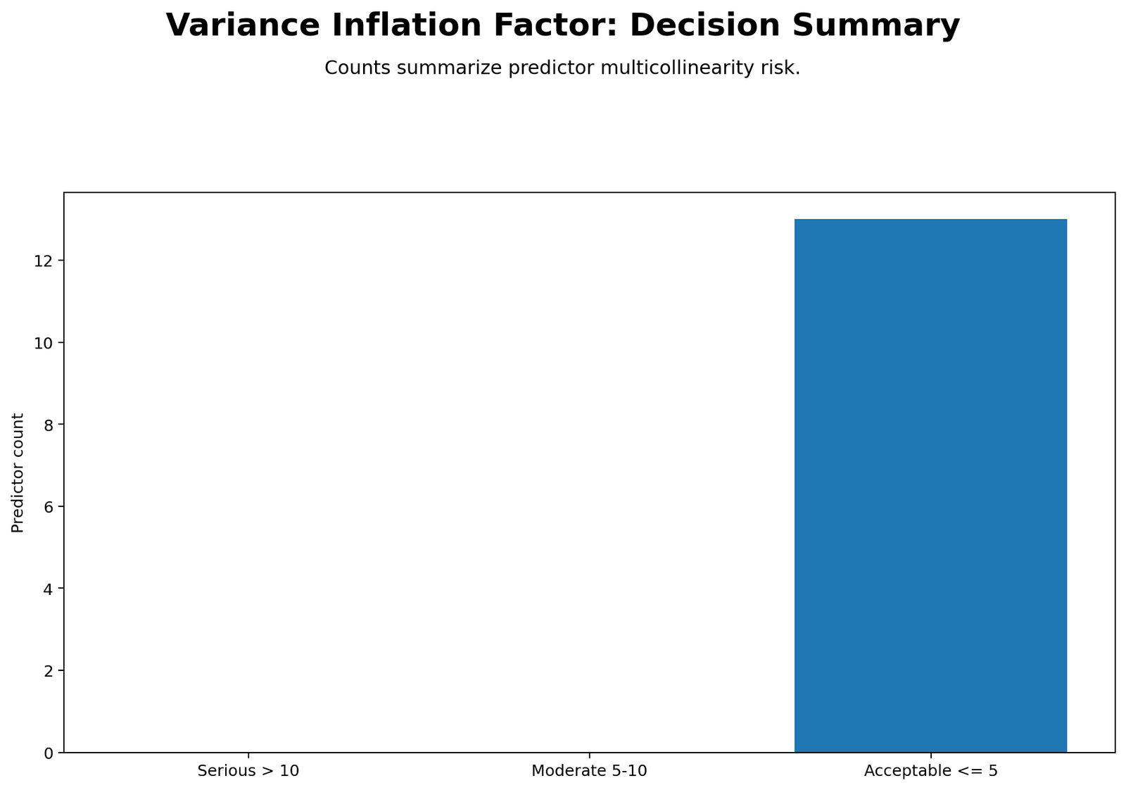
The decision summary chart gives the final diagnostic result: all 13 predictors fall in the acceptable VIF ≤ 5 category. No predictor falls in the moderate 5–10 category, and no predictor falls in the serious > 10 category. This chart is the easiest visual for a final report because it summarizes the VIF decision clearly.
The conclusion is not that multicollinearity is absent. The conclusion is that multicollinearity is not severe under the selected threshold. G1 and G2 still deserve caution because they are close to 5, but the model does not require immediate removal of predictors based on VIF alone.
R Chart-by-Chart Validation
The R charts validate the same VIF analysis using a separate software workflow. The R charts match the Python interpretation: G1 and G2 are the highest VIF predictors, tolerance remains above .20 for all predictors, and the final decision is acceptable multicollinearity.
R Chart 1: VIF by Predictor
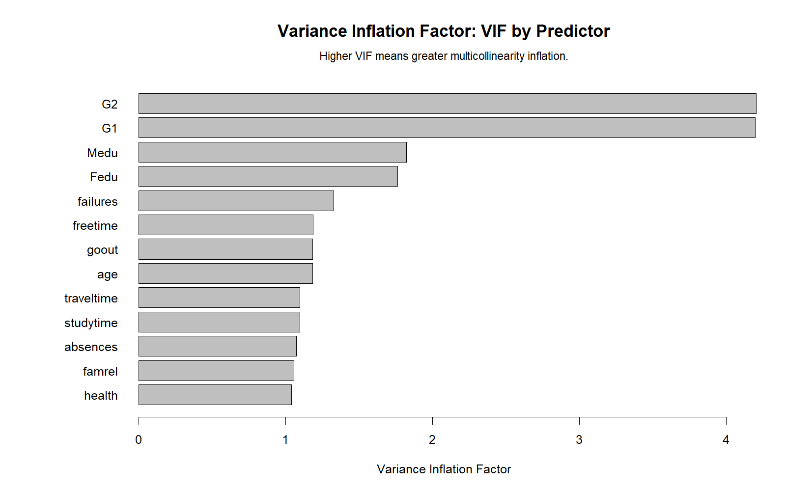
The R VIF chart reproduces the same ranking as Python and SPSS. G2 and G1 have the largest VIF values, both around 4.2, while all remaining predictors are below 2. This validates the conclusion that multicollinearity is concentrated mainly in the previous grade predictors, not across the entire predictor set.
R Chart 2: Tolerance Cross-check
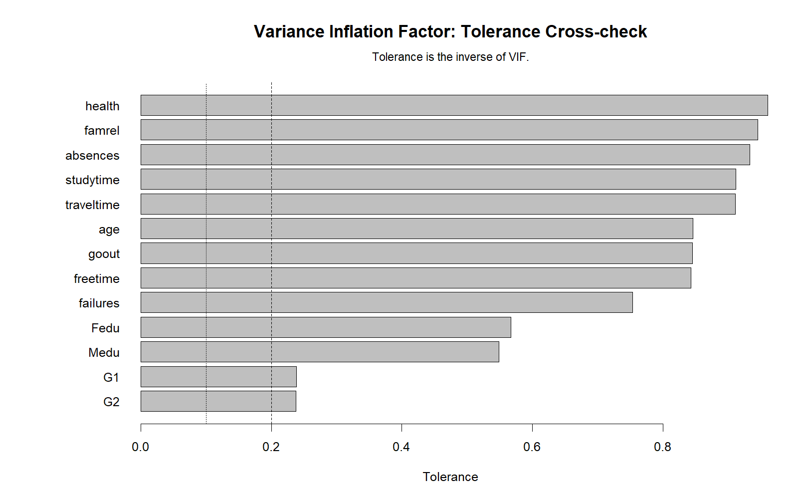
The R tolerance chart confirms that all predictors remain above the .20 warning threshold. G1 and G2 have the lowest tolerance, but their values remain acceptable. Health, famrel and absences have high tolerance values, showing low overlap with the rest of the predictors.
R Chart 3: Predictor Correlation Matrix
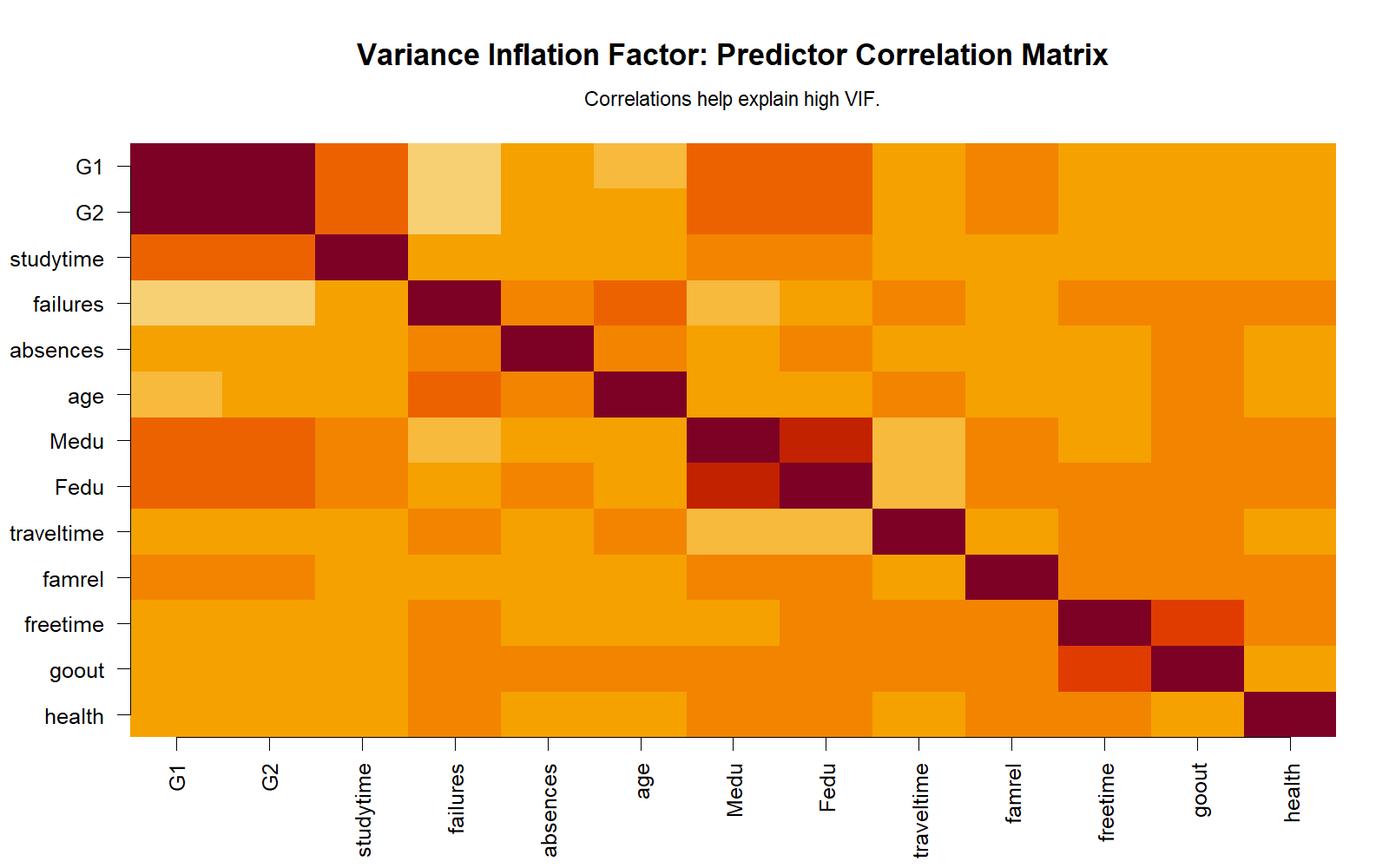
The R heatmap validates the same predictor relationship structure. The strongest off-diagonal correlation is between G1 and G2. Medu and Fedu are also related, and freetime and goout show a moderate relationship. The heatmap supports the VIF story because predictor correlations explain why some variables have higher inflation than others.
R Chart 4: Strongest Predictor Correlations
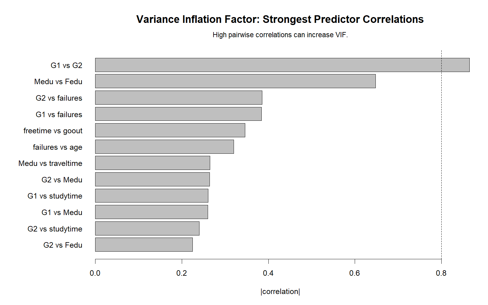
The R top-correlation chart again identifies G1 vs G2 as the strongest predictor pair. The value is above .80, which is high enough to explain why the two variables have the largest VIF values. Medu vs Fedu is the next strongest pair, explaining their mild VIF elevation. The remaining pairs are below levels that usually produce major VIF concern.
R Chart 5: VIF vs Tolerance
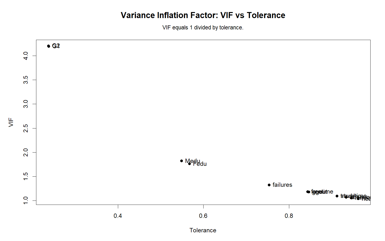
The R scatter plot confirms the inverse VIF-tolerance relationship. G1 and G2 appear as the highest VIF and lowest tolerance predictors. The remaining predictors cluster near VIF = 1 and high tolerance. This validates the Python scatter plot and confirms that the VIF calculation is consistent across software.
R Chart 6: Regression Coefficients
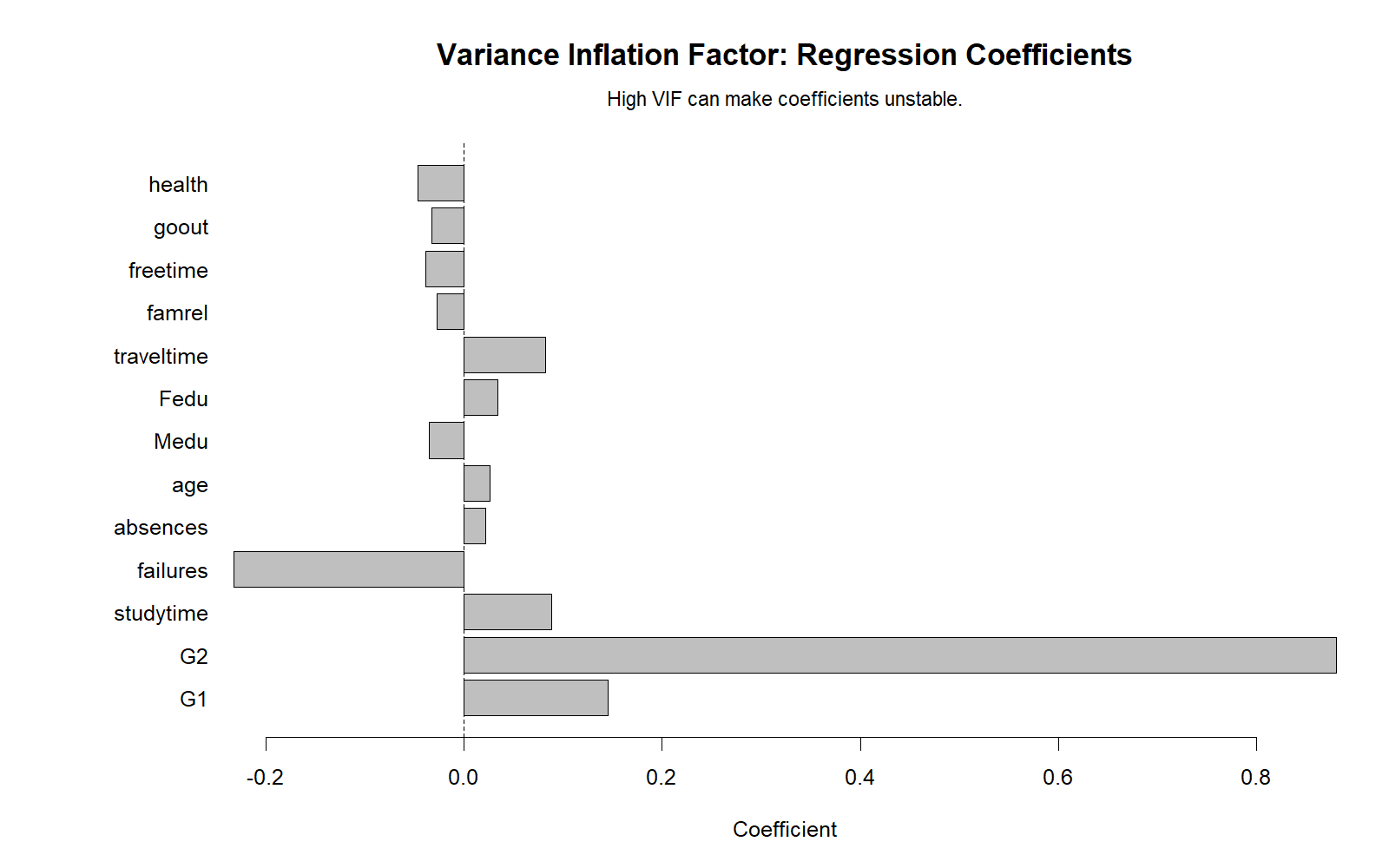
The R coefficient chart confirms the same coefficient direction as SPSS and Python. G2 has the strongest positive coefficient, G1 has a smaller positive coefficient, and failures has a negative coefficient. Since VIF is acceptable, these coefficients can be reported, but the interpretation of G1 and G2 should remain cautious because they measure related academic performance stages.
R Chart 7: VIF Decision Summary
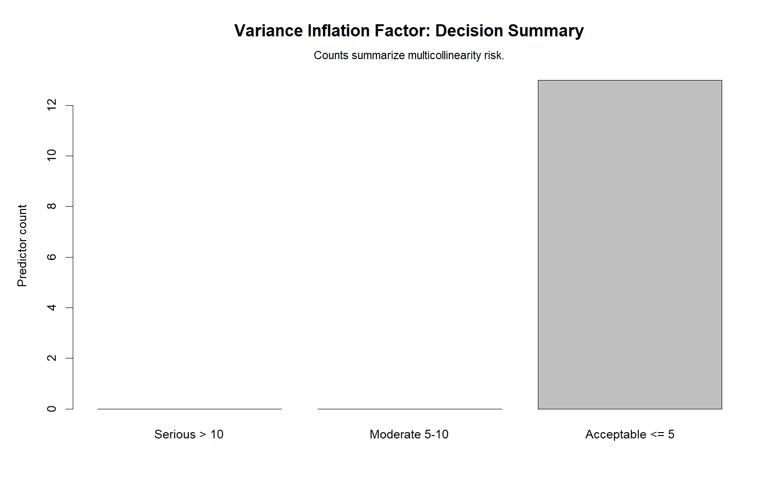
The R decision summary confirms that all predictors fall in the acceptable category. No predictor crosses the VIF = 5 or VIF = 10 threshold. This independent validation strengthens the final conclusion: the regression model has acceptable multicollinearity under the selected diagnostic rule.
SPSS, R, Python and Excel Workflows for Variance Inflation Factor
The same VIF logic can be applied in SPSS, R, Python and Excel. SPSS reports VIF directly in the regression Coefficients table. R and Python calculate VIF from auxiliary regressions. Excel can reproduce the same idea manually by regressing each predictor on all other predictors and using the VIF formula.
SPSS Workflow
| Step | SPSS Menu or Syntax | Purpose |
|---|---|---|
| Open dataset | File > Open > Data | Load the clean SPSS-ready dataset. |
| Run regression | Analyze > Regression > Linear | Set G3 as dependent variable and enter predictors. |
| Select collinearity diagnostics | Statistics > Collinearity diagnostics | Request tolerance, VIF and condition index output. |
| Read coefficients table | Coefficients > Collinearity Statistics | Use Tolerance and VIF columns for the decision. |
| Read condition index | Collinearity Diagnostics table | Check whether high condition index values involve multiple predictors. |
| Export output | File > Export or OUTPUT EXPORT | Save SPSS output PDF for reporting and verification. |
R Workflow
| Step | R Action | Purpose |
|---|---|---|
| Read data | read.csv() | Load the dataset. |
| Fit model | lm(G3 ~ predictors) | Fit the regression model. |
| Calculate VIF | car::vif(model) | Calculate VIF values for all predictors. |
| Calculate tolerance | 1 / vif_values | Cross-check VIF using tolerance. |
| Inspect correlations | cor() | Explain why VIF values are higher for some predictors. |
| Build charts | Base R or ggplot2 | Create VIF, tolerance, correlation, coefficient and decision charts. |
Python Workflow
| Step | Python Action | Purpose |
|---|---|---|
| Read data | pandas.read_csv() | Load the dataset into a DataFrame. |
| Select predictors | Create predictor list | Use the same predictors as SPSS and R. |
| Add constant if needed | statsmodels.add_constant() | Prepare model matrix for regression and VIF. |
| Calculate VIF | variance_inflation_factor() | Compute VIF for each predictor. |
| Calculate tolerance | 1 / VIF | Cross-check VIF results. |
| Create plots | matplotlib | Generate WordPress chart figures. |
Excel Workflow
| Excel Task | Formula or Tool | Purpose |
|---|---|---|
| Enable regression tool | Data Analysis ToolPak | Use Excel regression for auxiliary models. |
| Choose one predictor as outcome | Example: G2 as Y | Predict G2 from all other predictors. |
| Run auxiliary regression | Regression tool | Get R Square for that predictor. |
| Calculate tolerance | =1-RSQ | Find unique predictor variance after other predictors. |
| Calculate VIF | =1/(1-RSQ) | Calculate Variance Inflation Factor. |
| Repeat for every predictor | Auxiliary regressions | Create full VIF table. |
Code Blocks for Variance Inflation Factor
SPSS Syntax for VIF
* Variance Inflation Factor and Tolerance in SPSS.
* Dependent variable: G3.
* Predictors: G1 G2 studytime failures absences age Medu Fedu traveltime famrel freetime goout health.

TITLE "Variance Inflation Factor and Tolerance through SPSS collinearity diagnostics".

REGRESSION
  /DEPENDENT G3
  /METHOD=ENTER G1 G2 studytime failures absences age Medu Fedu traveltime famrel freetime goout health
  /STATISTICS COEFF OUTS R ANOVA COLLIN TOL
  /CRITERIA=PIN(.05) POUT(.10)
  /NOORIGIN.

CORRELATIONS
  /VARIABLES=G1 G2 studytime failures absences age Medu Fedu traveltime famrel freetime goout health
  /PRINT=TWOTAIL NOSIG
  /MISSING=PAIRWISE.

DESCRIPTIVES VARIABLES=G1 G2 studytime failures absences age Medu Fedu traveltime famrel freetime goout health
  /STATISTICS=MEAN STDDEV MIN MAX.

OUTPUT EXPORT
  /CONTENTS EXPORT=VISIBLE
  /PDF DOCUMENTFILE="Variance-Inflation-Factor-SPSS-Output.pdf".
Python Code for VIF
import pandas as pd
import statsmodels.api as sm
from statsmodels.stats.outliers_influence import variance_inflation_factor

df = pd.read_csv("dataset.csv")

dependent = "G3"
predictors = [
    "G1", "G2", "studytime", "failures", "absences", "age",
    "Medu", "Fedu", "traveltime", "famrel", "freetime", "goout", "health"
]

# Keep numeric data only and remove missing rows
model_data = df[[dependent] + predictors].apply(pd.to_numeric, errors="coerce").dropna()

X = model_data[predictors]
X_const = sm.add_constant(X)

# Fit regression model
y = model_data[dependent]
model = sm.OLS(y, X_const).fit()
print(model.summary())

# Calculate VIF and tolerance
vif_rows = []
for i, variable in enumerate(X_const.columns):
    if variable == "const":
        continue
    vif_value = variance_inflation_factor(X_const.values, i)
    tolerance = 1 / vif_value
    vif_rows.append({
        "predictor": variable,
        "VIF": vif_value,
        "Tolerance": tolerance,
        "Decision": "Acceptable" if vif_value <= 5 else "Review"
    })

vif_table = pd.DataFrame(vif_rows).sort_values("VIF", ascending=False)
print(vif_table)

# Predictor correlation matrix
corr_matrix = X.corr()
print(corr_matrix)

# Top absolute pairwise correlations
pairs = []
for i, col1 in enumerate(predictors):
    for col2 in predictors[i+1:]:
        pairs.append({
            "pair": f"{col1} vs {col2}",
            "correlation": corr_matrix.loc[col1, col2],
            "abs_correlation": abs(corr_matrix.loc[col1, col2])
        })

top_pairs = pd.DataFrame(pairs).sort_values("abs_correlation", ascending=False)
print(top_pairs.head(12))
R Code for VIF
# Variance Inflation Factor in R

df <- read.csv("dataset.csv")

predictors <- c(
  "G1", "G2", "studytime", "failures", "absences", "age",
  "Medu", "Fedu", "traveltime", "famrel", "freetime", "goout", "health"
)

vars_needed <- c("G3", predictors)
df_model <- df[vars_needed]
df_model[] <- lapply(df_model, as.numeric)
df_model <- na.omit(df_model)

model <- lm(
  G3 ~ G1 + G2 + studytime + failures + absences + age +
    Medu + Fedu + traveltime + famrel + freetime + goout + health,
  data = df_model
)

summary(model)

# Option 1: using car package
# install.packages("car")
library(car)
vif_values <- vif(model)

vif_table <- data.frame(
  predictor = names(vif_values),
  VIF = as.numeric(vif_values),
  Tolerance = 1 / as.numeric(vif_values)
)

vif_table <- vif_table[order(-vif_table$VIF), ]
print(vif_table)

# Predictor correlations
corr_matrix <- cor(df_model[predictors], use = "complete.obs")
print(corr_matrix)

# Top absolute pairwise correlations
pair_rows <- list()
k <- 1

for (i in 1:(length(predictors)-1)) {
  for (j in (i+1):length(predictors)) {
    pair_rows[[k]] <- data.frame(
      pair = paste(predictors[i], "vs", predictors[j]),
      correlation = corr_matrix[predictors[i], predictors[j]],
      abs_correlation = abs(corr_matrix[predictors[i], predictors[j]])
    )
    k <- k + 1
  }
}

top_pairs <- do.call(rbind, pair_rows)
top_pairs <- top_pairs[order(-top_pairs$abs_correlation), ]
head(top_pairs, 12)
Excel Formulas for VIF
Step 1:
Choose one predictor as the dependent variable in an auxiliary regression.

Example:
Predict G2 from G1, studytime, failures, absences, age, Medu, Fedu, traveltime, famrel, freetime, goout, health.

Step 2:
Get the R Square value from that auxiliary regression.

Step 3:
Calculate tolerance:
=1-R_Square

Step 4:
Calculate VIF:
=1/(1-R_Square)

Step 5:
Interpret:
If VIF <= 5, commonly acceptable.
If VIF is 5 to 10, moderate warning.
If VIF > 10, serious warning.

Example:
If auxiliary R Square = 0.762

Tolerance:
=1-0.762
=0.238

VIF:
=1/(1-0.762)
=4.202
APA Reporting Wording for Variance Inflation Factor
When reporting VIF, include the threshold rule, the highest VIF value, the lowest tolerance value, and the final decision. If the model includes closely related predictors such as G1 and G2, mention that their coefficients should be interpreted cautiously even when the VIF threshold is acceptable.
APA-Style VIF Report
Multicollinearity was assessed using tolerance and Variance Inflation Factor values. The regression model predicted G3 from G1, G2, studytime, failures, absences, age, Medu, Fedu, traveltime, famrel, freetime, goout and health. The highest VIF was observed for G2 (VIF = 4.204), followed by G1 (VIF = 4.195). The lowest tolerance value was .238. Since all VIF values were below 5 and all tolerance values were above .20, the model did not show harmful multicollinearity under the selected diagnostic rule. However, G1 and G2 were strongly correlated and should be interpreted with caution.
Full Model Report Sentence
The overall regression model was statistically significant, F(13, 635) = 281.518, p < .001, and explained 85.2% of the variance in G3, R² = .852, adjusted R² = .849. Collinearity diagnostics indicated acceptable multicollinearity, with all VIF values below 5 and all tolerance values above .20. The highest VIF values were for G2 (VIF = 4.204) and G1 (VIF = 4.195), indicating elevated but acceptable overlap between previous grade predictors.
Short Reporting Sentences
- VIF decision: All predictors had VIF values below 5, so harmful multicollinearity was not detected.
- Tolerance decision: All tolerance values were above .20, supporting the same conclusion.
- Main caution: G1 and G2 had the highest VIF values because they were strongly correlated.
- Practical conclusion: The model can be reported, but coefficients for G1 and G2 should be interpreted as adjusted effects in the presence of each other.
Common Mistakes in VIF Interpretation
Variance Inflation Factor is easy to calculate, but interpretation mistakes are common. The biggest mistake is treating VIF as a model-fit statistic. VIF does not say whether the model is good or bad overall. It says whether predictors overlap too much for stable coefficient interpretation.
| Mistake | Why It Is a Problem | Correct Practice |
|---|---|---|
| Thinking high R² means no multicollinearity | A model can have high R² and still have unstable coefficients. | Check VIF and tolerance separately from model fit. |
| Using only pairwise correlations | VIF can be high because of combined predictor overlap, not only one pair. | Use both VIF and correlation matrix. |
| Deleting predictors automatically when VIF is high | A predictor may be theoretically important. | Review purpose, theory, prediction goal, and coefficient stability. |
| Ignoring tolerance | Tolerance is the inverse diagnostic and can reveal the same issue clearly. | Report both VIF and tolerance when possible. |
| Using VIF for the dependent variable | VIF applies to predictors, not the outcome variable. | Calculate VIF only for independent variables in a regression model. |
| Assuming VIF checks normality | VIF checks multicollinearity, not residual distribution. | Use normality and residual diagnostics separately. |
| Ignoring condition index | SPSS may show additional collinearity structure beyond simple VIF. | Review condition index and variance proportions when available. |
Key reminder: VIF is part of regression assumption checking. It should be interpreted with residual plots, linearity checks, homoscedasticity tests, normality diagnostics, and model specification checks such as the Ramsey RESET test and Goldfeld-Quandt test.
When to Use Variance Inflation Factor
Use Variance Inflation Factor whenever a regression model has multiple predictors and you need to know whether predictor overlap is inflating coefficient variance. VIF is especially important when the goal is interpretation rather than only prediction.
| Use VIF When | Why It Matters | Example from This Guide |
|---|---|---|
| You run multiple regression | Multiple predictors can overlap and make coefficients unstable. | G3 was predicted from 13 predictors. |
| You include similar predictors | Similar predictors often share variance. | G1 and G2 are both previous grade variables. |
| You want coefficient interpretation | High VIF can inflate standard errors and weaken interpretability. | G1 and G2 require careful adjusted interpretation. |
| You see unexpected coefficient signs | Multicollinearity can produce unstable signs or sizes. | Some small coefficients should be interpreted with the full predictor set in mind. |
| You prepare a regression assumptions section | VIF is a standard assumption check for multicollinearity. | All predictors passed the VIF ≤ 5 rule. |
| You compare SPSS, R, Python and Excel output | VIF should match across software when the same model is used. | SPSS, Python and R results all support the same decision. |
Do not use VIF as a substitute for variance, spread, or reliability measures. If you need to compare relative variability across variables, use the coefficient of variation. If you need confidence intervals for coefficients or means, use the confidence interval guide. If you need practical importance, use effect size.
Downloads and Resources for Variance Inflation Factor
The SPSS output PDF below verifies the regression model, VIF values, tolerance values, collinearity diagnostics, predictor correlation matrix and descriptive statistics used in this guide.
Download SPSS Output PDF
Verified SPSS output for Variance Inflation Factor, tolerance, regression coefficients, collinearity diagnostics and predictor correlations.
Copy VIF Code
Use the SPSS, Python, R and Excel code blocks to reproduce the Variance Inflation Factor analysis.
Download note: Use the SPSS PDF as the official verification file. The Python and R charts provide visual interpretation and software validation for the same VIF decision.
FAQs About Variance Inflation Factor
What is Variance Inflation Factor?
Variance Inflation Factor is a regression diagnostic that measures how much a predictor’s coefficient variance is inflated because that predictor is correlated with other predictors in the model.
What is the VIF formula?
The VIF formula is VIF = 1 / (1 − R²j), where R²j comes from predicting one predictor using all the other predictors.
What is tolerance in VIF analysis?
Tolerance is the inverse of VIF. It is calculated as tolerance = 1 / VIF or 1 − R²j. Low tolerance means high multicollinearity risk.
What VIF value is acceptable?
A common rule is that VIF values below 5 are acceptable. Values from 5 to 10 are often treated as a moderate warning, and values above 10 are often treated as serious multicollinearity.
What tolerance value is acceptable?
A common rule is that tolerance should be above .20. Tolerance below .20 is a warning, and tolerance below .10 is often treated as serious multicollinearity.
What was the highest VIF in this example?
The highest VIF was for G2, with VIF = 4.204. G1 was very close, with VIF = 4.195.
Was multicollinearity a serious problem in this model?
No. All predictors had VIF values below 5 and tolerance values above .20. Therefore, the model did not show harmful multicollinearity under the selected VIF rule.
Why were G1 and G2 the highest VIF predictors?
G1 and G2 were the highest VIF predictors because they were strongly correlated. The predictor correlation matrix showed G1 vs G2 = .865.
Can a model have high R² and still have multicollinearity?
Yes. High R² describes model fit, while VIF describes predictor overlap. A model can predict well and still have unstable individual coefficients if predictors are highly correlated.
Does VIF test normality?
No. VIF checks multicollinearity among predictors. It does not test normality, residual distribution, skewness, kurtosis, or homoscedasticity.
Should I remove a predictor if VIF is high?
Not automatically. First check theory, research purpose, prediction goals, pairwise correlations, coefficient stability and whether the predictor is essential. Then decide whether to remove, combine, transform, or keep the variable.
How do I calculate VIF in SPSS?
In SPSS, run Linear Regression, click Statistics, and select Collinearity diagnostics. SPSS will show tolerance and VIF in the Coefficients table.
How do I calculate VIF in Python?
In Python, use statsmodels.stats.outliers_influence.variance_inflation_factor on the regression predictor matrix.
How do I calculate VIF in R?
In R, fit a regression model with lm() and then use car::vif(model) to calculate VIF values.
How do I calculate VIF in Excel?
In Excel, run an auxiliary regression for each predictor using all other predictors, record the R Square value, then calculate VIF = 1 / (1 − R²).

