Quick Answer: Durbin Watson Test Result

The verified SPSS output for the Durbin Watson Test uses a regression model predicting G3 final grade from G1, G2, studytime, failures and absences. The model is strong overall, with R = .922, R Square = .851, Adjusted R Square = .849, and standard error of the estimate = 1.254. The ANOVA table reports F(5, 643) = 731.966, p < .001, meaning the regression model explains a statistically significant amount of variation in G3.

The manual Durbin-Watson output reports N = 649, sum of squared residuals = 1010.68, sum of squared residual differences = 1877.18, and Durbin-Watson statistic = 1.85735. A Durbin-Watson value close to 2 usually indicates little or no first-order autocorrelation. The approximate lag-1 residual correlation is .07133, and the residual-lag correlation table reports r = .071, p = .072.

What Is the Durbin Watson Test?

Durbin Watson Test, often written as the Durbin-Watson test, is a regression diagnostic used to detect first-order autocorrelation in residuals. In regression, residuals should ideally be independent. If residuals are positively autocorrelated, one residual tends to be followed by a residual with the same sign. If residuals are negatively autocorrelated, one residual tends to be followed by a residual with the opposite sign.

The Durbin-Watson statistic usually ranges from 0 to 4. A value near 2 indicates little or no first-order autocorrelation. A value clearly below 2 suggests positive autocorrelation. A value clearly above 2 suggests negative autocorrelation. In this guide, the observed value is 1.85735, which is close to 2 and therefore does not indicate a serious residual autocorrelation problem.

Durbin-Watson belongs to the family of regression diagnostics. It should be interpreted with other regression checks such as residual histograms, residuals-versus-fitted plots, observed-versus-fitted plots, model specification checks such as the Ramsey RESET test, and heteroscedasticity checks such as the Goldfeld-Quandt test. If you are checking distribution assumptions before regression, also compare this guide with Q-Q plot normality check, P-P plot normality check, Kolmogorov-Smirnov test, Lilliefors test, D’Agostino-Pearson test, Cramer-von Mises test, and Ryan-Joiner test.

Durbin Watson Test Formula

The Durbin-Watson statistic compares the squared difference between consecutive residuals with the total squared residual variation. The formula is:

Here, eₜ is the residual at position t, and eₜ₋₁ is the residual immediately before it in the ordered dataset. If consecutive residuals are very similar, the numerator becomes smaller and the Durbin-Watson statistic moves below 2. If consecutive residuals frequently move in opposite directions, the numerator becomes larger and the statistic can move above 2.

For the verified SPSS output in this guide:

An approximate relationship between Durbin-Watson and lag-1 residual autocorrelation is:

Null and Alternative Hypotheses for the Durbin Watson Test

The Durbin Watson Test is usually framed around first-order residual autocorrelation. In a regression model, the residuals should be independent. The hypotheses can be written as follows:

Null Hypothesis

H₀: The regression residuals have no first-order autocorrelation.

Alternative Hypothesis

H₁: The regression residuals have first-order autocorrelation.

Some Durbin-Watson applications use a one-sided alternative, especially when the researcher is mainly concerned about positive autocorrelation. In this guide, the observed statistic of 1.85735 is slightly below 2, so the approximate residual autocorrelation is slightly positive. However, the approximate lag-1 correlation is small (.07133), and the residual-lag correlation is not significant at the .05 level (p = .072).

Dataset and Variables Used

The worked example uses a student performance regression model. The dependent variable is G3, which represents the final grade. The predictors are G1, G2, studytime, failures, and absences. The Durbin Watson Test is applied to the regression residuals from this model.

Before interpreting regression diagnostics, it is helpful to understand the dataset with descriptive statistics, frequency distribution, five-number summary, box plot interpretation, histogram interpretation, confidence interval, and effect size reporting.

Verified SPSS Output Interpretation

The verified SPSS output PDF for this guide is available here: Durbin Watson Test SPSS Output PDF. The output includes the regression model, model summary, ANOVA table, coefficient table, residual statistics, manual Durbin-Watson calculation, residual descriptives, normality diagnostics and lag-residual correlation.

SPSS Regression Model Summary

SPSS Coefficient Interpretation

SPSS Durbin-Watson Manual Statistic

SPSS Residual Diagnostics

Because regression diagnostics involve more than one assumption, the Durbin Watson result should be combined with residual distribution checks, residuals-versus-fitted plots, and additional assumption guides such as Ramsey RESET test, Goldfeld-Quandt test, Q-Q plot normality check, and histogram interpretation.

Python Chart-by-Chart Interpretation

The Python charts explain the Durbin Watson Test visually. They show observed versus fitted values, residual sequence behavior, lag-1 residual relationship, residual autocorrelation by lag, residual distribution, Durbin-Watson reference distribution and residuals versus fitted values.

Python Chart 1: Observed vs Fitted Values

Detailed interpretation

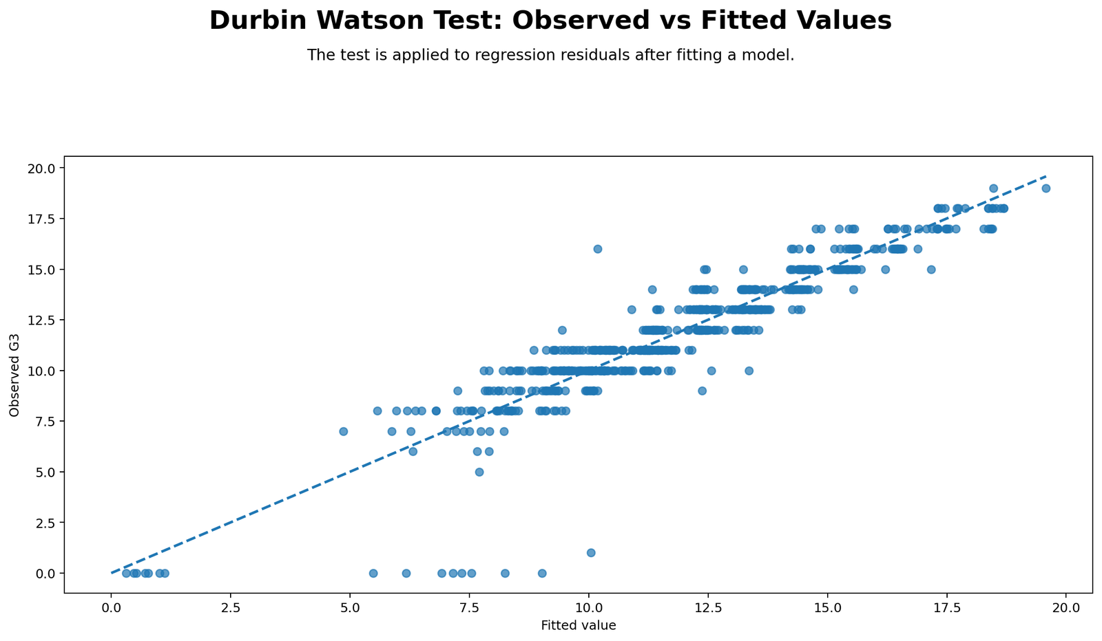
This chart checks the overall prediction quality of the regression model before focusing on autocorrelation. When points fall close to the diagonal pattern, fitted values are close to observed values. The SPSS model has R Square = .851, so the model explains a large share of G3 variation.

Observed-versus-fitted plots do not directly calculate the Durbin-Watson statistic, but they help show whether residuals are likely to be small or large. A strong fitted relationship makes the residual diagnostics more meaningful because the residuals represent what the model has not explained.

Decision/reporting conclusion: The observed-versus-fitted chart supports a strong regression model. Durbin-Watson diagnostics should therefore focus on whether the remaining residuals are independent across the sequence.

Python Chart 2: Residual Sequence Plot

Detailed interpretation

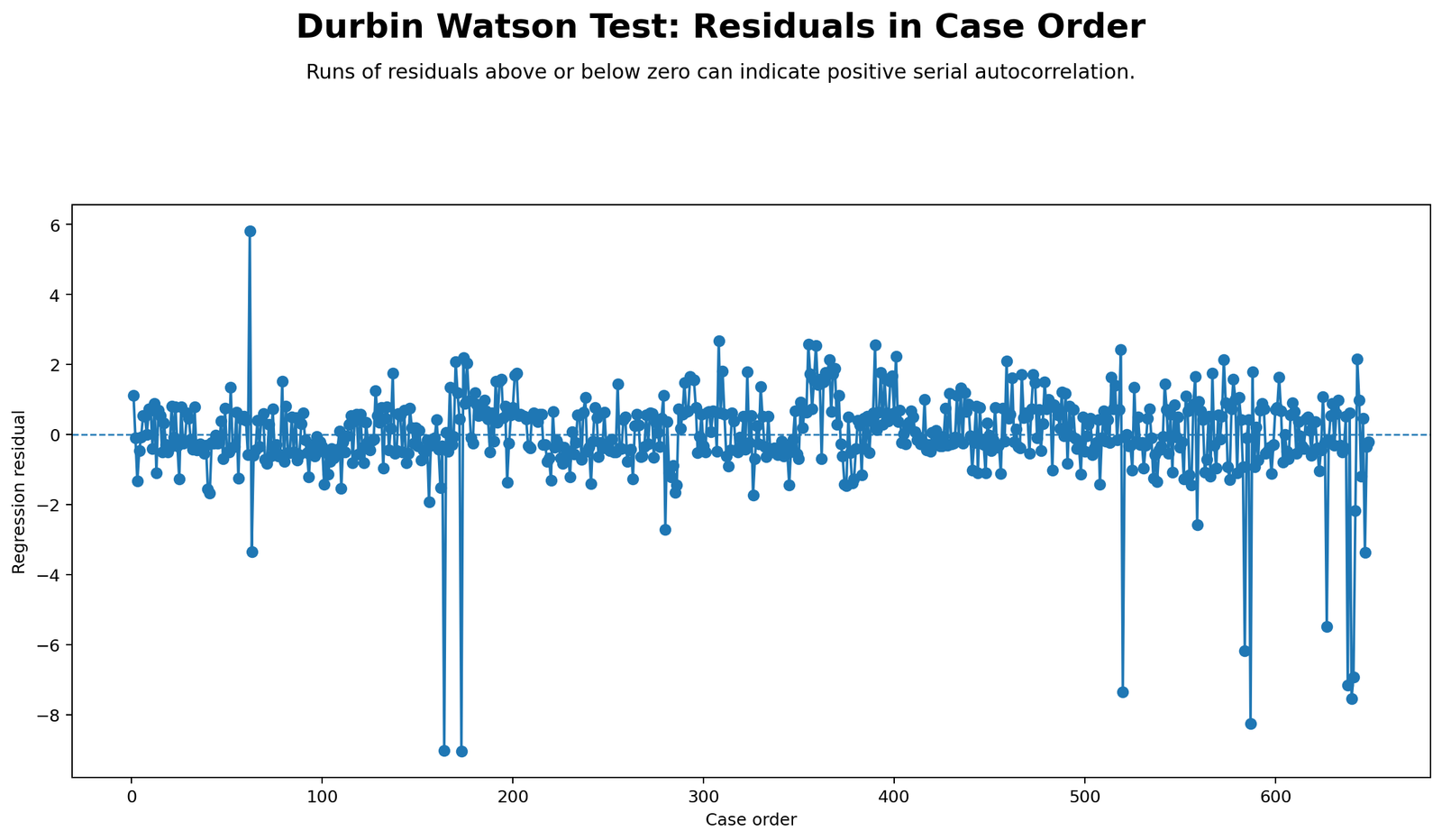
The residual sequence plot is central to Durbin-Watson interpretation because the test depends on consecutive residuals. If residuals appear in long runs above or below zero, that may indicate positive autocorrelation. If residuals alternate sharply between positive and negative values, that may indicate negative autocorrelation.

In this example, the residuals fluctuate around zero without an obvious long repeating wave pattern. Some residuals are large, especially on the negative side, which agrees with the SPSS residual minimum of -9.07158. However, large residuals are not the same as serial autocorrelation.

Decision/reporting conclusion: The residual sequence plot does not show strong repeated residual clustering. This supports the Durbin-Watson result of 1.85735, which is close to 2.

Python Chart 3: Lag-1 Residual Scatter

Detailed interpretation

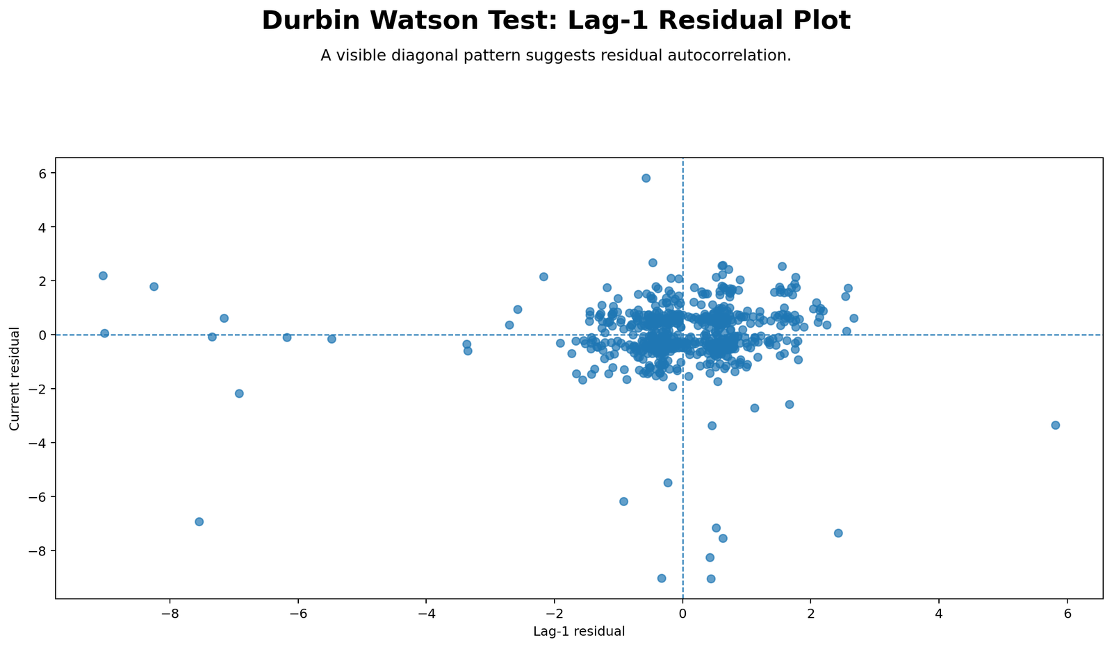
The lag-1 residual scatter plot directly visualizes first-order residual autocorrelation. If the points form a strong upward pattern, residuals are positively autocorrelated. If they form a strong downward pattern, residuals are negatively autocorrelated. A scattered cloud around zero indicates weak or no lag-1 autocorrelation.

The SPSS output reports an approximate lag-1 residual correlation of .07133, and the residual-lag correlation table reports r = .071, p = .072. This is a small positive relationship, not a strong autocorrelation pattern.

Decision/reporting conclusion: The lag-1 scatter supports a small, non-significant positive residual association. The residual independence assumption is not seriously violated.

Python Chart 4: Residual Autocorrelation by Lag

Detailed interpretation

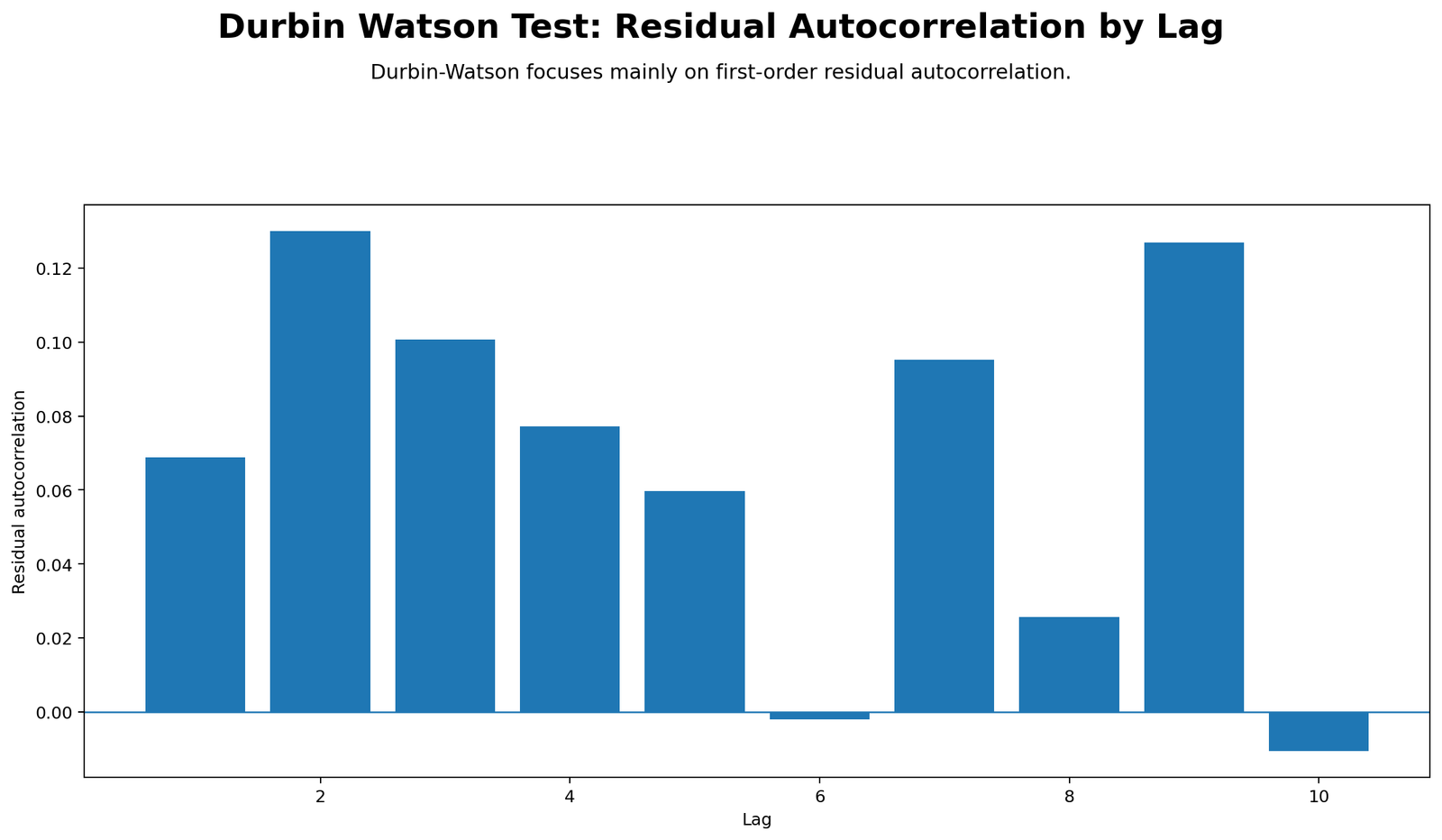
Although the Durbin Watson Test focuses mainly on first-order autocorrelation, the residual autocorrelation chart provides a wider diagnostic view. It shows whether residuals are related not only to the previous residual but also to residuals several positions earlier.

When autocorrelation bars stay close to zero and do not form a consistent pattern, the residual sequence does not show strong serial dependence. If several lags were large, a time-series or repeated-order model might be needed.

Decision/reporting conclusion: The autocorrelation-by-lag chart supports the conclusion that residual dependence is not severe. The Durbin-Watson value close to 2 is consistent with weak lag structure.

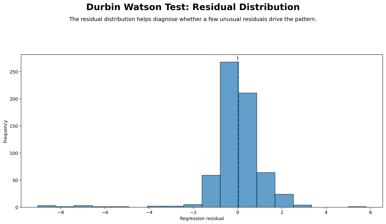
Python Chart 5: Residual Histogram

Detailed interpretation

This residual histogram checks the distribution shape of residuals. Durbin-Watson focuses on residual independence, not residual normality, but both are important regression diagnostics. The SPSS residual descriptives show residual mean near zero, standard deviation about 1.2489, skewness -2.844, and kurtosis 18.545.

The histogram helps explain why normality tests are significant even though autocorrelation is not severe. The residuals are centered near zero but have heavy tails and some extreme negative values.

Decision/reporting conclusion: The histogram indicates residual distribution issues, especially skewness and heavy tails. This does not overturn the Durbin-Watson independence conclusion, but it should be reported as a separate residual normality concern.

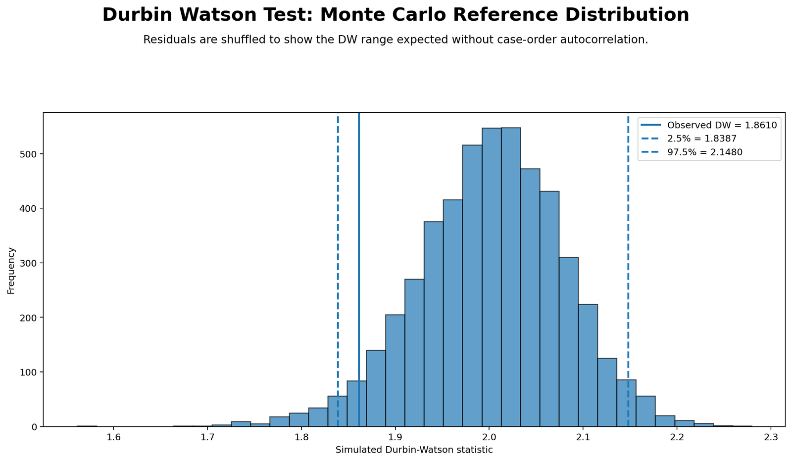
Python Chart 6: Durbin Watson Reference Distribution

Detailed interpretation

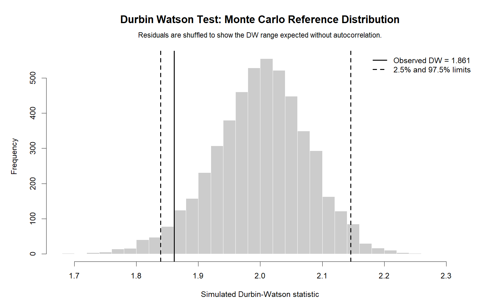
The reference distribution chart shows where the observed Durbin-Watson statistic sits relative to values expected under weak or no autocorrelation. The observed value of approximately 1.85735 is close to the central no-autocorrelation reference value of 2.

This visual display makes the interpretation easier for students and readers. A statistic near 2 is generally treated as acceptable, while values far below or far above 2 require additional investigation.

Decision/reporting conclusion: The observed Durbin-Watson statistic lies close to the no-autocorrelation region. The result supports retaining the residual independence assumption for practical regression reporting.

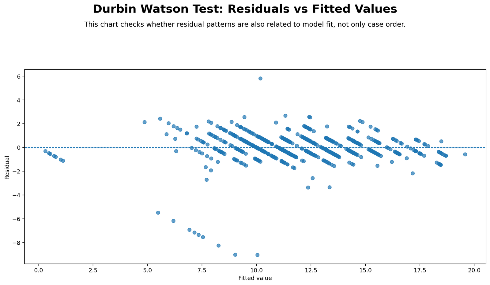
Python Chart 7: Residuals vs Fitted Values

Detailed interpretation

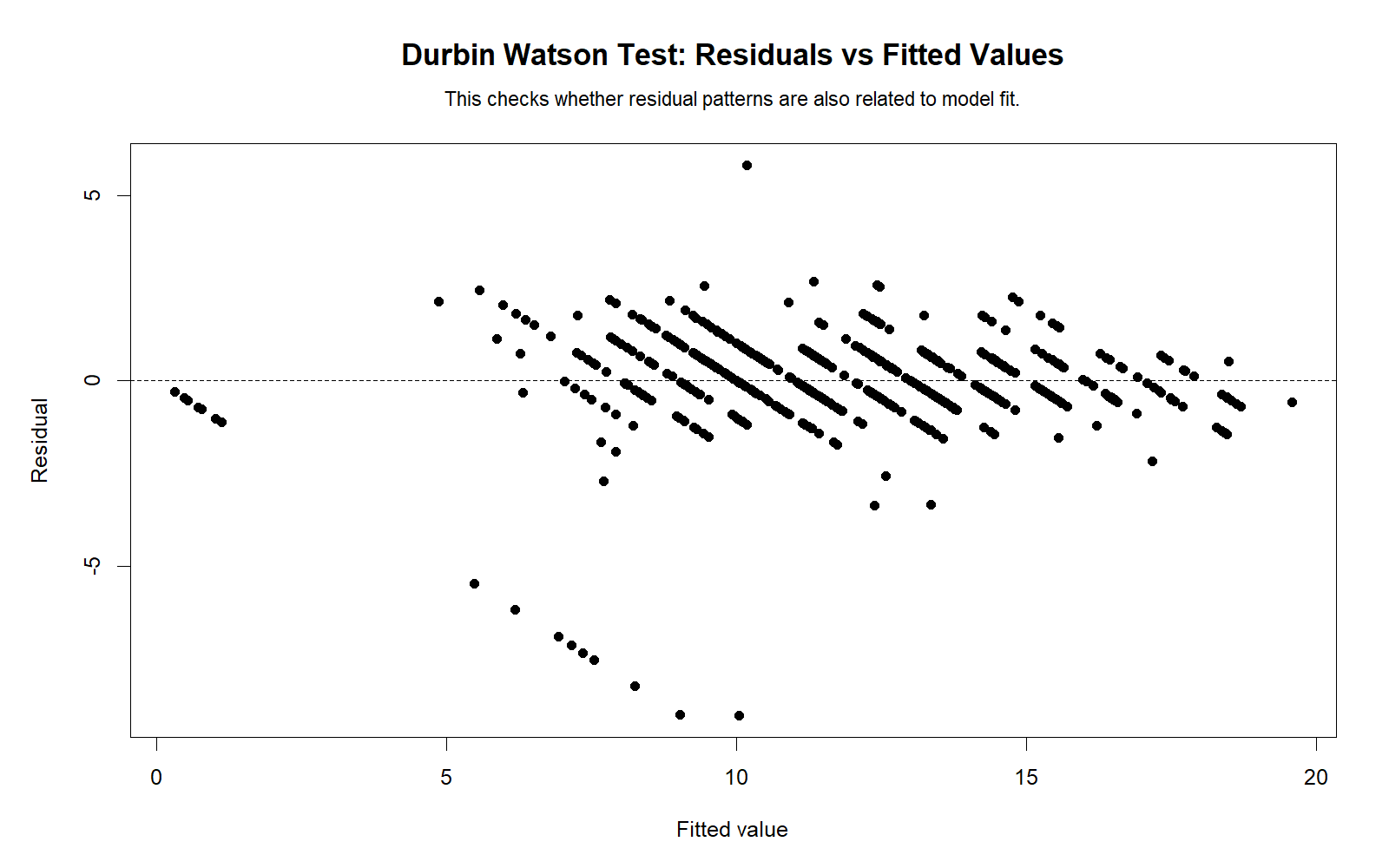
The residuals-versus-fitted plot checks whether residuals show nonlinearity, unequal spread or other systematic model patterns. Durbin-Watson focuses on residual order, but residuals-versus-fitted focuses on whether errors behave similarly across predicted values.

If residuals show a funnel shape, the model may have heteroscedasticity. If residuals show a curve, the model may be misspecified. This is why a complete regression report should not rely only on the Durbin Watson Test.

Decision/reporting conclusion: The residuals-versus-fitted plot should be used with the Durbin-Watson result. The main autocorrelation decision is acceptable, but residual distribution and model-pattern diagnostics should still be reviewed.

R Chart-by-Chart Validation

The R charts validate the same Durbin Watson Test interpretation using an independent workflow. This confirms that the Python charts and SPSS output tell the same story: the model fits G3 strongly, the Durbin-Watson statistic is close to 2, and there is no serious first-order residual autocorrelation.

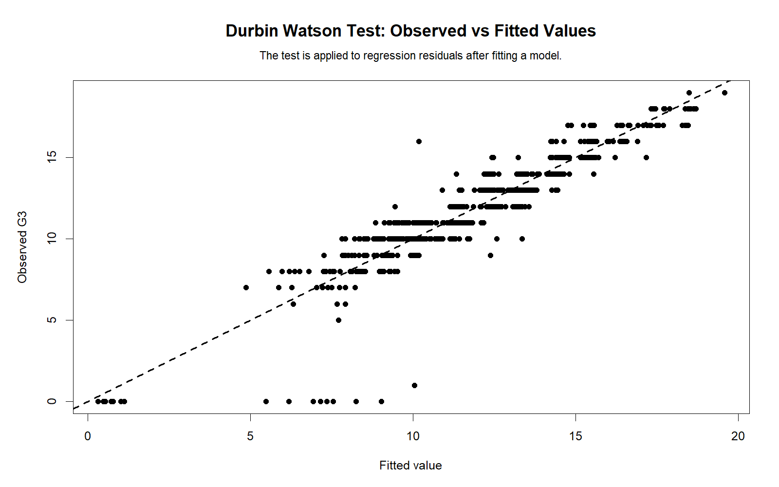
R Chart 1: Observed vs Fitted Values

Detailed interpretation

The R chart confirms that fitted G3 values align strongly with observed G3 values. This is consistent with the SPSS model summary, where R Square is .851. Strong model fit does not guarantee perfect residual behavior, but it provides the foundation for residual diagnostics.

Decision/reporting conclusion: R validates the strong model-fit context. Residual diagnostics should then focus on independence, normality, spread and model pattern.

R Chart 2: Residual Sequence Plot

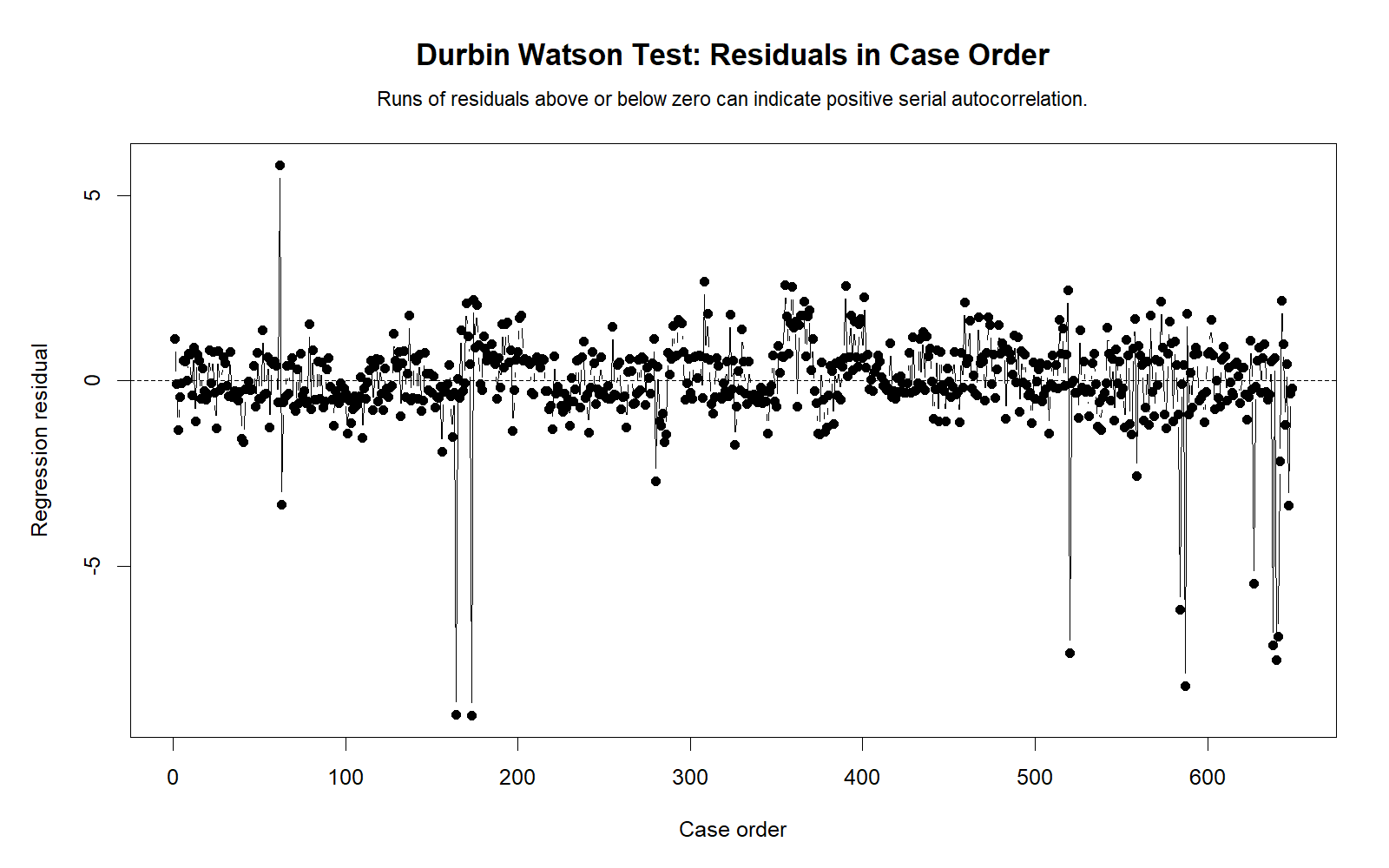
Detailed interpretation

The R residual sequence plot shows residuals fluctuating around zero. A severe autocorrelation problem would usually show long runs, waves or repeated clusters. The visual pattern is consistent with a Durbin-Watson statistic close to 2.

Decision/reporting conclusion: R confirms that the residual sequence does not show a strong serial pattern. The independence assumption is not seriously threatened by first-order autocorrelation.

R Chart 3: Lag-1 Residual Scatter

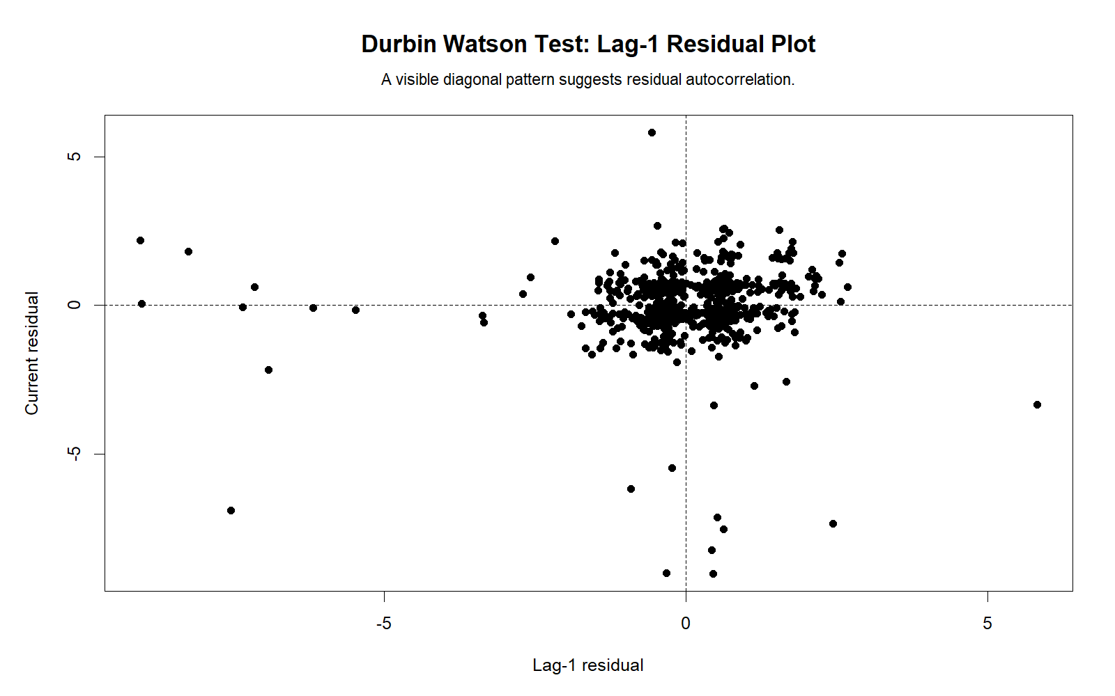
Detailed interpretation

This R chart confirms that the lag-1 residual relationship is weak. The SPSS diagnostic reports a small lag residual correlation of approximately .071, which is not significant at the .05 level.

Decision/reporting conclusion: R validates that current residuals are not strongly predicted by previous residuals. This supports the Durbin-Watson decision.

R Chart 4: Residual Autocorrelation by Lag

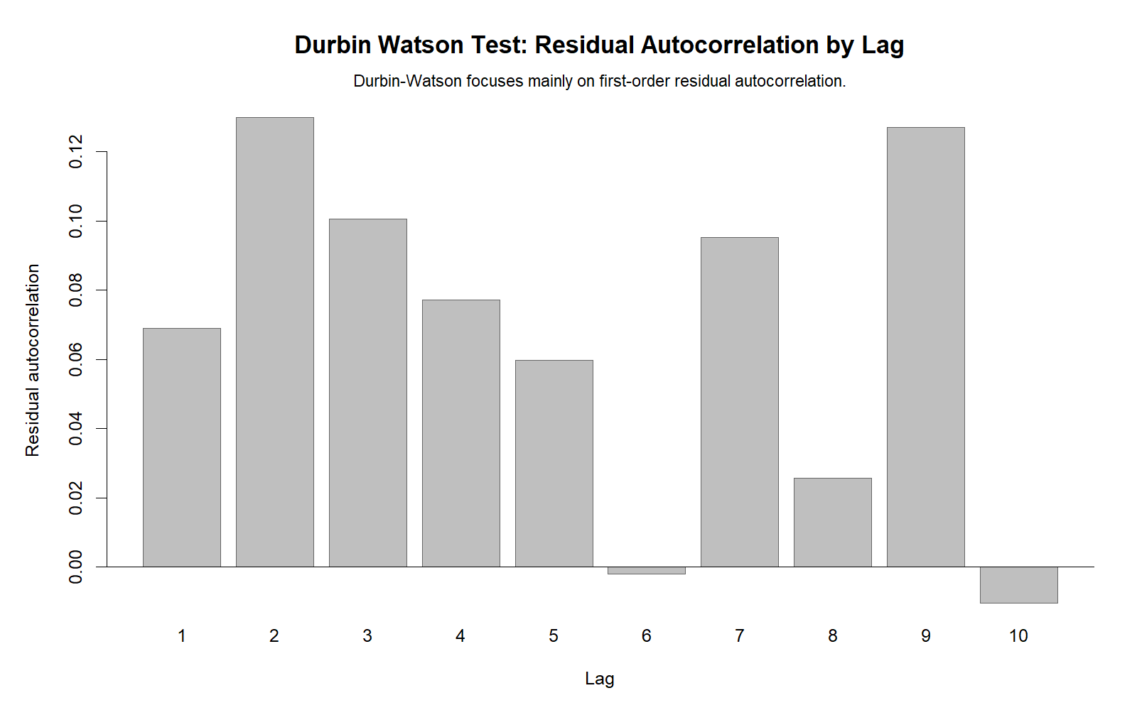
Detailed interpretation

The R autocorrelation-by-lag chart checks whether residual dependence appears beyond the first lag. Durbin-Watson focuses on lag 1, but multiple lag checks are useful when the observation order has time or sequence meaning.

Decision/reporting conclusion: R supports the conclusion that residual autocorrelation is not severe. If this were a true time-series dataset, additional autocorrelation tests could still be added.

R Chart 5: Residual Histogram

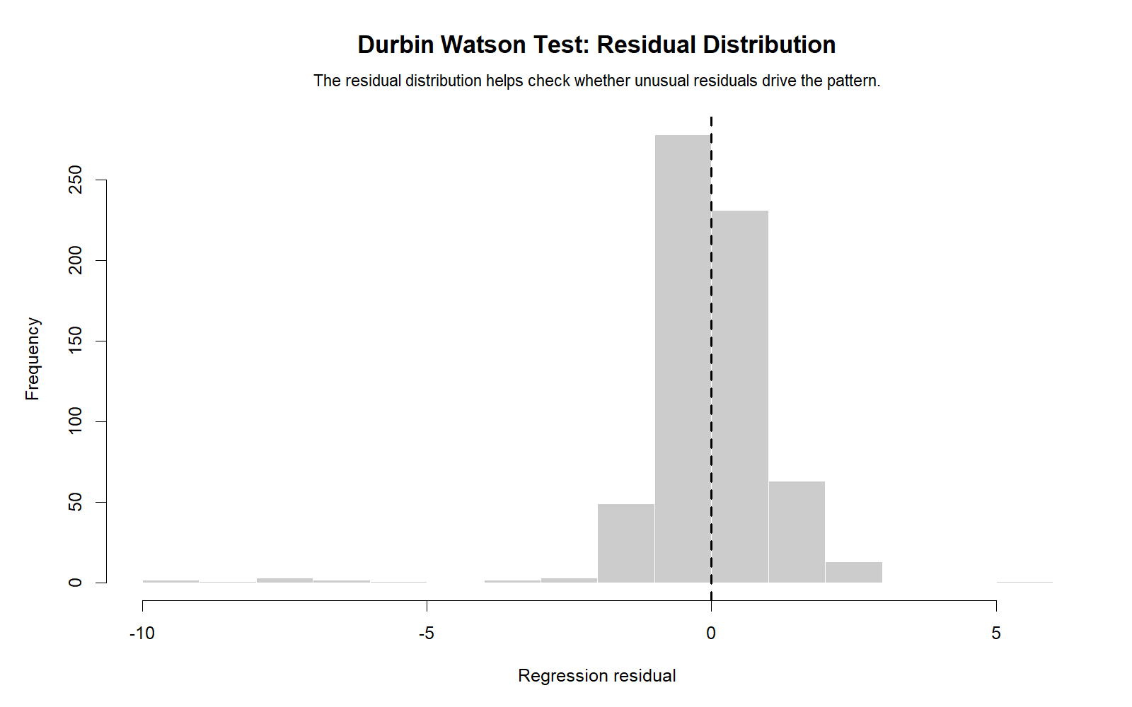
Detailed interpretation

The R residual histogram confirms that residuals are centered near zero but not perfectly normal. This agrees with the SPSS residual normality results, where both Kolmogorov-Smirnov and Shapiro-Wilk tests reject normality at p < .001.

Decision/reporting conclusion: R confirms that residual normality is a separate concern from residual autocorrelation. The Durbin-Watson result is acceptable, but residual distribution should still be reported.

R Chart 6: Durbin Watson Reference Distribution

Detailed interpretation

The R reference distribution confirms that the observed Durbin-Watson statistic is close to the no-autocorrelation value of 2. A value of 1.85735 is slightly below 2 but not far enough to suggest serious positive autocorrelation.

Decision/reporting conclusion: R validates the main decision: there is no serious first-order autocorrelation in the regression residuals.

R Chart 7: Residuals vs Fitted Values

Detailed interpretation

The residuals-versus-fitted chart checks whether residuals remain randomly scattered across predicted G3 values. This chart is not the Durbin-Watson statistic itself, but it helps detect model pattern, unequal variance or nonlinearity that may affect interpretation.

Decision/reporting conclusion: R confirms that Durbin-Watson should be reported as one part of a full regression diagnostic workflow, not as the only residual check.

SPSS, Python, R and Excel Workflows for Durbin Watson Test

SPSS Workflow

1. Open the cleaned dataset in SPSS.
2. Go to Analyze > Regression > Linear.
3. Place G3 in the dependent variable box.
4. Place G1, G2, studytime, failures and absences in the independent variables box.
5. Open Statistics and select Durbin-Watson if using the built-in option.
6. Save predicted values and residuals if you need manual residual diagnostics.
7. Compute lagged residuals and residual differences if you want a manual Durbin-Watson calculation.
8. Export the SPSS output PDF for reporting.

Python Workflow

1. Load the dataset with pandas.
2. Fit an OLS regression model using statsmodels.
3. Extract residuals and fitted values.
4. Calculate Durbin-Watson with statsmodels.stats.stattools.durbin_watson().
5. Create observed-versus-fitted, residual sequence, lag residual scatter, ACF, histogram and residuals-versus-fitted charts.
6. Report whether the statistic is close to 2.

R Workflow

1. Load the dataset with read.csv().
2. Fit the model using lm(G3 ~ G1 + G2 + studytime + failures + absences).
3. Extract residuals and fitted values.
4. Calculate Durbin-Watson using a package function or the manual formula.
5. Create residual diagnostic charts.
6. Compare R results with SPSS and Python outputs.

Excel Workflow

1. Fit a regression model using Excel Data Analysis ToolPak or imported predicted values.
2. Create a residual column: observed G3 minus fitted G3.
3. Create a lag residual column by shifting residuals down one row.
4. Create a residual difference column: current residual minus lag residual.
5. Square residuals and residual differences.
6. Compute Durbin-Watson as sum of squared residual differences divided by sum of squared residuals.

SPSS Syntax, Python Code, R Code and Excel Formulas

SPSS Syntax for Durbin Watson Test

* Durbin Watson Test in SPSS.
* Dependent variable: G3.
* Predictors: G1, G2, studytime, failures, absences.

SET PRINTBACK=OFF MPRINT=OFF.

TITLE "Durbin Watson Test Regression for G3".

REGRESSION
  /DEPENDENT G3
  /METHOD=ENTER G1 G2 studytime failures absences
  /STATISTICS COEFF OUTS R ANOVA CHANGE DW
  /SAVE PRED(pred_G3) RESID(resid_G3).

* Create sequential case id.
COMPUTE case_id = $CASENUM.
EXECUTE.

SORT CASES BY case_id.

* Create lag residual and residual difference.
CREATE lag_resid_G3 = LAG(resid_G3).
COMPUTE resid_diff_G3 = resid_G3 - lag_resid_G3.
COMPUTE sq_resid_G3 = resid_G3 ** 2.
COMPUTE sq_resid_diff_G3 = resid_diff_G3 ** 2.
EXECUTE.

* Manual Durbin-Watson components.
AGGREGATE
  /OUTFILE=* MODE=ADDVARIABLES
  /BREAK=
  /dw_n = N(resid_G3)
  /sum_sq_resid = SUM(sq_resid_G3)
  /sum_sq_resid_diff = SUM(sq_resid_diff_G3).

COMPUTE durbin_watson = sum_sq_resid_diff / sum_sq_resid.
COMPUTE approx_lag1_resid_corr = 1 - (durbin_watson / 2).
EXECUTE.

REPORT FORMAT=LIST AUTOMATIC ALIGN(CENTER)
  /VARIABLES=dw_n sum_sq_resid sum_sq_resid_diff durbin_watson approx_lag1_resid_corr
  /TITLE "Manual Durbin Watson Statistic".

DESCRIPTIVES VARIABLES=pred_G3 resid_G3 lag_resid_G3 resid_diff_G3
  /STATISTICS=MEAN STDDEV MIN MAX.

EXAMINE VARIABLES=resid_G3
  /PLOT BOXPLOT HISTOGRAM NPPLOT
  /STATISTICS DESCRIPTIVES
  /CINTERVAL 95
  /MISSING LISTWISE
  /NOTOTAL.

CORRELATIONS
  /VARIABLES=resid_G3 lag_resid_G3
  /PRINT=TWOTAIL NOSIG
  /MISSING=PAIRWISE.

OUTPUT EXPORT
  /CONTENTS EXPORT=VISIBLE
  /PDF DOCUMENTFILE="Durbin-Watson-Test-SPSS-Output.pdf".

Python Code for Durbin Watson Test

import pandas as pd
import numpy as np
import statsmodels.api as sm
from statsmodels.stats.stattools import durbin_watson
from scipy import stats

df = pd.read_csv("spss_ready_data.csv")

variables = ["G3", "G1", "G2", "studytime", "failures", "absences"]
data = df[variables].dropna().copy()

y = data["G3"]
X = data[["G1", "G2", "studytime", "failures", "absences"]]
X = sm.add_constant(X)

model = sm.OLS(y, X).fit()

fitted = model.fittedvalues
resid = model.resid

dw = durbin_watson(resid)
approx_lag1_corr = 1 - (dw / 2)

print(model.summary())
print("Durbin-Watson statistic:", dw)
print("Approximate lag-1 residual correlation:", approx_lag1_corr)

# Manual Durbin-Watson calculation
resid_diff = np.diff(resid)
manual_dw = np.sum(resid_diff ** 2) / np.sum(resid ** 2)
print("Manual Durbin-Watson:", manual_dw)

# Lag-1 residual correlation
current_resid = resid.iloc[1:].reset_index(drop=True)
lag_resid = resid.iloc[:-1].reset_index(drop=True)
r, p = stats.pearsonr(current_resid, lag_resid)

print("Lag-1 residual correlation:", r)
print("Lag-1 residual p-value:", p)

if 1.5 < dw < 2.5:
    print("No serious first-order autocorrelation indicated.")
elif dw <= 1.5:
    print("Possible positive autocorrelation.")
else:
    print("Possible negative autocorrelation.")

R Code for Durbin Watson Test

# Durbin Watson Test in R

df <- read.csv("spss_ready_data.csv")

data <- na.omit(df[, c("G3", "G1", "G2", "studytime", "failures", "absences")])

model <- lm(G3 ~ G1 + G2 + studytime + failures + absences, data = data)

summary(model)

resid_values <- residuals(model)
fitted_values <- fitted(model)

# Manual Durbin-Watson statistic
resid_diff <- diff(resid_values)
dw_manual <- sum(resid_diff^2) / sum(resid_values^2)
approx_lag1_corr <- 1 - (dw_manual / 2)

cat("Manual Durbin-Watson:", dw_manual, "\n")
cat("Approximate lag-1 residual correlation:", approx_lag1_corr, "\n")

# Lag residual correlation
current_resid <- resid_values[-1]
lag_resid <- resid_values[-length(resid_values)]
lag_cor <- cor.test(current_resid, lag_resid)

print(lag_cor)

# Optional package method
# install.packages("lmtest")
library(lmtest)
dwtest(model)

# Basic diagnostic plots
plot(fitted_values, resid_values,
     xlab = "Fitted values",
     ylab = "Residuals",
     main = "Residuals vs Fitted Values")
abline(h = 0, lty = 2)

plot(seq_along(resid_values), resid_values,
     xlab = "Observation order",
     ylab = "Residuals",
     main = "Residual Sequence Plot")
abline(h = 0, lty = 2)

hist(resid_values,
     main = "Residual Histogram",
     xlab = "Residuals")

acf(resid_values,
    main = "Residual Autocorrelation by Lag")

Excel Formulas for Durbin Watson Test

Assume:

A = observation order
B = observed G3
C = fitted G3
D = residual
E = lag residual
F = residual difference
G = squared residual
H = squared residual difference

Residual in D2:
=B2-C2

Lag residual in E3:
=D2

Residual difference in F3:
=D3-E3

Squared residual in G2:
=D2^2

Squared residual difference in H3:
=F3^2

Sum of squared residuals:
=SUM(G2:G650)

Sum of squared residual differences:
=SUM(H3:H650)

Durbin-Watson statistic:
=SUM(H3:H650)/SUM(G2:G650)

Approximate lag-1 residual correlation:
=1-(DurbinWatsonCell/2)

Interpretation:
DW near 2 = no serious autocorrelation.
DW below 2 = possible positive autocorrelation.
DW above 2 = possible negative autocorrelation.

APA Reporting Wording for Durbin Watson Test

When reporting the Durbin Watson Test, include the regression model, dependent variable, predictors, Durbin-Watson statistic and residual independence conclusion. If you also computed lag residual correlation, report it as supporting evidence.

APA-Style Report

Short Report Sentence

Careful Report Sentence for Cross-Sectional Data

Common Mistakes in Durbin Watson Test Interpretation

When to Use Durbin Watson Test

Use the Durbin Watson Test when you have a regression model and need to check whether residuals are autocorrelated across an ordered sequence. It is especially useful in time-series regression, ordered observations, repeated measurements, and models where the independence of errors is a key assumption.

For a full assumption-checking workflow, use Durbin-Watson with histogram interpretation, Q-Q plot normality check, box plot interpretation, coefficient of variation, central limit theorem, Goldfeld-Quandt test, and Ramsey RESET test.

Downloads and Resources for Durbin Watson Test

The resources below include the verified SPSS output PDF, Python charts and R validation charts used in this Salar Cafe Durbin Watson Test guide.

Related Internal Links for Salar Cafe Statistical Guides

Use these related Salar Cafe guides to connect the Durbin Watson Test with normality testing, regression diagnostics, variance tests, transformation methods, descriptive statistics, confidence intervals and reporting.