
SPSS T-Test Output, Assumptions, p-values and Reporting
T Test in SPSS: One Sample, Independent Samples and Paired Samples Output Guide
T Test in SPSS is used when you want to compare means and decide whether a mean difference is statistically significant. This guide is only about SPSS. It explains the one-sample t test, independent-samples t test and paired-samples t test using real SPSS output tables, assumption checks, Levene’s test, normality checks, p-values, confidence intervals, charts and ready-to-use reporting examples.
Quick Answer: T Test in SPSS Result
The SPSS output in this guide uses student grade variables. The main outcome is G3 final grade. The descriptive statistics show N = 649, mean G3 = 11.91, standard deviation = 3.231, and valid listwise cases = 649. The article then demonstrates three SPSS t-test procedures: one-sample t test, independent-samples t test and paired-samples t test.
The one-sample t test in SPSS compares the G3 mean with the reference value 10. SPSS reports t(648) = 15.030, Sig. (2-tailed) = .000, mean difference = 1.906, and 95% confidence interval [1.66, 2.16]. Because SPSS displays very small p-values as .000, the result should be reported as p < .001. The final grade mean is significantly higher than 10.
The independent-samples t test in SPSS compares female and male students on G3. Female students have a higher mean final grade, M = 12.25, than male students, M = 11.41. Levene’s test is not significant, p = .950, so the equal-variances-assumed row is used. SPSS reports t(647) = 3.311, p = .001, mean difference = .847, and 95% confidence interval [.345, 1.350]. The female group scored significantly higher on final grade.
The paired-samples t tests in SPSS compare grade periods from the same students. G1 vs G2 is significant, t(648) = -2.945, p = .003. G2 vs G3 is significant, t(648) = -6.695, p < .001. G1 vs G3 is also significant, t(648) = -7.093, p < .001. The negative signs occur because of the subtraction order in SPSS; practically, the later grade means are higher.
Final conclusion: The SPSS output shows that the final grade mean is significantly above 10, female students have a significantly higher final-grade mean than male students, and the same students show statistically significant grade increases from earlier grade periods to final grade.
Important SPSS rule: Do not report Sig. = .000 as p = .000. In SPSS write-up, report it as p < .001. Also, for independent-samples t tests, always check Levene’s Test for Equality of Variances before choosing which row to interpret.
Table of Contents
- What Is a T Test in SPSS?
- Which T Test Should You Use in SPSS?
- Internal Learning Path for SPSS T Test
- Dataset and Variables Used in the SPSS Output
- SPSS Descriptive Statistics Before T Testing
- SPSS T Test Assumptions and Normality Checks
- One-Sample T Test in SPSS
- Independent-Samples T Test in SPSS
- Paired-Samples T Test in SPSS
- SPSS Charts Used to Explain the T Test
- How to Run T Test in SPSS
- SPSS Syntax for T Tests
- How to Report T Test Results from SPSS
- Common Mistakes in SPSS T Test Interpretation
- Related Guides
- FAQs
What Is a T Test in SPSS?
A T Test in SPSS is a mean-comparison procedure. It helps answer whether a sample mean differs from a fixed value, whether two independent groups have different means, or whether two related measurements from the same cases differ from each other. SPSS produces standard output tables that make the result easy to report if you know which columns to read.
The most important SPSS output columns are t, df, Sig. (2-tailed), Mean Difference, Std. Error Difference and 95% Confidence Interval. The t statistic shows the size of the mean difference relative to sampling error. The degrees of freedom show the sample-size basis of the test. The p-value tells whether the result is statistically significant. The confidence interval gives the likely range of the true mean difference.
This SPSS guide should be read together with the wider Student’s t test guide if you need the basic theory, the t-test assumptions guide if you need assumption rules, and the effect size guide if you want to add practical importance after reporting statistical significance.
Simple definition: A t test in SPSS checks whether the observed mean difference is large enough, compared with its standard error, to be treated as statistically significant.
Which T Test Should You Use in SPSS?
SPSS has different t-test procedures because not every mean-comparison question has the same design. The correct procedure depends on whether you are comparing one mean to a benchmark, two separate groups, or two related measurements from the same cases.
| SPSS T Test Type | Use It When | Example in This Article | Related Salar Cafe Guide |
|---|---|---|---|
| One-sample t test | You compare one sample mean with a fixed reference value. | Test whether mean G3 differs from 10. | One Sample T Test |
| Independent-samples t test | You compare two separate groups. | Compare female and male students on G3. | Independent Samples T Test |
| Paired-samples t test | You compare two related measurements from the same cases. | Compare G1 vs G2, G2 vs G3, and G1 vs G3. | T Test for Difference Between Paired Means |
| Welch’s t test | You compare two groups but variances are not equal. | Use when Levene’s test is significant. | Welch’s T Test |
For independent-samples output, SPSS gives two rows: Equal variances assumed and Equal variances not assumed. If Levene’s test is not significant, use the equal-variances-assumed row. If Levene’s test is significant, use the unequal-variance row, which is related to the t test for unequal variances.
Internal Learning Path for SPSS T Test
Readers who arrive on this page often search for “how to run t test in SPSS” but also need help understanding the output. A strong learning path starts with mean, median and mode, standard deviation, standard error, and confidence interval. These concepts appear directly inside the SPSS output tables.
For assumptions, the most important supporting pages are t-test assumptions, normal distribution, Shapiro-Wilk test, Kolmogorov-Smirnov test, Q-Q plot normality check, histogram interpretation, and box plot interpretation. These guides explain why the SPSS Explore output is included before the t-test tables.
For reporting decisions, the reader should understand p-value, effect size, two-tailed t test, one-tailed t test, and the difference between a t test for equal variances and a t test for unequal variances. This internal path makes the SPSS output more useful than a simple screenshot-only tutorial.
Dataset and Variables Used in the SPSS Output
The SPSS output uses student grade variables. The main variables are G1, G2 and G3. G1 is the first-period grade, G2 is the second-period grade, and G3 is the final grade. The independent-samples example uses sex as the grouping variable, comparing female and male students. The paired-samples examples compare grade periods from the same students.
| Variable | SPSS Role | Used In | Interpretation |
|---|---|---|---|
| G1 | Scale variable | Paired-samples t test | First-period grade. |
| G2 | Scale variable | Paired-samples t test | Second-period grade. |
| G3 | Main scale outcome | One-sample and independent-samples t tests | Final grade. |
| sex | Grouping variable | Independent-samples t test | Female and male group comparison. |
SPSS Descriptive Statistics Before T Testing
Descriptive statistics should be checked before interpreting a t test. They show the sample size, mean, standard deviation, minimum and maximum values. This helps confirm that the variable is suitable for mean comparison and gives the reader a practical sense of the data before the p-value is discussed.
SPSS Descriptive Statistics for G1, G2, G3 and Absences
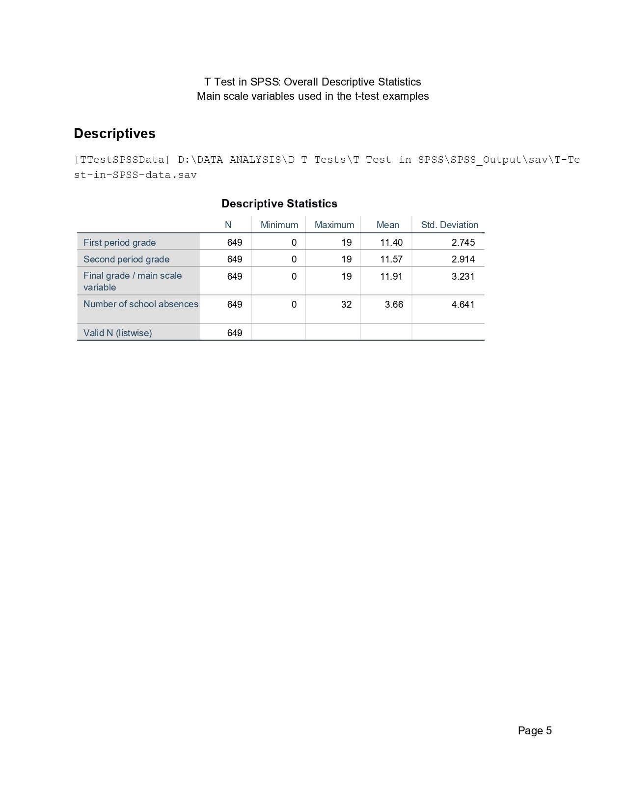
This SPSS table shows 649 valid cases for the main grade variables. The G3 final grade mean is 11.91, with a standard deviation of 3.231. This gives the foundation for the one-sample t test because the article later tests whether the G3 mean is significantly different from the reference value of 10.
The table also shows a gradual increase across the grade variables. G1 has a mean of about 11.40, G2 has a mean of about 11.57, and G3 has a mean of about 11.91. This pattern prepares the reader for the paired-samples t tests, where the same students are compared across time. The descriptive statistics do not prove significance by themselves, but they show the direction of the differences.
SPSS Descriptive Report by Sex
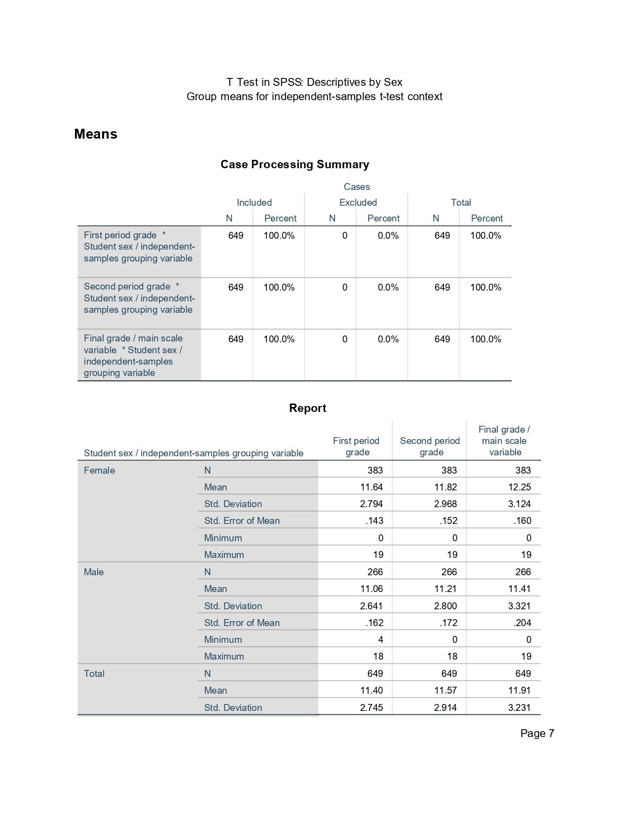
This SPSS output separates the grade variables by sex. It is useful before the independent-samples t test because it shows the group means and sample sizes. Female students have a higher G3 mean, about 12.25, while male students have a lower G3 mean, about 11.41. The female group also has more cases than the male group.
This figure should not be interpreted as the final test. It only shows the descriptive direction. The independent-samples t test is needed to decide whether the observed female-male mean difference is statistically significant after accounting for standard error and degrees of freedom. This is why the article later connects the descriptive table with Levene’s test and the Independent Samples Test table.
SPSS T Test Assumptions and Normality Checks
A t test in SPSS is strongest when the design matches the correct test and the assumptions are reasonably satisfied. For a one-sample t test, the outcome should be scale-like and the sample should be independent. For an independent-samples t test, the two groups should be independent and Levene’s test should be checked. For a paired-samples t test, the same cases should be measured twice and the difference scores should be checked.
| Assumption | Where to Check in SPSS | How to Interpret |
|---|---|---|
| Scale outcome | Variable View and descriptive output | The dependent variable should be numeric and suitable for mean comparison. |
| Independence | Study design | Independent-samples t test requires separate groups; paired-samples t test requires related measurements. |
| Normality context | Explore, Tests of Normality, Q-Q plots, histograms and boxplots | Large samples reduce concern, but strong outliers and severe non-normality should be reported. |
| Equality of variances | Levene’s Test in Independent Samples Test table | If p > .05, use equal variances assumed. If p < .05, use equal variances not assumed. |
SPSS Tests of Normality for G3 by Sex
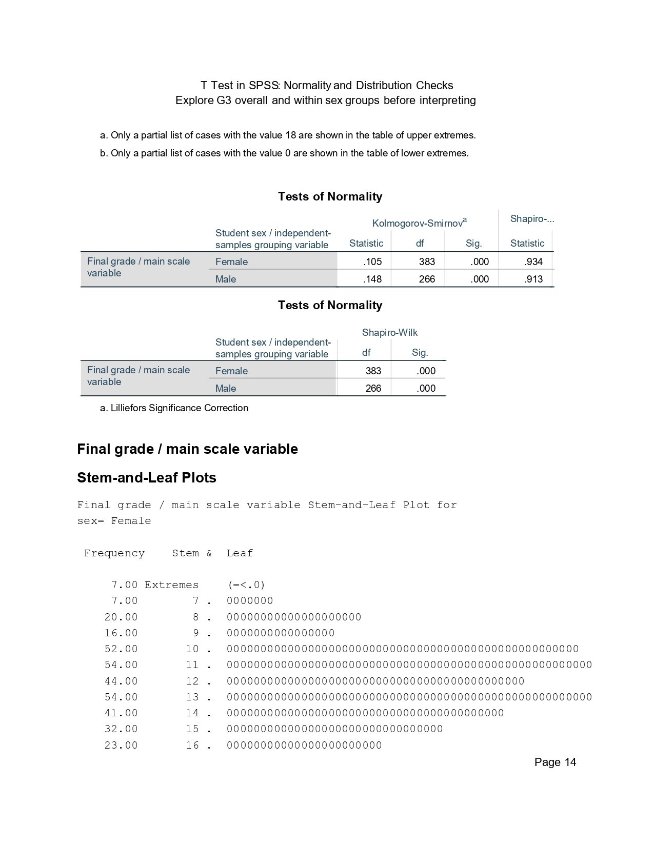
This SPSS table reports the Kolmogorov-Smirnov and Shapiro-Wilk normality tests for G3 separately by sex. The significance values are below .05, which means the distributions differ from a perfect normal distribution. This matches what is usually expected in grade data because grades are bounded and can include low-score outliers.
However, normality-test p-values can become significant very easily when the sample size is large. With hundreds of cases, even small departures from normality can produce significant Shapiro-Wilk or Kolmogorov-Smirnov results. Therefore, this output should not be used to automatically reject the t test. It should be interpreted together with the Q-Q plots, boxplots, histogram and sample size.
SPSS Normal Q-Q Plots for G3 by Sex
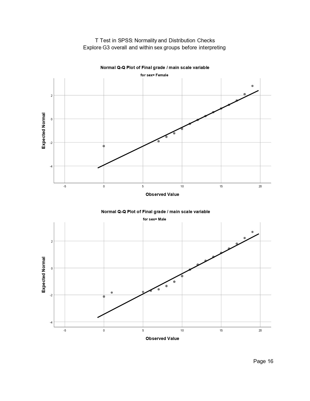
The Q-Q plots compare observed G3 values with the values expected under a normal distribution. Points close to the diagonal line support approximate normality. Points far from the line show where the distribution departs from normality. In this output, the middle of the distribution follows the line more closely than the lower tail.
This figure improves the assumption discussion because it shows the distribution visually rather than relying only on a normality-test p-value. The result is not perfect normality, but the central pattern is still readable, and the large sample size supports using the t test with a clear note about non-normal tails and outliers.
SPSS Boxplot and Detrended Q-Q Plot for G3 by Sex
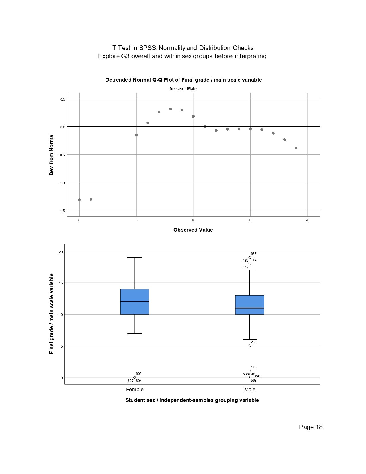
The boxplot is especially useful for the independent-samples t test because it compares the female and male distributions directly. The female group is visually higher than the male group, which agrees with the group means. The plot also shows low-score outliers, which explain why the normality tests are significant.
The detrended Q-Q plot highlights departures from the normal line by showing deviations around zero. Together, the boxplot and detrended plot show that the groups are not perfectly normal but still have clear central distributions. This is the correct type of chart to include because it explains the assumption context naturally and supports the later independent-samples interpretation.
One-Sample T Test in SPSS
A one-sample t test in SPSS compares one sample mean with a fixed reference value. In this output, the test checks whether the final grade mean, G3, differs from the reference value 10. This is useful when 10 represents a pass benchmark, expected value or research comparison point.
SPSS One-Sample T Test Output
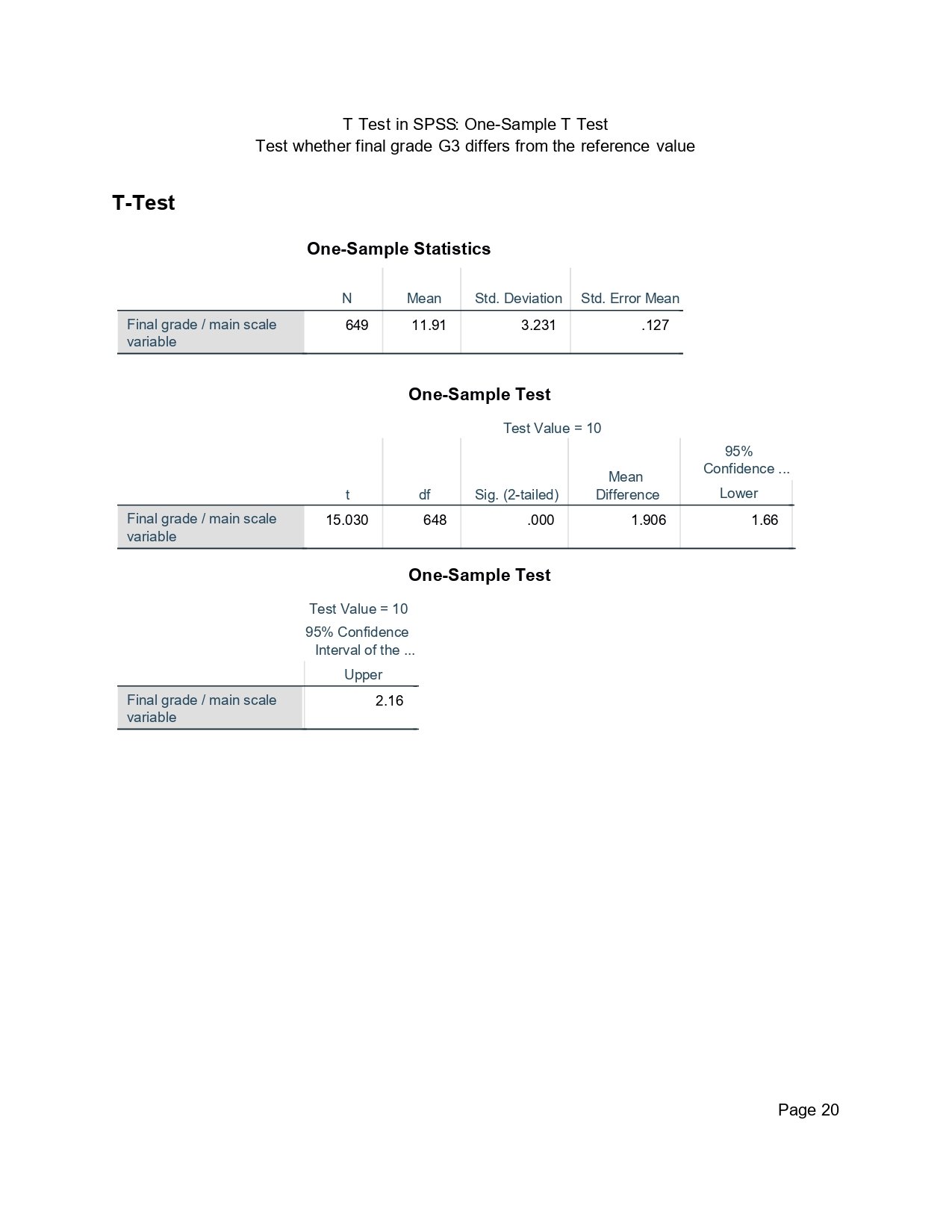
The One-Sample Statistics table shows N = 649, Mean = 11.91, Std. Deviation = 3.231, and Std. Error Mean = .127. The standard error tells how precisely the sample mean estimates the population mean. Because the sample is large, the standard error is much smaller than the standard deviation.
The One-Sample Test table reports t = 15.030, df = 648, Sig. (2-tailed) = .000, mean difference = 1.906, and 95% confidence interval [1.66, 2.16]. Since the p-value should be written as p < .001 and the confidence interval is entirely above zero, the G3 mean is significantly higher than 10.
One-sample SPSS conclusion: The final grade mean was significantly higher than the test value of 10, t(648) = 15.030, p < .001, mean difference = 1.906, 95% CI [1.66, 2.16].
Independent-Samples T Test in SPSS
An independent-samples t test in SPSS compares two separate groups. In this example, the two groups are female and male students, and the outcome is G3 final grade. This test is appropriate because each student belongs to only one sex group, so the groups are independent.
SPSS Independent-Samples T Test for G3 by Sex
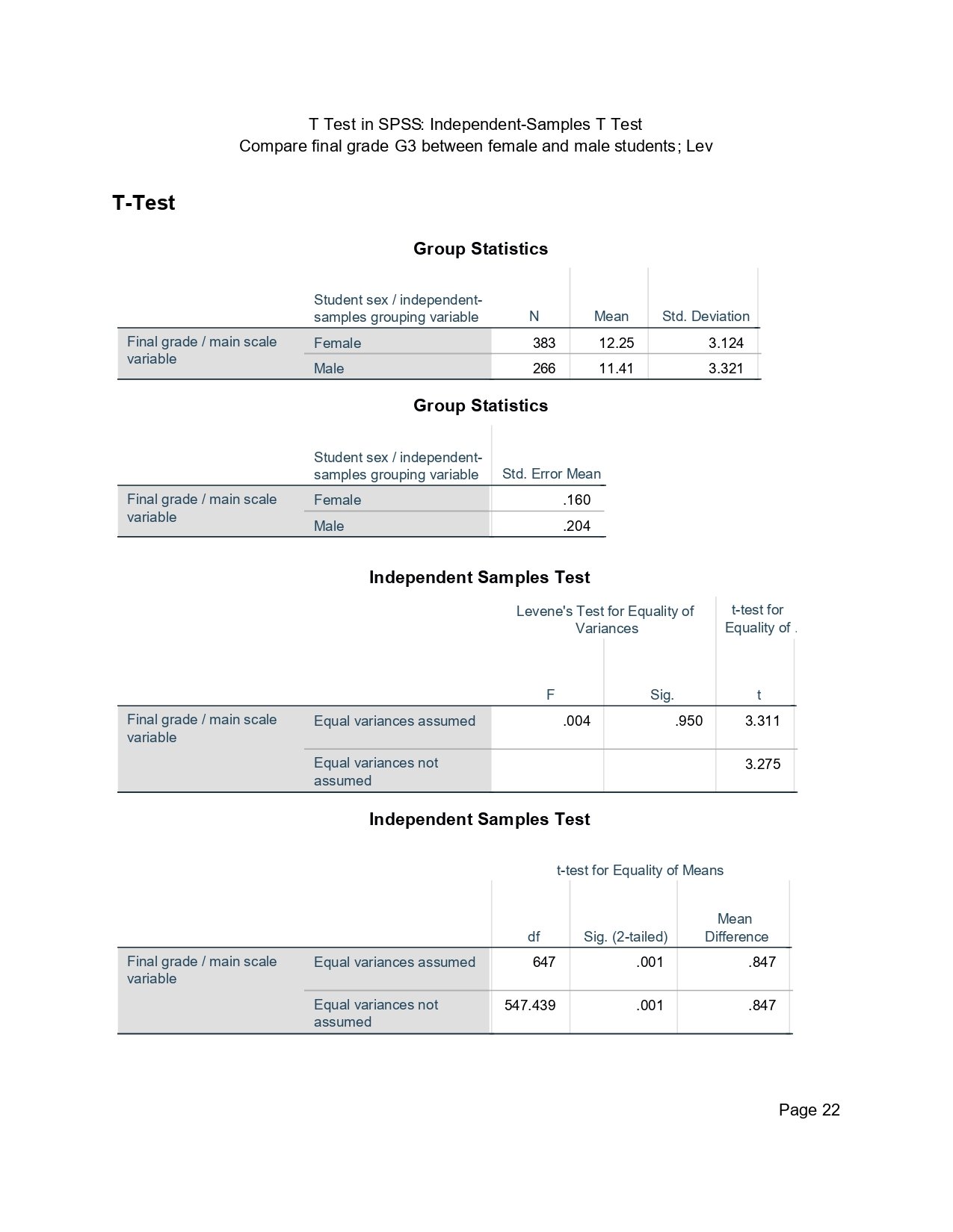
The Group Statistics table shows that female students have N = 383, Mean = 12.25, and SD = 3.124. Male students have N = 266, Mean = 11.41, and SD = 3.321. This descriptive result shows that the female group has the higher final-grade mean.
The Independent Samples Test table begins with Levene’s Test for Equality of Variances. Levene’s test has F = .004 and Sig. = .950. Since .950 is greater than .05, the equal-variances-assumed row is used. That row reports t(647) = 3.311 and p = .001, meaning the female-male difference in G3 is statistically significant.
SPSS Confidence Interval for the Independent-Samples T Test
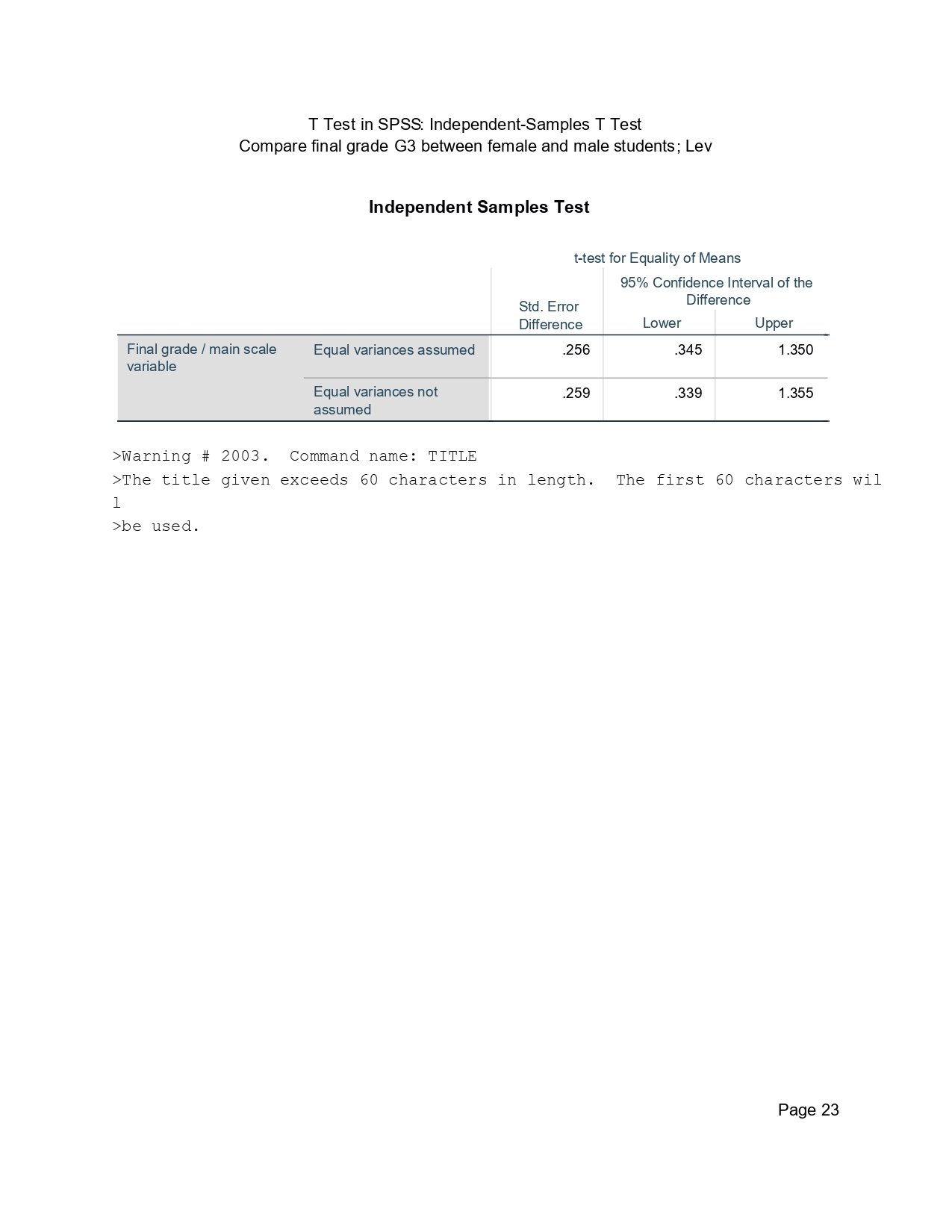
This output continues the independent-samples t-test table and shows the mean difference and confidence interval. The equal-variances-assumed row gives a mean difference of .847. The 95% confidence interval is approximately [.345, 1.350].
The confidence interval does not include zero, so it agrees with the p-value decision. The interpretation is not only that the result is significant, but also that the female group’s mean final grade is estimated to be about 0.85 grade points higher than the male group’s mean final grade. This is the part many weak competitor posts miss; a complete SPSS explanation should interpret both the p-value and the confidence interval.
Independent-samples SPSS conclusion: Female students had a significantly higher final-grade mean than male students, t(647) = 3.311, p = .001, mean difference = .847, 95% CI [.345, 1.350]. Levene’s test was not significant, so the equal-variances-assumed row was used.
SPSS Group Statistics for G1, G2 and G3 by Sex
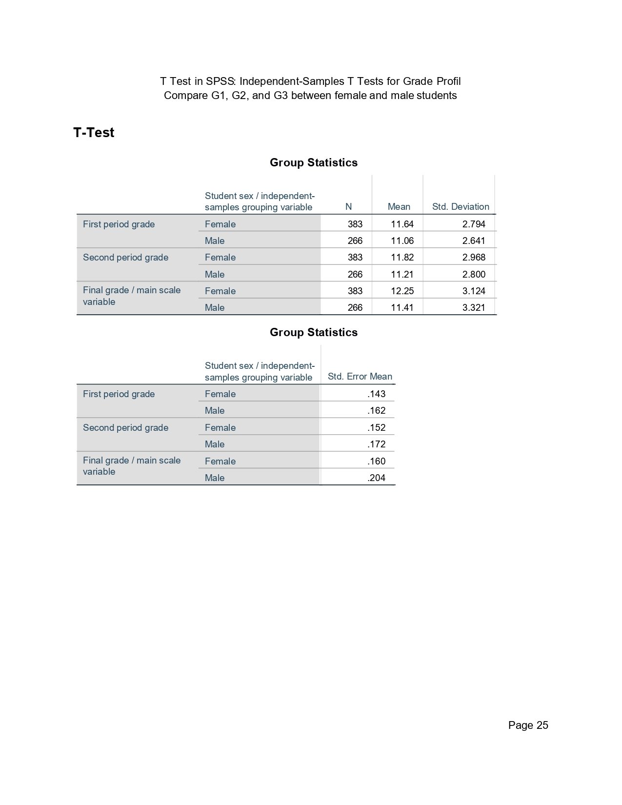
This table expands the independent-samples comparison across G1, G2 and G3. Female students have higher means on all three grade variables. This makes the result more informative because the final-grade difference is part of a consistent grade pattern rather than a single isolated comparison.
For G1, females average about 11.64 and males average about 11.06. For G2, females average about 11.82 and males average about 11.21. For G3, females average about 12.25 and males average about 11.41. The next output confirms whether these descriptive differences are statistically significant.
SPSS Independent-Samples Tests for G1, G2 and G3
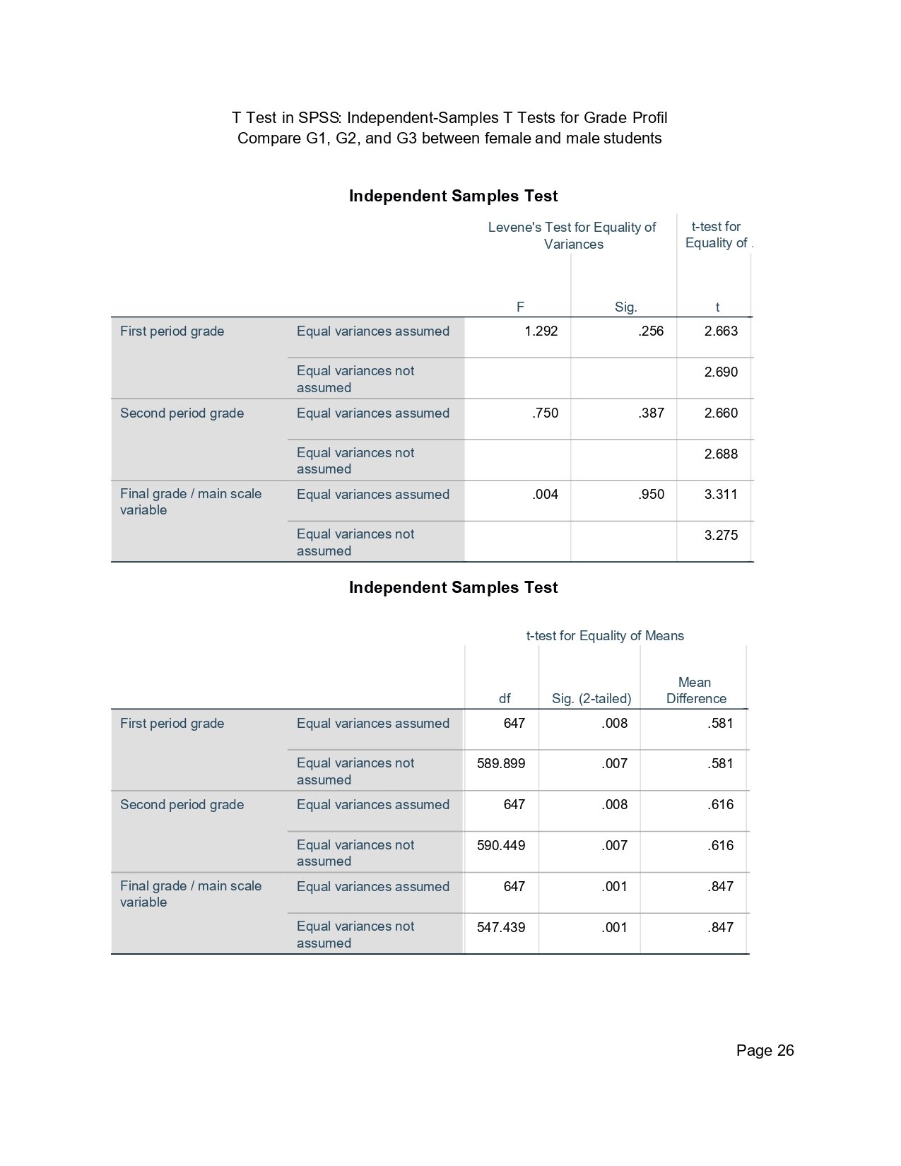
This table gives the inferential test results for the female-male differences across all three grade variables. The equal-variances-assumed row is used when Levene’s test is not significant. For G1 and G2, the p-values are about .008. For G3, the p-value is about .001.
The result shows that female students score significantly higher than male students across G1, G2 and G3. This is useful because it gives a stronger narrative than reporting only one final-grade t test. It shows that the group difference is visible across the grade sequence and strongest in the final grade comparison.
SPSS Confidence Intervals for G1, G2 and G3
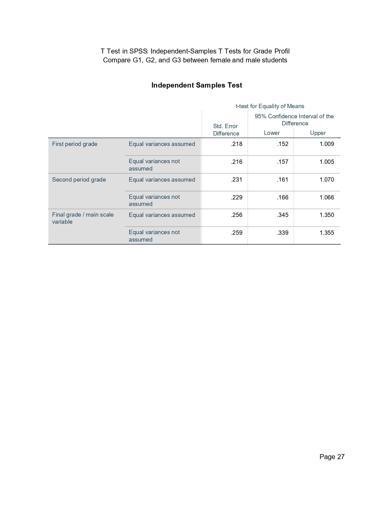
This image is necessary because it completes the independent-samples interpretation. It shows the confidence interval columns for G1, G2 and G3. The confidence intervals for the equal-variances-assumed rows are above zero, which confirms that the female-male differences are positive and statistically significant.
The G3 interval is especially important: approximately [.345, 1.350]. This tells the reader the likely size of the final-grade difference, not just whether it exists. A strong SPSS post should always explain the confidence interval because it is more informative than the p-value alone.
Paired-Samples T Test in SPSS
A paired-samples t test in SPSS compares two related measurements from the same cases. Here, the same students have grades at different periods: G1, G2 and G3. Because the same students appear in both measurements, this is not an independent-samples design. The correct SPSS procedure is paired-samples t test.
SPSS Normality Tests for Paired Difference Scores
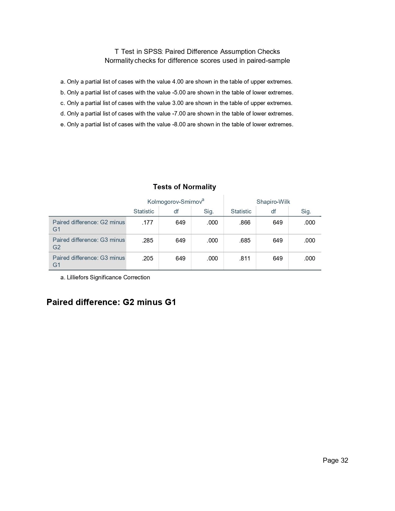
For paired-samples t testing, the normality assumption applies to the difference scores, not simply to each raw grade variable. This table checks the difference scores: G2 minus G1, G3 minus G2 and G3 minus G1. The normality tests are significant, which means the difference-score distributions are not perfectly normal.
This output is useful because it shows the correct assumption check for paired t tests. With a large sample of 649 students, the paired t test can still provide useful evidence, but the article should mention that the difference-score distributions include departures from perfect normality. This is why the next visual diagnostic is included.
SPSS Boxplot for G3 Minus G1 Difference Score
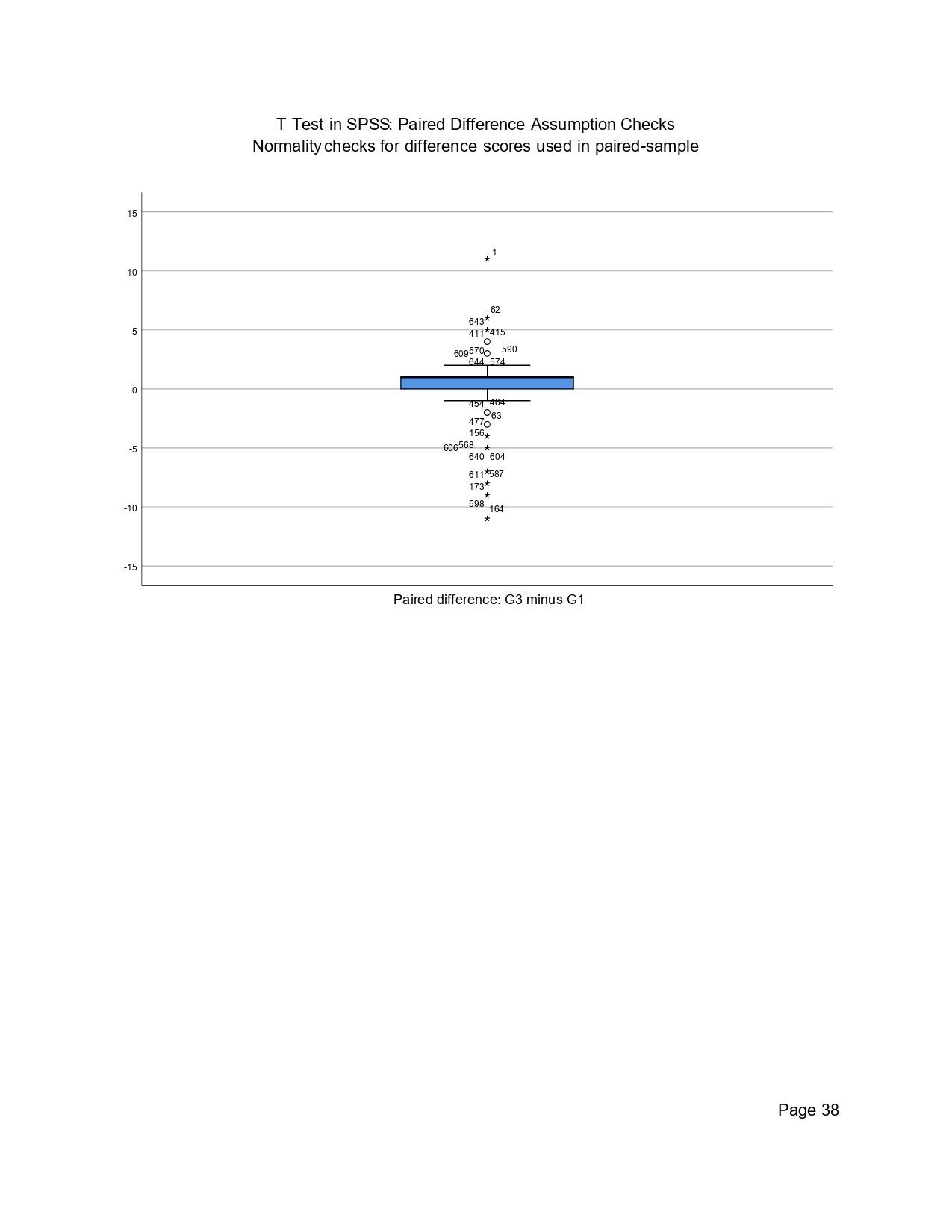
This boxplot shows the distribution of the total grade-change score from G1 to G3. Most students fall in the central part of the distribution, but there are also outlying changes. These outliers explain why the normality tests for paired differences are significant.
This chart is included because it is the most useful paired-difference visual for the article. It shows the full change from first-period grade to final grade, which is the largest paired comparison. Repeating every Q-Q plot and every extreme-value table would make the article heavy without improving the explanation, so this focused boxplot is enough for the main paired-difference diagnostic.
SPSS Paired-Samples T Test for G1 and G2
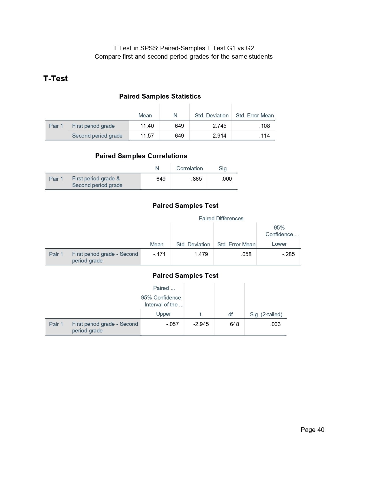
This SPSS output compares G1 and G2 for the same students. The Paired Samples Statistics table shows the two means, and the Paired Samples Correlations table shows that G1 and G2 are strongly related. A strong correlation is expected because students who perform well early usually perform well in the next grade period too.
The Paired Samples Test table reports t(648) = -2.945 and p = .003. The result is statistically significant. The mean difference is negative because SPSS subtracts G2 from G1 based on the variable order. Practically, this means G2 is significantly higher than G1.
SPSS Paired-Samples T Test for G2 and G3
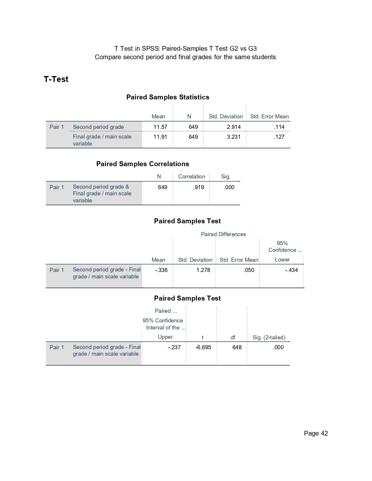
This output compares G2 and G3 for the same students. The final grade mean is higher than the second-period grade mean. The paired correlation is very strong, showing that students’ second-period grades and final grades are closely connected.
SPSS reports t(648) = -6.695 with p < .001. The result is statistically significant. Again, the negative sign is caused by SPSS subtraction order. The practical interpretation is that final grade is significantly higher than second-period grade.
SPSS Paired-Samples T Test for G1 and G3
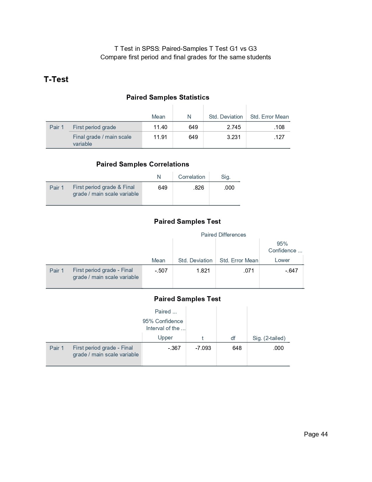
This SPSS output compares G1 and G3, which is the largest time-span comparison in the paired section. The final grade mean is higher than the first-period grade mean. The paired correlation is strong, meaning early performance and final performance are related.
SPSS reports t(648) = -7.093 with p < .001. This is the strongest paired-samples result in the article. The practical interpretation is that the final grade is significantly higher than the first-period grade. The negative sign should be explained in the write-up because it depends on the order in which SPSS subtracts the variables.
Paired-samples SPSS conclusion: The paired-samples t tests show significant grade increases from G1 to G2, from G2 to G3, and from G1 to G3. The largest change is between G1 and G3.
SPSS Charts Used to Explain the T Test
SPSS charts should be added only when they help explain the t test. This article includes three natural charts: a histogram for the distribution of G3, a mean line plot for the female-male comparison, and a scatterplot for the relationship between G1 and G3. These visuals support the tables without repeating unnecessary output pages.
SPSS Histogram of G3 Final Grade
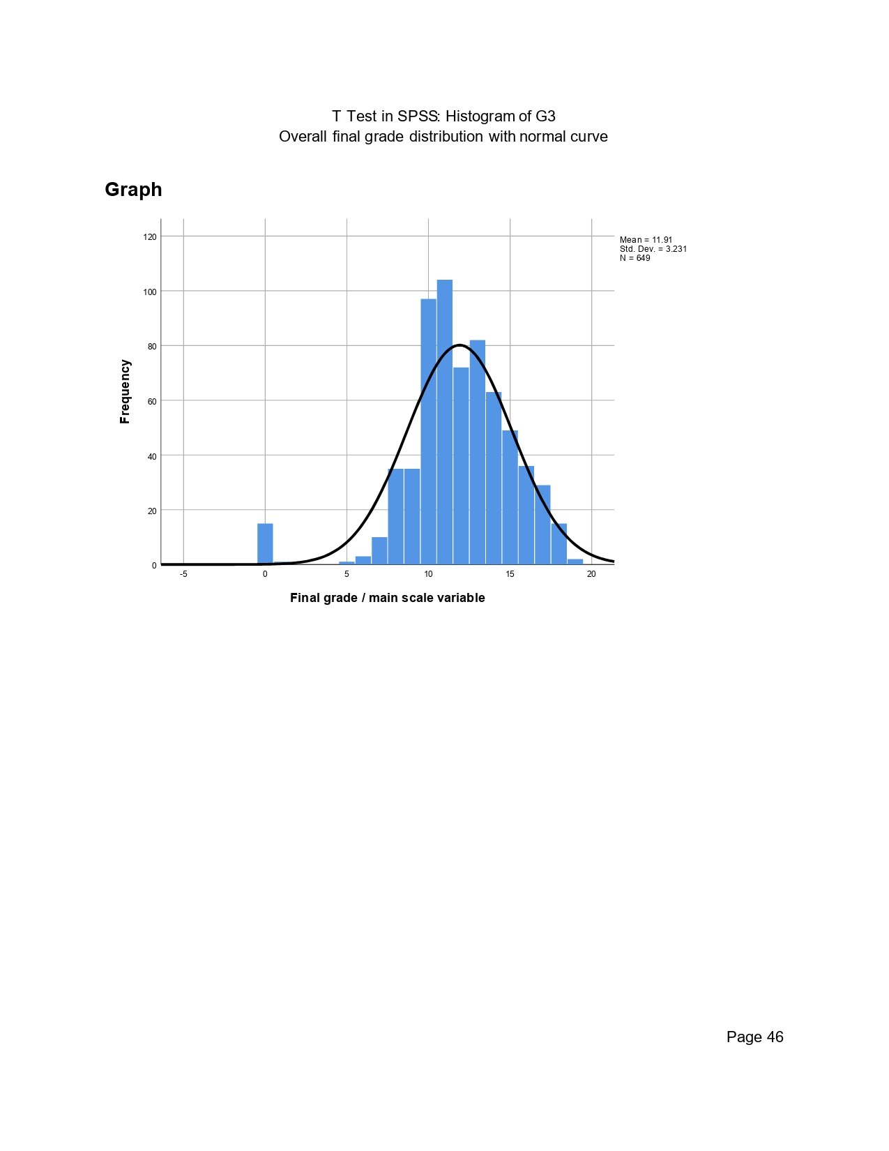
The histogram shows the shape of the G3 final-grade distribution. Most values are concentrated around the middle of the score range, and the mean is about 11.91. The normal curve overlay helps compare the observed grade distribution with a bell-shaped reference distribution.
The chart also shows low-score values that pull the distribution away from perfect normality. This matches the significant normality tests and Q-Q plot departures. The histogram is necessary because it gives readers a visual explanation of why assumption checking matters before reporting the t-test result.
SPSS Mean Line Plot of G3 by Sex
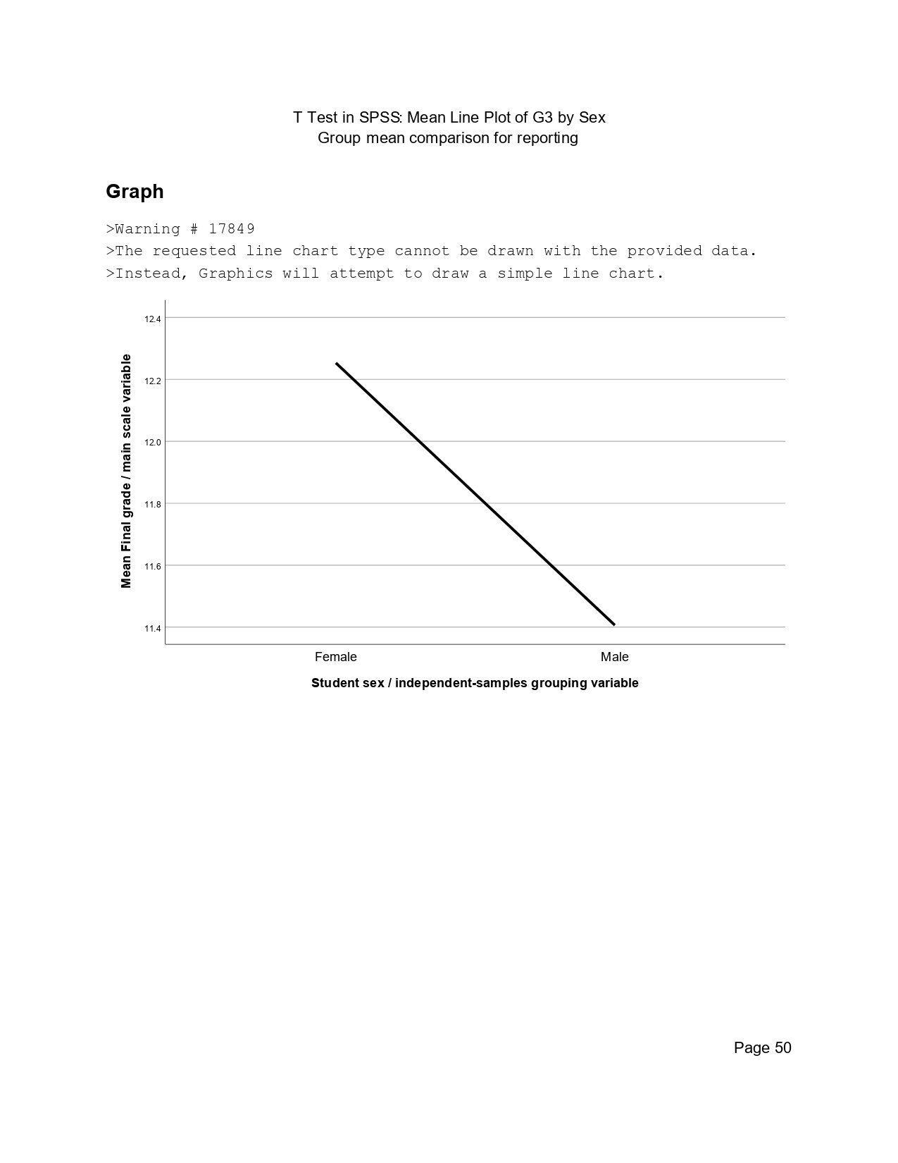
The mean line plot visually summarizes the independent-samples t test. The female mean is higher than the male mean, matching the Group Statistics table. This makes the direction of the result easy to understand before the reader studies the t statistic and p-value.
This chart is useful because it directly supports the independent-samples conclusion. It should not replace the t-test table, because the chart alone does not show Levene’s test, t, degrees of freedom or confidence interval. It works best as a visual companion to the SPSS Independent Samples Test output.
SPSS Scatterplot of G1 and G3
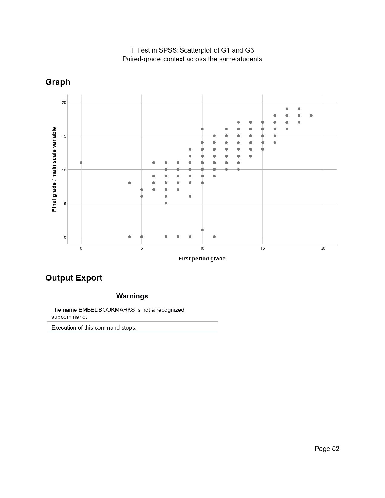
The scatterplot shows a strong positive relationship between G1 and G3. Students with higher first-period grades generally have higher final grades. This supports the paired-samples section because the same students’ grade measures are related across time.
This chart is not a t test by itself. It is included because it helps explain why paired-samples output often includes paired correlations. The t test checks whether the mean change is significant, while the scatterplot shows how closely the two related grade measures move together.
How to Run T Test in SPSS
How to Run One-Sample T Test in SPSS
- Open the dataset in SPSS.
- Go to Analyze > Compare Means > One-Sample T Test.
- Move G3 into the Test Variable(s) box.
- Enter the test value, such as 10.
- Click OK.
- Interpret One-Sample Statistics and One-Sample Test.
How to Run Independent-Samples T Test in SPSS
- Go to Analyze > Compare Means > Independent-Samples T Test.
- Move G3 into the Test Variable(s) box.
- Move sex into the Grouping Variable box.
- Click Define Groups and enter the two group codes used in your dataset.
- Click OK.
- Check Levene’s test first, then read the correct t-test row.
How to Run Paired-Samples T Test in SPSS
- Go to Analyze > Compare Means > Paired-Samples T Test.
- Select the related variables, such as G1 and G2.
- Move them into the Paired Variables box.
- Repeat for G2 with G3 and G1 with G3 if needed.
- Click OK.
- Interpret Paired Samples Statistics, Paired Samples Correlations and Paired Samples Test.
SPSS Syntax for T Tests
SPSS syntax helps users repeat the same analysis and avoid menu mistakes. The syntax below is SPSS-only and matches the procedures explained in this post.
One-Sample T Test Syntax
T-TEST
  /TESTVAL = 10
  /MISSING = ANALYSIS
  /VARIABLES = G3
  /CRITERIA = CI(.95).
Independent-Samples T Test Syntax
T-TEST GROUPS = sex(1 2)
  /MISSING = ANALYSIS
  /VARIABLES = G1 G2 G3
  /CRITERIA = CI(.95).
Paired-Samples T Test Syntax
T-TEST PAIRS = G1 WITH G2 (PAIRED)
  /CRITERIA = CI(.95)
  /MISSING = ANALYSIS.

T-TEST PAIRS = G2 WITH G3 (PAIRED)
  /CRITERIA = CI(.95)
  /MISSING = ANALYSIS.

T-TEST PAIRS = G1 WITH G3 (PAIRED)
  /CRITERIA = CI(.95)
  /MISSING = ANALYSIS.
SPSS Output Export Syntax
OUTPUT EXPORT
  /CONTENTS EXPORT=ALL
  /PDF DOCUMENTFILE='T-Test-in-SPSS-Output.pdf'.
How to Report T Test Results from SPSS
A strong SPSS t-test report should include the test type, group or variable names, means, standard deviations, t statistic, degrees of freedom, p-value, mean difference and confidence interval. If the test is independent-samples, also mention Levene’s test and which row was used.
One-Sample T Test Reporting Example
A one-sample t test showed that the final grade mean was significantly higher than the reference value of 10, t(648) = 15.030, p < .001. The mean difference was 1.906, with a 95% confidence interval from 1.66 to 2.16.
Independent-Samples T Test Reporting Example
An independent-samples t test compared final grade scores for female and male students. Levene’s test was not significant, p = .950, so the equal-variances-assumed row was used. Female students had a higher final-grade mean (M = 12.25, SD = 3.124) than male students (M = 11.41, SD = 3.321). The difference was statistically significant, t(647) = 3.311, p = .001, mean difference = .847, 95% CI [.345, 1.350].
Paired-Samples T Test Reporting Example
A paired-samples t test showed that final grade was significantly higher than first-period grade. The mean increased from 11.40 to 11.91. SPSS reported t(648) = -7.093, p < .001, with a paired mean difference of -.507 for G1 minus G3, 95% CI [-.647, -.367]. The negative sign reflects the SPSS subtraction order.
Common Mistakes in SPSS T Test Interpretation
| Mistake | Why It Is Wrong | Correct SPSS Practice |
|---|---|---|
| Using independent-samples t test for the same students measured twice | The observations are related, not independent. | Use paired-samples t test. |
| Ignoring Levene’s test | You may read the wrong row in the Independent Samples Test table. | Use equal variances assumed when Levene p > .05 and equal variances not assumed when Levene p < .05. |
| Reporting Sig. .000 as p = .000 | The p-value is not exactly zero. | Report p < .001. |
| Reporting only the p-value | The reader cannot see direction or size of the difference. | Report means, mean difference and 95% confidence interval. |
| Misreading the negative sign in paired output | SPSS subtracts variables in the order entered. | Explain the variable order and then state the practical direction. |
| Adding every SPSS screenshot without purpose | Too many repeated charts make the post difficult to read. | Use only screenshots that explain the result, assumption or reporting decision. |
FAQs About T Test in SPSS
What is a T Test in SPSS?
A T Test in SPSS is a mean-comparison procedure. It can compare one sample mean with a fixed value, two independent group means, or two related measurements from the same cases.
Which t test should I use in SPSS?
Use one-sample t test for one mean versus a reference value, independent-samples t test for two separate groups, and paired-samples t test for two related measurements from the same cases.
What does Sig. (2-tailed) mean in SPSS?
Sig. (2-tailed) is the two-tailed p-value. If it is below .05, the mean difference is usually considered statistically significant at the 5% level.
What does Levene’s test mean in SPSS t test output?
Levene’s test checks whether the two group variances are equal in an independent-samples t test. If Levene’s p-value is greater than .05, use the equal-variances-assumed row. If it is below .05, use the equal-variances-not-assumed row.
How do I report .000 in SPSS?
SPSS displays very small p-values as .000. Do not report p = .000. Report it as p < .001.
Why is the paired-samples t test result negative in SPSS?
The sign depends on the order of subtraction. If SPSS subtracts the later grade from the earlier grade and the later grade is higher, the mean difference and t value can be negative. Interpret the sign according to the variable order.
Do I need normality before running a t test in SPSS?
You should check normality context using Explore, Q-Q plots, histograms and boxplots. With large samples, t tests are often robust, but strong outliers and severe non-normality should be mentioned.

