Regression Diagnostics and Influential Case Detection
Influence Diagnostics are regression checking methods used to identify observations that may strongly affect fitted values, residuals, regression coefficients, standard errors or the final interpretation of a model. This complete guide explains Cook’s Distance, leverage, studentized residuals, DFFITS, DFBETAS and COVRATIO with SPSS, R, Python and Excel workflows using a G3 final-grade regression example.
Google AdSense top placement reserved here
Quick Answer: Influence Diagnostics Result
Influence Diagnostics were applied to a regression model predicting G3 final grade from G1, G2, studytime, failures, absences, age, Medu and Fedu. The model used 649 complete cases. The model fit was strong, but the diagnostic graphs showed that a small set of cases had unusually strong impact on the regression model.
Final result: The regression model predicted G3 strongly, R² = .851 and adjusted R² = .849. However, Influence Diagnostics identified several cases that require case-level review. Case 164 was the strongest influential case, with actual G3 = 0, fitted G3 ≈ 9.05, residual ≈ -9.05, Cook’s Distance ≈ .1468 and studentized residual ≈ -7.61. Other important review cases included 640, 587, 641, 627, 638, 173 and 520.
Important reporting note: Influence Diagnostics do not automatically prove that a case is wrong. They show which cases may have unusual influence. The correct action is to verify those rows in the original data, check whether they are valid observations, and then run a sensitivity analysis before deciding whether to keep, recode or exclude them.
What Are Influence Diagnostics?
Influence Diagnostics are statistical tools used after fitting a regression model to identify observations that may have unusual impact on model results. In ordinary least squares regression, each observation contributes to the fitted equation. Most observations have small influence. A few observations may pull the regression line, change coefficients, change fitted values, affect standard errors or create unusual residual patterns.
An influential case is not always a mistake. It may be a valid but unusual observation. In a student-performance dataset, a student may have strong previous grades but a final grade of zero because of absence, withdrawal, illness, final-exam failure or another factor not fully captured by the predictors. Such a case may strongly affect regression output, but it may still be real and meaningful.
Influence Diagnostics are different from ordinary outlier detection. A simple outlier has an unusual value. An influential case changes the model. Some outliers do not influence the model much. Some high-leverage observations are not residual outliers. The most important cases are those that combine unusual predictor patterns, large residuals and measurable model impact.
Practical note: Influence Diagnostics should be part of a complete regression workflow. They should be used together with residual plots, heteroscedasticity checks, normality checks and subject-matter interpretation. For related assumption testing, also see the Brown-Forsythe Test, Cochran C Test, Hartley F Max Test and Goldfeld-Quandt Test.
If you are building a complete data-analysis learning path, compare this regression guide with the DAgostino Pearson Test for normality, the Cramer von Mises Test for distribution checking and the Greenhouse-Geisser Correction for repeated-measures ANOVA correction.
Influence Diagnostics Formula and Main Measures
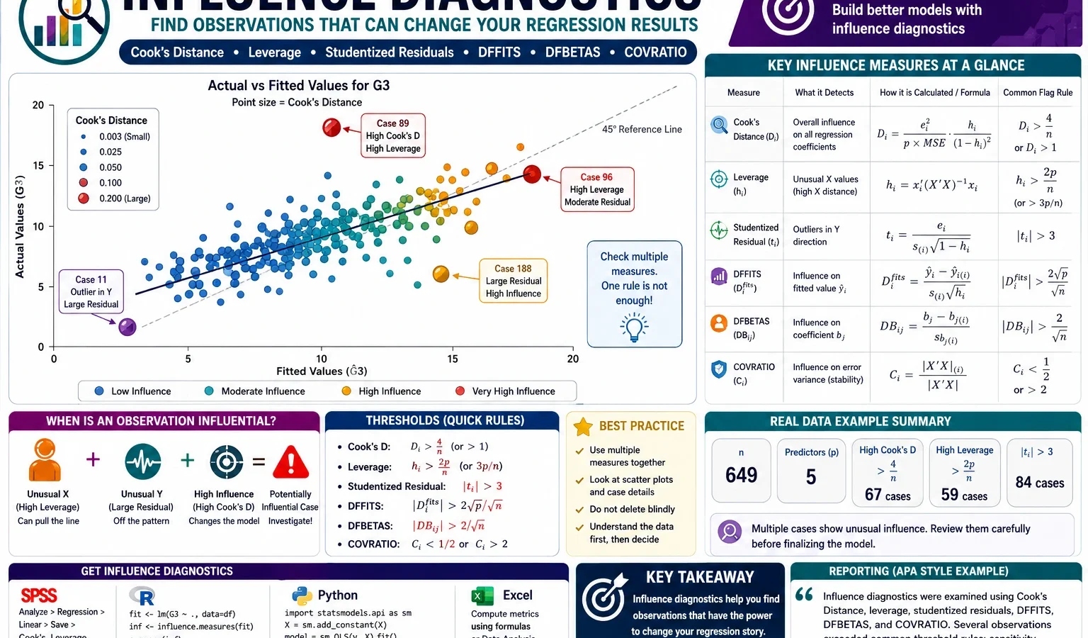
Influence Diagnostics are not one single statistic. They are a group of related measures. The most common measures are Cook’s Distance, leverage, studentized residuals, DFFITS, DFBETAS and COVRATIO. Each diagnostic answers a different question about case influence.
Cook’s Distance Formula
Cook’s Distance measures how much the fitted regression model changes when a case is removed. A common form of Cook’s Distance is:
D_i = (e_i² / p × MSE) × (h_i / (1 - h_i)²)In this formula, e_i is the residual for case i, p is the number of model parameters including the intercept, MSE is mean squared error and h_i is leverage. Cook’s Distance becomes large when a case has a large residual, high leverage or both.
Leverage Formula
Leverage is the diagonal value of the hat matrix. It measures how unusual a case is in the predictor space.
h_i = x_i' (X'X)^-1 x_iHigh leverage means that the predictor values of a case are unusual compared with other cases. A high-leverage case is not automatically harmful. It becomes more serious when it also has a large residual, high Cook’s Distance, high DFFITS or strong DFBETAS.
DFFITS, DFBETAS and COVRATIO
DFFITS measures how much a case changes its own fitted value. DFBETAS measure how much a case changes each regression coefficient. COVRATIO measures whether a case affects the covariance matrix and therefore the precision of regression estimates.
| Diagnostic | Common rule of thumb | Meaning | How it is used in this post |
|---|---|---|---|
| Cook’s Distance | D > 4/n or D > 4/(n-p) | Case may influence the overall fitted model. | Used to rank the strongest review cases, especially case 164. |
| Leverage | h > 2p/n or h > 3p/n | Case has an unusual predictor pattern. | Used to identify cases whose predictor values are far from the predictor center. |
| Studentized residual | |r| > 2 or |r| > 3 | Case has an unusually large prediction error. | Used to identify cases where actual G3 is much lower or higher than predicted. |
| DFFITS | |DFFITS| > 2√(p/n) | Case strongly affects fitted value prediction. | Used to detect cases that change predicted G3 values strongly. |
| DFBETAS | |DFBETAS| > 2/√n | Case strongly affects one or more coefficients. | Used to identify which coefficient is most affected by each case. |
| COVRATIO | Outside 1 ± 3p/n | Case may affect estimate precision and standard errors. | Used to check whether influential cases affect uncertainty in the model. |
Influence Diagnostics Null Hypothesis and Practical Question
Influence Diagnostics are usually not reported as a single hypothesis test like ANOVA or t-test. They are model-diagnostic checks. However, they still answer a clear practical question: Are any cases unusually influential in the regression model?
| Diagnostic question | Meaning | Applied to this example |
|---|---|---|
| Expected situation | No single case should strongly control the regression model. | Most students should have small Cook’s Distance, moderate leverage and reasonable residuals. |
| Diagnostic warning | Some cases may strongly affect fitted values, coefficients or standard errors. | Cases such as 164, 640, 587, 641, 627, 638, 173 and 520 require review. |
| Research decision | Flagged cases must be verified and tested through sensitivity analysis. | The model should be reported with diagnostic transparency, not automatic deletion. |
Because several diagnostics repeatedly identify the same observations, the correct conclusion is that the regression model is strong overall but contains case-level observations that deserve careful review.
Google AdSense middle placement reserved here
Dataset and Regression Model Used
This worked example uses the student performance dataset. The dependent variable is G3 final grade. The predictors are G1, G2, studytime, failures, absences, age, Medu and Fedu. The goal is to predict G3 and then check whether any cases strongly influence the fitted regression model.
| Item | Verified value | Explanation |
|---|---|---|
| Rows used | 649 | Total complete observations used in the model. |
| Dependent variable | G3 | Final grade predicted by the regression model. |
| Predictors | G1, G2, studytime, failures, absences, age, Medu, Fedu | Prior grades, study pattern, academic history, absences, age and parental education. |
| Model parameters | 9 | Eight predictors plus intercept. |
| Main method | Ordinary least squares regression | Used to estimate fitted G3 and diagnostic values. |
| Main diagnostics | Cook’s Distance, leverage, studentized residuals, DFFITS, DFBETAS, COVRATIO | Used to identify influential cases. |
External dataset source: UCI Machine Learning Repository: Student Performance dataset.
Regression Model
G3 = b0 + b1(G1) + b2(G2) + b3(studytime) + b4(failures)
     + b5(absences) + b6(age) + b7(Medu) + b8(Fedu) + error
The model is useful because G1 and G2 are strongly related to G3, while studytime, failures, absences, age and parental education provide additional explanatory information. However, a strong R-squared is not enough. Influence Diagnostics are needed to check whether selected rows are controlling part of the model behaviour.
Verified Influence Diagnostics Results in SPSS, R and Python
The analysis was reproduced with SPSS, R and Python. SPSS produced regression output and saved diagnostic variables. R and Python verified the same logic and created publication-ready charts. The overall model is strong, but several cases cross multiple diagnostic thresholds.
Model Fit Summary
| Statistic | Verified value | Interpretation |
|---|---|---|
| Number of cases | 649 | Complete cases included in the regression model. |
| R-squared | 0.850777 | The model explains about 85.1% of variation in G3. |
| Adjusted R-squared | 0.848912 | Adjusted fit remains very high after accounting for predictors. |
| Residual standard error | 1.255758 | Typical prediction error is about 1.26 grade points. |
| F statistic | 456.111097 | The overall regression model is highly significant. |
| Model p-value | 1.4549e-258 | Report as p < .001. |
The model fit summary shows that G3 is predicted very well overall. This is expected because G1 and G2 are previous grade measures and have a strong relationship with the final grade. However, Influence Diagnostics ask a different question. They do not ask whether the model is strong. They ask whether specific observations are unusually controlling the model.
Diagnostic Thresholds Used
| Diagnostic threshold | Verified value | Meaning |
|---|---|---|
| Cook’s Distance 4/n | 0.006163 | Candidate influence threshold. |
| Cook’s Distance 4/(n-p) | 0.006250 | Alternative Cook’s Distance threshold. |
| Leverage 2p/n | 0.027735 | Moderate leverage warning threshold. |
| Leverage 3p/n | 0.041602 | Stronger leverage warning threshold. |
| DFFITS threshold | 0.235521 | Case may strongly affect fitted prediction. |
| DFBETAS threshold | 0.078507 | Case may strongly affect one coefficient. |
| COVRATIO lower | 0.958398 | Lower precision-impact boundary. |
| COVRATIO upper | 1.041602 | Upper precision-impact boundary. |
These thresholds are screening cutoffs. They should not be treated as automatic deletion rules. In this example, the Cook’s Distance threshold is very small because the sample size is large. Therefore, any case above 0.0062 is marked for review, but cases far above this value deserve more attention than cases only slightly above it.
Case-Based Review Summary
| Case | Actual G3 | Fitted G3 | Residual | Cook’s Distance | Studentized residual | Case-based explanation |
|---|---|---|---|---|---|---|
| 164 | 0 | 9.050797 | -9.050797 | 0.146811 | -7.614187 | The model expected a moderate final grade, but the observed final grade was zero. This is the strongest case because it combines a very large negative residual with very high Cook’s Distance. |
| 640 | 0 | 7.563657 | -7.563657 | 0.088454 | -6.266918 | The model predicted a positive G3, but actual G3 was zero. It is the second strongest case by Cook’s Distance and is visible in several diagnostic charts. |
| 587 | 0 | 8.167641 | -8.167641 | 0.069273 | -6.777291 | This case has one of the largest negative prediction errors and appears strongly in Cook’s Distance, residual and DFFITS charts. |
| 641 | 0 | 6.830129 | -6.830129 | 0.063480 | -5.620008 | This case is influential because the final grade is much lower than the fitted value and the case affects both prediction and coefficient diagnostics. |
| 627 | 0 | 5.436558 | -5.436558 | 0.056415 | -4.450027 | The fitted value is lower than cases 164 and 587, but the actual zero grade still creates enough residual influence to cross important thresholds. |
| 638 | 0 | 7.133367 | -7.133367 | 0.053850 | -5.870083 | This case behaves like the other zero-grade influential cases and should be checked with the original student record. |
| 173 | 1 | 10.032978 | -9.032978 | 0.049530 | -7.531859 | This case is important because the fitted value is around 10, but actual G3 is only 1. It is not a zero-grade case, but it still has an extremely large negative residual. |
| 520 | 0 | 7.328025 | -7.328025 | 0.040940 | -6.026391 | This case is a strong residual outlier and appears clearly in the studentized residual and COVRATIO plots. |
The strongest cases share the same practical pattern: the model expected a positive final grade, but the observed final grade was zero or extremely low. This pattern should be investigated before final reporting. These rows may be valid academic outcomes, but they may also represent missing final-exam records, absence, withdrawal, coding issues or special circumstances.
Flag Summary
| Diagnostic flag | Number of flagged cases | Short interpretation |
|---|---|---|
| Likely influential: 2+ diagnostic flags | 55 | Cases crossing at least two diagnostic checks. |
| COVRATIO outside 1 ± 3p/n | 42 | Cases affecting estimate precision. |
| Leverage > 2p/n | 38 | Cases with unusual predictor patterns. |
| Cook’s Distance > 4/n | 28 | Cases with candidate overall model influence. |
| Cook’s Distance > 4/(n-p) | 28 | Same number flagged by alternative Cook’s threshold. |
| |DFFITS| > 2√(p/n) | 28 | Cases affecting fitted predictions. |
| Leverage > 3p/n | 23 | Stronger leverage warning cases. |
| |Studentized residual| > 2 | 18 | Possible residual outlier cases. |
| |Studentized residual| > 3 | 10 | Stronger residual outlier cases. |
Influence Diagnostics Charts, Graphs and Case-Based Interpretation
The graphs below are not decorative. Each graph answers a specific diagnostic question. A good Influence Diagnostics report should not merely say “there are some influential cases.” It should explain which cases are influential, why they are influential and what the researcher should do with them.
1. Actual vs Fitted G3: Where Prediction and Reality Separate

The actual vs fitted graph is the easiest visual entry point into the Influence Diagnostics result. The x-axis shows the fitted or predicted G3 score. The y-axis shows the actual G3 score. If the model predicted every case perfectly, all points would sit on the diagonal line. In reality, most points cluster around the diagonal, which supports the strong R-squared value. However, the most important diagnostic information is not the main cluster. It is the group of labelled cases far below the diagonal line.
Case 164 is the most important point in this graph. The model predicted G3 ≈ 9.05, but the actual G3 was 0. This creates a residual of approximately -9.05. Because the prediction error is extremely large, this case produces the largest Cook’s Distance in the analysis. It is not merely an ordinary low-grade student. It is a case where the predictor pattern suggested a much higher final grade than the recorded final outcome.
Case 173 is also important because the fitted value is even higher, approximately 10.03, while actual G3 is only 1. This means the model expected a moderate final grade, but the observed final grade was almost zero. Although case 173 does not have actual G3 = 0, it behaves like the zero-grade influential cases because its residual is almost as extreme as case 164.
Cases 640, 587, 641, 638, 627 and 520 form a visible group near the bottom of the chart. Their actual G3 values are zero, while their fitted values are roughly between 5 and 8. These cases explain why the residual and Cook’s Distance charts later show strong negative outliers. They should be checked in the raw dataset to determine whether G3 = 0 is a real grade, a missing-value code, an absence code or a valid educational outcome.
Case-based reading: This graph shows that the model is not failing everywhere. It is predicting most cases reasonably well, but a small number of low-final-grade cases are far below the expected line. That is exactly the situation where Influence Diagnostics are useful.
2. Cook’s Distance Distribution: Most Cases Are Safe, But the Right Tail Matters

The Cook’s Distance distribution graph shows how influence is distributed across all 649 cases. Most observations have Cook’s Distance close to zero. This means that removing most individual students would not meaningfully change the regression model. That is a good sign for model stability.
The dashed vertical line marks the common 4/n threshold, which is approximately 0.0062 in this dataset. A case above this line is a candidate for review. The graph shows a heavy concentration of cases below the threshold and a small right tail above it. This right tail is where the influential observations are located.
The strongest case, case 164, has Cook’s Distance ≈ 0.1468. Compared with the 4/n threshold of 0.0062, this is about 24 times larger. Case 640 has Cook’s Distance ≈ 0.0885, which is about 14 times larger than the threshold. Case 587 has Cook’s Distance ≈ 0.0693, which is about 11 times larger than the threshold. These are not borderline cases. They are clear review candidates.
This histogram is important because it prevents overreaction. The model is not full of extreme influence problems. Most cases are harmless. The concern is concentrated in a small number of cases, and those cases can be reviewed directly.
3. Cook’s Distance by Case: Ranking the Strongest Review Candidates

The Cook’s Distance by case graph shows exactly where influential cases occur in the dataset. The dashed horizontal reference line marks the Cook’s Distance threshold. Most cases appear as tiny vertical lines close to zero, but a few cases create large spikes.
The largest spike is case 164. This case dominates the graph because its Cook’s Distance is far above every common screening threshold. It should be the first row checked in the original data file. The second major spike is case 640, followed by 587, 641, 627, 638, 173 and 520.
The graph also shows that influential cases are not randomly spread in interpretation. Many of the strongest cases are clustered around two dataset regions: one around case IDs near 160–180 and another around case IDs near 520–641. This does not automatically prove a data problem, but it gives the analyst a useful checking strategy. If the raw data are ordered by school, class, time, source file or another grouping variable, these clusters may reveal a meaningful subgroup pattern.
A strong practical step is to extract the top 20 Cook’s Distance cases and inspect their G1, G2, G3, failures, absences and studytime values. If the same group has final grade zero despite reasonable earlier performance, that pattern should be discussed in the interpretation.
4. COVRATIO by Case: Which Cases Affect Estimate Precision?

COVRATIO is different from Cook’s Distance. Cook’s Distance asks whether a case changes fitted model results. COVRATIO asks whether a case affects the precision of the regression estimates. In this chart, the solid horizontal line marks the expected center around 1.00. The dashed lines mark the range 1 ± 3p/n, which is approximately 0.9584 to 1.0416.
Most cases sit close to 1.00, which means they have little effect on the covariance structure. The important cases are those far below the lower dashed line. Cases 164 and 173 are especially visible because their COVRATIO values are much lower than the expected range. This suggests that these cases affect model precision, not only model prediction.
Cases 520, 584, 587, 638, 640 and 641 also fall clearly below the acceptable COVRATIO range. These are the same cases that appear in the Cook’s Distance and residual plots. When the same observations are flagged by Cook’s Distance, residual diagnostics and COVRATIO, the evidence for case-level influence becomes stronger.
The practical interpretation is that these cases may affect not only the fitted values but also the reliability of coefficient standard errors and confidence intervals. Therefore, the analyst should not only check the model’s R-squared. The coefficient table should also be compared before and after sensitivity analysis.
5. DFFITS by Case: Which Cases Change Their Own Fitted Values?

DFFITS measures how much a case affects its fitted value. The dashed lines in the chart represent the threshold ±0.2355. Points outside these lines deserve review because they indicate that the fitted value for that observation is strongly influenced by the presence of the case itself.
The strongest DFFITS values are negative. This is important. A negative DFFITS pattern means the influential cases are pulling fitted values downward relative to what the model would otherwise estimate. The most extreme case is again case 164, with a very large negative DFFITS value. This matches the actual-vs-fitted plot where case 164 has actual G3 = 0 but fitted G3 ≈ 9.05.
Cases 640, 587, 641, 638, 627, 173 and 520 also appear below the lower DFFITS threshold. Because these cases are repeatedly flagged, they should be treated as a review group rather than isolated random outliers.
The DFFITS graph is especially important if the regression model will be used for prediction. A case with high DFFITS can affect predicted values. Therefore, reporting only the regression coefficients without checking DFFITS may hide prediction instability.
6. Influence Diagnostics Flag Summary: How Many Cases Cross Each Rule?

The flag summary graph converts the diagnostic results into a simple case-count view. It shows how many observations crossed each common influence threshold. This graph is useful because it separates broad warning patterns from the strongest individual cases.
The largest bar is “Likely influential: 2+ diagnostic flags”, with 55 cases. This means 55 cases were not flagged by just one weak rule; they crossed at least two diagnostic rules. However, this does not mean 55 cases should be deleted. It means 55 cases deserve some level of review, while the strongest cases deserve immediate attention.
COVRATIO outside 1 ± 3p/n flagged 42 cases. This is the largest single diagnostic category after the combined influence flag. This suggests that many cases slightly affect estimate precision. Leverage > 2p/n flagged 38 cases, showing that several students have unusual predictor combinations. Cook’s Distance and DFFITS each flagged 28 cases, showing that a smaller group affects model fit and prediction more directly.
The studentized residual rules are stricter. Only 18 cases crossed |studentized residual| > 2, and 10 cases crossed |studentized residual| > 3. These 10 cases are the most serious residual outliers. They are the cases most likely to create major prediction errors.
How to use this graph: Start review with cases that are flagged by multiple diagnostics, not cases that barely cross one threshold. In this dataset, cases 164, 640, 587, 641, 627, 638, 173 and 520 should be reviewed before lower-priority cases.
7. Leverage by Case: Unusual Predictor Patterns

The leverage graph shows which cases have unusual predictor combinations. In this model, there are 9 parameters, including the intercept. With n = 649, the moderate leverage threshold 2p/n is approximately 0.0277, and the stronger threshold 3p/n is approximately 0.0416.
The highest leverage point is near the beginning of the case index, especially case 1. This case has a very unusual predictor pattern compared with the rest of the data. Other high-leverage cases visible in the graph include 198, 213, 280, 569, 598, 604 and 611. These cases are important because they may influence the slope of the regression line even if their residuals are not extreme.
This graph also teaches an important point: high leverage and high residual are not the same thing. Some high-leverage cases may be predicted fairly well and may not have large Cook’s Distance. Meanwhile, some of the strongest Cook’s Distance cases, such as 164 and 173, are dangerous mainly because of their large residuals rather than because they are the highest leverage points in the dataset.
Therefore, leverage should never be interpreted alone. A high-leverage case with a small residual may simply represent a valid unusual predictor profile. A moderate-leverage case with an extreme residual can be more influential than a high-leverage case with accurate prediction.
8. Leverage vs Studentized Residuals: The Most Informative Influence Plot

This is one of the most important Influence Diagnostics graphs because it combines three ideas in one place. The x-axis shows leverage. The y-axis shows studentized residuals. The bubble size represents Cook’s Distance. A case becomes especially concerning when it has high leverage, a large residual and a large bubble.
The horizontal dashed lines around ±2 mark possible residual outliers. The dotted or more extreme reference around ±3 marks stronger residual outliers. The vertical reference line marks the leverage threshold around 0.0277. Cases to the right of this line have unusual predictor patterns.
The most visually important cases are the large bubbles in the lower part of the graph. Cases 164, 173, 587, 640, 641, 638, 627 and 520 have very large negative studentized residuals. They are not merely a little below the prediction line. They are far below it. This means the model predicted much higher final grades than what was observed.
This plot also shows that the strongest residual-influence cases are not necessarily the highest leverage cases. Some points on the right side of the plot have high leverage but only mild residuals. They may be unusual predictor combinations, but they are not as harmful as the cases with large negative residuals and large Cook’s Distance bubbles.
The case-based conclusion is clear: the most serious review group is not simply “high leverage cases.” It is the group of cases with final grade far below the fitted value. These cases create large negative studentized residuals and high Cook’s Distance bubbles.
9. Residuals vs Fitted G3: Pattern of Prediction Errors

The residuals vs fitted graph shows prediction errors across the range of fitted G3 values. A good regression model usually has residuals scattered around zero without a strong pattern. In this graph, most observations are close to the zero-residual line, but the most influential cases form a clear negative-residual group.
Cases 164, 173, 587, 640, 641, 638, 627 and 520 sit far below the zero line. Their residuals are not small errors. They are large negative prediction errors. For example, case 164 has residual around -9.05, meaning the model predicted about 9 grade points higher than the actual result.
The graph also shows diagonal stripe-like patterns in the residuals. This is common when the dependent variable is discrete and bounded. G3 is a grade score rather than a continuous measurement with unlimited decimals. Because G3 takes integer values, residuals form visible bands. This does not automatically invalidate the model, but it reminds the analyst that grade data have natural limits.
The strongest practical message from this graph is the possible floor-effect issue. Several influential cases have actual G3 = 0. Since the model cannot fully explain why these students scored zero, those cases appear as large negative residuals. The analyst should check whether zero means a real final grade or a special outcome such as absence, non-completion or missing exam status.
10. Studentized Residuals by Case: Extreme Prediction Errors

The studentized residuals by case graph shows standardized prediction errors for each observation. The dashed lines mark approximately ±2, and the dotted lines mark approximately ±3. Cases outside ±2 are worth reviewing. Cases outside ±3 are stronger residual outliers.
The most important feature of this graph is that the most extreme values are negative. This means the model is not mainly underpredicting high-performing students. Instead, it is overpredicting some low-final-grade students. The predicted G3 is much higher than the actual G3 for those cases.
Cases 164 and 173 have studentized residuals near -7.6 and -7.5. These are far beyond the ±3 boundary. Cases 587, 640, 520, 638, 641 and 627 are also strongly negative. Such values are too large to ignore in a serious regression report.
This chart supports the same conclusion as the actual-vs-fitted and residual-vs-fitted plots. The model works well for most cases, but some students have final grades much lower than expected. These cases should be examined for data-entry accuracy, true absence/failure status or unusual educational circumstances.
11. Top 20 Cases by Cook’s Distance: Review Priority List

The top Cook’s Distance chart gives a practical review order. Instead of checking all 649 cases manually, the analyst can begin with the cases that have the strongest model influence. The chart ranks the top 20 cases by Cook’s Distance.
Case 164 is clearly the largest bar. Its Cook’s Distance is not only above the threshold; it is dramatically above it. The next strongest cases are 640, 587, 641, 627, 638, 173 and 520. These are the same cases that appear in the actual-vs-fitted plot, residual plots and DFFITS graph.
After these strongest cases, the chart includes cases such as 584, 280, 62, 170, 1, 558, 559, 519, 156, 573, 326 and 174. These cases are less extreme but still above the reference line. They should be reviewed after the first high-priority group.
The most important use of this chart is workflow control. It prevents random case checking. A researcher can start with the top 8 cases, run a sensitivity analysis, and then decide whether the lower-ranked cases also need deeper inspection.
12. Top DFBETAS Values: Which Coefficients Are Being Affected?

The DFBETAS graph is coefficient-focused. Cook’s Distance tells us that a case affects the model overall. DFBETAS tells us which coefficient is affected. This is important because a case may strongly influence one predictor while having a smaller effect on others.
The largest DFBETAS value belongs to case 164 | failures. This means case 164 has strong influence on the coefficient for failures. This makes sense because case 164 has an extremely low final grade relative to its fitted value. Such a case can change how the model estimates the relationship between previous academic difficulty and final performance.
The next important DFBETAS entries include case 587 | Medu, case 640 | G1, case 641 | Medu, case 164 | G1 and case 173 | failures. These results show that the influential cases are not affecting only one part of the model. They can affect prior-grade coefficients, parental education coefficients and failure-related coefficients.
This graph is especially useful for interpretation. Suppose the final research question focuses on whether failures, parental education or previous grades predict final grade. In that case, DFBETAS show whether the conclusion about those predictors is sensitive to a few unusual cases. A complete report should mention this if the influential cases materially change coefficient estimates.
Python Validation Charts for Influence Diagnostics
The Python workflow produced matching diagnostic charts. These charts are useful because they confirm that the conclusion is not dependent on one software program only. They also support reproducible analysis for readers who prefer code-based workflows.
Python Actual vs Fitted G3

The Python version confirms the same pattern as the main chart. Most cases follow the fitted line, but the strongest influential cases sit at the bottom of the graph with actual G3 equal to zero or very close to zero. This confirms that the influential-case result is not caused by a graphing style difference.
Python Cook’s Distance by Case

The Python Cook’s Distance chart again identifies case 164 as the strongest case, followed by the same high-priority group. This agreement between outputs strengthens the reliability of the diagnostic conclusion.
Python COVRATIO by Case

The Python COVRATIO chart confirms that the same group of cases affects the precision side of the model. Cases that sit well below the lower reference line should be reviewed because they may influence standard errors and confidence intervals.
Python DFFITS by Case

The Python DFFITS chart confirms that the major influential cases mainly pull fitted values in a negative direction. This is consistent with actual G3 values that are far lower than expected.
Python Flag Summary

The Python flag summary confirms the count-based interpretation: a moderate number of cases cross at least one diagnostic threshold, but a smaller group crosses multiple thresholds. That smaller group should be prioritized for sensitivity analysis.
Python Leverage vs Studentized Residuals

The Python bubble plot confirms that the largest Cook’s Distance cases are driven mainly by extreme negative residuals. Some high-leverage cases exist, but they are not the main reason for the strongest influence warnings.
Python Residuals vs Fitted G3

The Python residual plot repeats the same substantive conclusion: most prediction errors are small, but a group of cases has large negative residuals. These cases are the main reason the Influence Diagnostics section is necessary.
Python Studentized Residuals by Case

The Python studentized residual chart confirms that the extreme cases are not mild. Values below -5, -6 and -7 are far beyond ordinary residual variation and should be discussed clearly in a research report.
Python Top Cook’s Distance Cases

The Python top Cook’s Distance chart gives the same review list. Case 164 remains first, followed by cases 640, 587, 641, 627, 638, 173 and 520. This confirms that the case ranking is stable across tools.
Python Top DFBETAS Values

The Python DFBETAS chart confirms that individual cases affect specific coefficients, especially failures, G1, G2 and parental education variables. This is important if the interpretation of the regression model depends on those predictors.
Case-Based Interpretation: What Should Be Checked in the Raw Data?
The strongest Influence Diagnostics cases should be reviewed in the original dataset before making any deletion decision. The goal is not to remove unusual cases automatically. The goal is to understand why they are unusual.
| Review question | Why it matters | Cases to check first |
|---|---|---|
| Does G3 = 0 mean a true final grade? | If zero means absence or missing exam rather than real performance, the dependent variable may need recoding. | 164, 640, 587, 641, 627, 638, 520 |
| Were G1 and G2 positive while G3 was zero? | This creates a large negative residual because the model expects G3 to follow previous grades. | 164, 173, 587, 640 |
| Do failures or absences explain the drop? | If failures or absences explain the final-grade drop, the case may be valid but extreme. | 164, 173, 520, 640 |
| Are the cases concentrated in one subgroup? | A cluster may reveal a school, class, source or subgroup pattern rather than random errors. | 160–180 range and 520–641 range |
| Do coefficients change if the top cases are excluded? | This shows whether the final conclusion depends on a few rows. | Top 8 or top 20 Cook’s Distance cases |
A strong final analysis should include a sensitivity check. First, report the model with all 649 cases. Then fit a second model excluding only verified problematic cases or, at minimum, excluding the top influence group for comparison. If coefficients and conclusions remain stable, the model is robust. If they change substantially, the final report must explain that the regression is sensitive to influential observations.
How to Run Influence Diagnostics in SPSS, R, Python and Excel
Influence Diagnostics in SPSS
SPSS can save the main Influence Diagnostics directly from the regression procedure. The most important command is the /SAVE subcommand inside REGRESSION. It saves predicted values, residuals, studentized residuals, leverage, Cook’s Distance, DFFITS, COVRATIO and standardized DFBETAS.
* ============================================================.
* Influence Diagnostics in SPSS.
* Model: G3 predicted from G1, G2, studytime, failures,
* absences, age, Medu and Fedu.
* Output automatically saved in a newly created SPSS folder.
* ============================================================.

SET PRINTBACK=ON MPRINT=ON DECIMAL=DOT UNICODE=ON.
SET SEED=20260601.

HOST COMMAND=['cmd /c if not exist "D:\low kda score priority basis posts\first post\Influence Diagnostics\SPSS" mkdir "D:\low kda score priority basis posts\first post\Influence Diagnostics\SPSS"'].

CD 'D:\low kda score priority basis posts\first post\Influence Diagnostics'.

OUTPUT NEW NAME=InfluenceDiagnosticsOutput.

TITLE "Influence Diagnostics in SPSS".
SUBTITLE "G3 regression model with Cook's Distance, leverage, DFFITS, DFBETAS and COVRATIO".

GET DATA
  /TYPE=TXT
  /FILE='D:\low kda score priority basis posts\first post\Influence Diagnostics\student-por.csv'
  /ENCODING='UTF8'
  /DELCASE=LINE
  /DELIMITERS=',;'
  /QUALIFIER='"'
  /ARRANGEMENT=DELIMITED
  /FIRSTCASE=2
  /IMPORTCASE=ALL
  /VARIABLES=
    school A20
    sex A20
    age F8.0
    address A20
    famsize A20
    Pstatus A20
    Medu F8.0
    Fedu F8.0
    Mjob A30
    Fjob A30
    reason A30
    guardian A30
    traveltime F8.0
    studytime F8.0
    failures F8.0
    schoolsup A20
    famsup A20
    paid A20
    activities A20
    nursery A20
    higher A20
    internet A20
    romantic A20
    famrel F8.0
    freetime F8.0
    goout F8.0
    Dalc F8.0
    Walc F8.0
    health F8.0
    absences F8.0
    G1 F8.0
    G2 F8.0
    G3 F8.0.
CACHE.
EXECUTE.

DATASET NAME student_imported WINDOW=FRONT.

COMPUTE case_id=$CASENUM.
FORMATS case_id (F8.0).
COUNT model_missing_count = G3 G1 G2 studytime failures absences age Medu Fedu (MISSING).
COMPUTE complete_model_case = (model_missing_count = 0).
EXECUTE.

FREQUENCIES VARIABLES=complete_model_case model_missing_count
  /ORDER=ANALYSIS.

DESCRIPTIVES VARIABLES=G3 G1 G2 studytime failures absences age Medu Fedu
  /STATISTICS=MEAN STDDEV MIN MAX.

USE ALL.
FILTER OFF.
SELECT IF (complete_model_case = 1).
EXECUTE.

DATASET NAME student_clean WINDOW=FRONT.

SAVE TRANSLATE
  /OUTFILE='D:\low kda score priority basis posts\first post\Influence Diagnostics\SPSS\student_por_influence_diagnostics_clean_spss.csv'
  /TYPE=CSV
  /ENCODING='UTF8'
  /REPLACE
  /FIELDNAMES
  /CELLS=VALUES.

SAVE OUTFILE='D:\low kda score priority basis posts\first post\Influence Diagnostics\SPSS\student_por_influence_diagnostics_clean_spss.sav'
  /COMPRESSED.

REGRESSION
  /MISSING LISTWISE
  /STATISTICS COEFF OUTS R ANOVA CHANGE CI(95) COLLIN TOL
  /DEPENDENT G3
  /METHOD=ENTER G1 G2 studytime failures absences age Medu Fedu
  /SAVE PRED(fitted_g3)
        RESID(residual_g3)
        ZRESID(z_residual_g3)
        SRESID(studentized_residual_g3)
        LEVER(leverage_hat)
        COOK(cooks_distance)
        DFFIT(dffits)
        COVRATIO(covratio)
        SDBETA.
EXECUTE.

COMPUTE all_cases_for_count=1.
AGGREGATE
  /OUTFILE=* MODE=ADDVARIABLES
  /BREAK=all_cases_for_count
  /n_cases=N.

COMPUTE p_parameters=9.
COMPUTE cooks_4_n=4/n_cases.
COMPUTE cooks_4_np=4/(n_cases-p_parameters).
COMPUTE leverage_2p_n=2*p_parameters/n_cases.
COMPUTE leverage_3p_n=3*p_parameters/n_cases.
COMPUTE dffits_cutoff=2*SQRT(p_parameters/n_cases).
COMPUTE dfbetas_cutoff=2/SQRT(n_cases).
COMPUTE covratio_lower=1-(3*p_parameters/n_cases).
COMPUTE covratio_upper=1+(3*p_parameters/n_cases).

COMPUTE flag_cook_4n=(cooks_distance > cooks_4_n).
COMPUTE flag_cook_4np=(cooks_distance > cooks_4_np).
COMPUTE flag_leverage_2pn=(leverage_hat > leverage_2p_n).
COMPUTE flag_leverage_3pn=(leverage_hat > leverage_3p_n).
COMPUTE flag_studentized_2=(ABS(studentized_residual_g3) > 2).
COMPUTE flag_studentized_3=(ABS(studentized_residual_g3) > 3).
COMPUTE flag_dffits=(ABS(dffits) > dffits_cutoff).
COMPUTE flag_covratio=(covratio < covratio_lower OR covratio > covratio_upper).

COMPUTE influence_flag_count =
  SUM(flag_cook_4n, flag_cook_4np, flag_leverage_2pn, flag_leverage_3pn,
      flag_studentized_2, flag_studentized_3, flag_dffits, flag_covratio).

COMPUTE likely_influential=(influence_flag_count >= 2).
EXECUTE.

FREQUENCIES VARIABLES=
  flag_cook_4n flag_cook_4np flag_leverage_2pn flag_leverage_3pn
  flag_studentized_2 flag_studentized_3 flag_dffits flag_covratio likely_influential
  /ORDER=ANALYSIS.

DESCRIPTIVES VARIABLES=
  fitted_g3 residual_g3 z_residual_g3 studentized_residual_g3
  leverage_hat cooks_distance dffits covratio
  /STATISTICS=MEAN STDDEV MIN MAX.

SORT CASES BY cooks_distance(D).
TITLE "Top 20 Cases by Cook's Distance".
LIST VARIABLES=case_id G3 fitted_g3 residual_g3 leverage_hat
  studentized_residual_g3 cooks_distance dffits covratio influence_flag_count
  /CASES=FROM 1 TO 20.

SORT CASES BY leverage_hat(D).
TITLE "Top 20 Cases by Leverage".
LIST VARIABLES=case_id G3 fitted_g3 residual_g3 leverage_hat cooks_distance influence_flag_count
  /CASES=FROM 1 TO 20.

SORT CASES BY studentized_residual_g3(A).
TITLE "Top 20 Negative Studentized Residual Cases".
LIST VARIABLES=case_id G3 fitted_g3 residual_g3 studentized_residual_g3 cooks_distance influence_flag_count
  /CASES=FROM 1 TO 20.

SAVE TRANSLATE
  /OUTFILE='D:\low kda score priority basis posts\first post\Influence Diagnostics\SPSS\influence_diagnostics_case_metrics_spss.csv'
  /TYPE=CSV
  /ENCODING='UTF8'
  /REPLACE
  /FIELDNAMES
  /CELLS=VALUES
  /KEEP=case_id G3 G1 G2 studytime failures absences age Medu Fedu
        fitted_g3 residual_g3 z_residual_g3 studentized_residual_g3
        leverage_hat cooks_distance dffits covratio
        cooks_4_n cooks_4_np leverage_2p_n leverage_3p_n dffits_cutoff
        dfbetas_cutoff covratio_lower covratio_upper
        flag_cook_4n flag_cook_4np flag_leverage_2pn flag_leverage_3pn
        flag_studentized_2 flag_studentized_3 flag_dffits flag_covratio
        influence_flag_count likely_influential.

SAVE OUTFILE='D:\low kda score priority basis posts\first post\Influence Diagnostics\SPSS\influence_diagnostics_case_metrics_spss.sav'
  /COMPRESSED.

OUTPUT EXPORT
  /CONTENTS EXPORT=ALL LAYERS=PRINTSETTING MODELVIEWS=PRINTSETTING
  /PDF DOCUMENTFILE='D:\low kda score priority basis posts\first post\Influence Diagnostics\SPSS\Influence-Diagnostics-SPSS-output.pdf'
       EMBEDBOOKMARKS=YES
       EMBEDFONTS=YES.

OUTPUT SAVE OUTFILE='D:\low kda score priority basis posts\first post\Influence Diagnostics\SPSS\Influence-Diagnostics-SPSS-output.spv'.
Influence Diagnostics in R
In R, many Influence Diagnostics are available directly through base regression functions. The workflow is to fit an lm() model, extract influence measures and compare them with threshold values.
library(readr)
library(dplyr)
library(broom)

base_dir <- "D:/low kda score priority basis posts/first post/Influence Diagnostics"
out_dir  <- file.path(base_dir, "R")
dir.create(out_dir, showWarnings = FALSE, recursive = TRUE)

input_file <- file.path(base_dir, "student-por.csv")
first_line <- readLines(input_file, n = 1)
delimiter <- ifelse(grepl(";", first_line), ";", ",")

student <- read_delim(input_file, delim = delimiter, show_col_types = FALSE)

model_vars <- c("G3", "G1", "G2", "studytime", "failures",
                "absences", "age", "Medu", "Fedu")

student_clean <- student %>%
  mutate(case_id = row_number()) %>%
  filter(if_all(all_of(model_vars), ~ !is.na(.)))

write_csv(student_clean, file.path(out_dir, "student_por_influence_diagnostics_clean_r.csv"))

model <- lm(G3 ~ G1 + G2 + studytime + failures + absences + age + Medu + Fedu,
            data = student_clean)

summary(model)

n <- nrow(student_clean)
p <- length(coef(model))

diagnostics <- student_clean %>%
  mutate(
    fitted_g3 = fitted(model),
    residual = resid(model),
    leverage = hatvalues(model),
    cooks_distance = cooks.distance(model),
    studentized_residual = rstudent(model),
    dffits = dffits(model),
    covratio = covratio(model)
  )

dfbetas_matrix <- as.data.frame(dfbetas(model))
names(dfbetas_matrix) <- paste0("dfbeta_", make.names(names(dfbetas_matrix)))
diagnostics <- bind_cols(diagnostics, dfbetas_matrix)

cooks_4_n <- 4 / n
cooks_4_np <- 4 / (n - p)
leverage_2p_n <- 2 * p / n
leverage_3p_n <- 3 * p / n
dffits_cutoff <- 2 * sqrt(p / n)
dfbetas_cutoff <- 2 / sqrt(n)
covratio_lower <- 1 - (3 * p / n)
covratio_upper <- 1 + (3 * p / n)

diagnostics <- diagnostics %>%
  mutate(
    flag_cook_4n = cooks_distance > cooks_4_n,
    flag_cook_4np = cooks_distance > cooks_4_np,
    flag_leverage_2pn = leverage > leverage_2p_n,
    flag_leverage_3pn = leverage > leverage_3p_n,
    flag_studentized_2 = abs(studentized_residual) > 2,
    flag_studentized_3 = abs(studentized_residual) > 3,
    flag_dffits = abs(dffits) > dffits_cutoff,
    flag_covratio = covratio < covratio_lower | covratio > covratio_upper,
    influence_flag_count =
      flag_cook_4n + flag_cook_4np + flag_leverage_2pn + flag_leverage_3pn +
      flag_studentized_2 + flag_studentized_3 + flag_dffits + flag_covratio,
    likely_influential = influence_flag_count >= 2
  )

write_csv(diagnostics, file.path(out_dir, "influence_diagnostics_case_metrics_r.csv"))

thresholds <- tibble(
  diagnostic = c("Cook's Distance 4/n", "Cook's Distance 4/(n-p)",
                 "Leverage 2p/n", "Leverage 3p/n",
                 "Studentized residual |2|", "Studentized residual |3|",
                 "DFFITS 2*sqrt(p/n)", "DFBETAS 2/sqrt(n)",
                 "COVRATIO lower 1-3p/n", "COVRATIO upper 1+3p/n"),
  value = c(cooks_4_n, cooks_4_np, leverage_2p_n, leverage_3p_n,
            2, 3, dffits_cutoff, dfbetas_cutoff,
            covratio_lower, covratio_upper)
)

write_csv(thresholds, file.path(out_dir, "influence_diagnostics_thresholds_r.csv"))

top_cooks <- diagnostics %>%
  arrange(desc(cooks_distance)) %>%
  select(case_id, G3, fitted_g3, residual, leverage,
         studentized_residual, cooks_distance, dffits,
         covratio, influence_flag_count) %>%
  head(20)

write_csv(top_cooks, file.path(out_dir, "top_20_cooks_distance_r.csv"))

print(thresholds)
print(top_cooks)
Influence Diagnostics in Python
In Python, the most direct method is to use statsmodels. The fitted OLS model can return an influence object that includes Cook’s Distance, leverage, studentized residuals, DFFITS, DFBETAS and COVRATIO.
from pathlib import Path
import math
import pandas as pd
import numpy as np
import statsmodels.api as sm

base_dir = Path(r"D:\low kda score priority basis posts\first post\Influence Diagnostics")
out_dir = base_dir / "Python"
out_dir.mkdir(parents=True, exist_ok=True)

input_file = base_dir / "student-por.csv"

first_line = input_file.read_text(encoding="utf-8", errors="ignore").splitlines()[0]
sep = ";" if first_line.count(";") > first_line.count(",") else ","

raw_data = pd.read_csv(input_file, sep=sep)

model_vars = ["G3", "G1", "G2", "studytime", "failures", "absences", "age", "Medu", "Fedu"]

clean_data = raw_data.copy()
clean_data["case_id"] = np.arange(1, len(clean_data) + 1)
clean_data = clean_data.dropna(subset=model_vars).copy()

clean_data.to_csv(out_dir / "student_por_influence_diagnostics_clean_python.csv", index=False)

y = clean_data["G3"]
X = clean_data[["G1", "G2", "studytime", "failures", "absences", "age", "Medu", "Fedu"]]
X = sm.add_constant(X)

model = sm.OLS(y, X).fit()
influence = model.get_influence()

clean_data["fitted_g3"] = model.fittedvalues
clean_data["residual"] = model.resid
clean_data["leverage"] = influence.hat_matrix_diag
clean_data["studentized_residual"] = influence.resid_studentized_external
clean_data["cooks_distance"] = influence.cooks_distance[0]
clean_data["dffits"] = influence.dffits[0]
clean_data["covratio"] = influence.cov_ratio

dfbetas = pd.DataFrame(
    influence.dfbetas,
    columns=[f"dfbeta_{c}" for c in X.columns],
    index=clean_data.index
)

clean_data = pd.concat([clean_data, dfbetas], axis=1)

n = len(clean_data)
p = X.shape[1]

cooks_4_n = 4 / n
cooks_4_np = 4 / (n - p)
leverage_2p_n = 2 * p / n
leverage_3p_n = 3 * p / n
dffits_cutoff = 2 * math.sqrt(p / n)
dfbetas_cutoff = 2 / math.sqrt(n)
covratio_lower = 1 - (3 * p / n)
covratio_upper = 1 + (3 * p / n)

clean_data["flag_cook_4n"] = clean_data["cooks_distance"] > cooks_4_n
clean_data["flag_cook_4np"] = clean_data["cooks_distance"] > cooks_4_np
clean_data["flag_leverage_2pn"] = clean_data["leverage"] > leverage_2p_n
clean_data["flag_leverage_3pn"] = clean_data["leverage"] > leverage_3p_n
clean_data["flag_studentized_2"] = clean_data["studentized_residual"].abs() > 2
clean_data["flag_studentized_3"] = clean_data["studentized_residual"].abs() > 3
clean_data["flag_dffits"] = clean_data["dffits"].abs() > dffits_cutoff
clean_data["flag_covratio"] = (
    (clean_data["covratio"] < covratio_lower) |
    (clean_data["covratio"] > covratio_upper)
)

flag_cols = [
    "flag_cook_4n", "flag_cook_4np", "flag_leverage_2pn", "flag_leverage_3pn",
    "flag_studentized_2", "flag_studentized_3", "flag_dffits", "flag_covratio"
]

clean_data["influence_flag_count"] = clean_data[flag_cols].sum(axis=1)
clean_data["likely_influential"] = clean_data["influence_flag_count"] >= 2

clean_data.to_csv(out_dir / "influence_diagnostics_case_metrics_python.csv", index=False)

thresholds = pd.DataFrame({
    "diagnostic": [
        "Cook's Distance 4/n",
        "Cook's Distance 4/(n-p)",
        "Leverage 2p/n",
        "Leverage 3p/n",
        "Studentized residual |2|",
        "Studentized residual |3|",
        "DFFITS 2*sqrt(p/n)",
        "DFBETAS 2/sqrt(n)",
        "COVRATIO lower 1-3p/n",
        "COVRATIO upper 1+3p/n"
    ],
    "value": [
        cooks_4_n, cooks_4_np, leverage_2p_n, leverage_3p_n,
        2, 3, dffits_cutoff, dfbetas_cutoff,
        covratio_lower, covratio_upper
    ]
})

thresholds.to_csv(out_dir / "influence_diagnostics_thresholds_python.csv", index=False)

top_cooks = clean_data.sort_values("cooks_distance", ascending=False).head(20)
top_cooks.to_csv(out_dir / "top_20_cooks_distance_python.csv", index=False)

print(model.summary())
print(thresholds)
print(top_cooks[[
    "case_id", "G3", "fitted_g3", "residual", "leverage",
    "studentized_residual", "cooks_distance", "dffits",
    "covratio", "influence_flag_count"
]])
Influence Diagnostics in Excel
Excel can calculate the basic parts of Influence Diagnostics, but it requires careful matrix formulas. Excel is useful for teaching and verification. For final research output, SPSS, R or Python is safer.
| Excel column | Content | Example formula or purpose |
|---|---|---|
| A | case_id | 1, 2, 3, … |
| B | G3 | Dependent variable |
| C | Intercept | Use 1 in every row |
| D:K | G1, G2, studytime, failures, absences, age, Medu, Fedu | Predictor matrix X |
| L | Fitted G3 | =SUMPRODUCT(C2:K2,$M$2:$M$10) |
| M | Residual | =B2-L2 |
| N | Leverage | =MMULT(MMULT(C2:K2,$P$2:$X$10),TRANSPOSE(C2:K2)) |
Cook's Distance in Excel:
=(M2^2/(9*$MSE$CELL))*(N2/(1-N2)^2)

Cook's Distance 4/n threshold:
=4/649

Leverage 2p/n threshold:
=2*9/649

Leverage 3p/n threshold:
=3*9/649

DFFITS threshold:
=2*SQRT(9/649)

DFBETAS threshold:
=2/SQRT(649)

COVRATIO lower:
=1-(3*9/649)

COVRATIO upper:
=1+(3*9/649)
If Excel results do not match SPSS, R or Python, check the intercept column, matrix ranges, missing values, degrees of freedom and whether the same cases were used in every calculation.
How to Interpret Influence Diagnostics Results
The main interpretation is that the G3 regression model is strong overall, but some cases have unusual influence. This is common in real datasets. Influence Diagnostics do not destroy the regression model. They tell the researcher where to look before reporting final findings.
APA-style report: Influence Diagnostics were examined for the regression model predicting G3 final grade from G1, G2, studytime, failures, absences, age, Medu and Fedu. The model showed strong explanatory power, R² = .851 and adjusted R² = .849. However, case-level diagnostics identified 55 cases crossing two or more influence flags. The strongest case was case 164, with actual G3 = 0, fitted G3 ≈ 9.05, Cook’s Distance ≈ .1468 and studentized residual ≈ -7.61. Other important review cases included 640, 587, 641, 627, 638, 173 and 520. Because influential cases may be valid observations, these cases were treated as review candidates rather than automatic exclusions.
Plain-language report: The regression model predicted final grades well overall, but some students had final grades much lower than expected from their earlier grades and other predictors. These cases had high influence values and should be checked carefully. The model should be reported with a note that influential cases were identified and sensitivity analysis is recommended.
Should Influential Cases Be Removed?
Influential cases should not be removed only because they cross a threshold. A case can be influential and still be valid. Removing real observations only to improve model fit can create biased results. The correct process is to inspect, verify and compare.
When Removal May Be Justified
Removal may be justified if the case is a clear data-entry error, duplicate row, impossible value, wrong population member or missing-value code mistakenly entered as a real value. For example, if G3 = 0 actually means “missing final exam result” rather than a real grade, it may need recoding or exclusion.
When Removal Is Not Justified
Removal is not justified when the case is unusual but real. A student may genuinely have a final grade of zero after earlier positive grades. That case may represent an important academic event. Removing it without explanation would weaken the honesty of the analysis.
Best Practice
The best practice is to run a sensitivity analysis. Fit the model with all cases. Then fit a second model after removing or correcting only verified problematic cases. Compare coefficients, standard errors, R-squared and conclusions. If the conclusion changes, the model is sensitive to influential observations. If the conclusion remains stable, the results are more robust.
When Should You Use Influence Diagnostics?
Use Influence Diagnostics after fitting a regression model, especially when the model will be used for research interpretation, prediction, policy decisions, thesis reporting or publication. They are useful in education, economics, business analytics, medical research, psychology, social science and machine-learning model checking.
| Situation | Use Influence Diagnostics? | Reason |
|---|---|---|
| OLS regression with continuous outcome | Yes | Influential cases can affect coefficients and fitted values. |
| Regression with unexpected residual outliers | Yes | Diagnostics help separate ordinary outliers from influential cases. |
| Prediction model used for final reporting | Yes | Influential cases can affect prediction stability. |
| Independent groups variance comparison | No | Use tests such as Brown-Forsythe, Cochran C or Hartley F Max instead. |
| Repeated-measures sphericity correction | No | Use Greenhouse-Geisser or Huynh-Feldt correction instead. |
Common Mistakes in Influence Diagnostics
1. Deleting Every Flagged Case
The biggest mistake is deleting all flagged cases without checking them. Influence thresholds are screening tools, not deletion rules.
2. Looking Only at Cook’s Distance
Cook’s Distance is important, but it should not be used alone. Leverage, studentized residuals, DFFITS, DFBETAS and COVRATIO provide different diagnostic information.
3. Confusing Outliers with Influential Cases
An outlier is not always influential. A high-leverage case is not always influential. The strongest cases usually combine unusual predictor values with large residuals and model impact.
4. Ignoring the Original Data
Influence Diagnostics only show where to look. The original dataset must be checked to decide whether a flagged case is valid, miscoded or outside the intended population.
5. Reporting Only the Cleaned Model
If cases are removed, the report should explain why and compare the full model with the cleaned model. Otherwise, the analysis may look selective.
Download SPSS Output and Verification Files
The SPSS PDF verifies the regression model, case-level diagnostics, Cook’s Distance, leverage, DFFITS, DFBETAS, COVRATIO and influence flag interpretation.
External References for Influence Diagnostics
This post uses verified SPSS, R and Python outputs together with external statistical references and software documentation. These external resources help readers verify the background of Cook’s Distance, leverage, residual diagnostics and regression influence measures.
FAQs About Influence Diagnostics
What are Influence Diagnostics in regression?
Influence Diagnostics are regression checking tools used to identify observations that may strongly affect fitted values, regression coefficients, standard errors or model interpretation.
What is Cook’s Distance?
Cook’s Distance measures how much the fitted regression model changes when a case is removed. It combines residual size and leverage.
What Cook’s Distance value is considered high?
A common screening rule is Cook’s Distance greater than 4/n or 4/(n-p). In this example, the 4/n threshold is approximately 0.006163.
Which case was most influential in this example?
Case 164 was the strongest influential case, with actual G3 = 0, fitted G3 approximately 9.05, Cook’s Distance approximately .1468 and studentized residual approximately -7.61.
Why were cases 164, 640 and 587 influential?
These cases had actual final grades much lower than their fitted values. Their large negative residuals produced high Cook’s Distance, strong DFFITS values and repeated diagnostic flags.
What is leverage in Influence Diagnostics?
Leverage, also called hat value, measures how unusual a case is in the predictor space. A high-leverage case has an unusual combination of predictor values.
What are studentized residuals?
Studentized residuals are standardized prediction errors. Values greater than 2 or 3 in absolute value are often reviewed as possible residual outliers.
What is DFFITS?
DFFITS measures how much a case affects its fitted value. It is useful for checking prediction influence.
What are DFBETAS?
DFBETAS measure how much a case affects individual regression coefficients. They show coefficient-level influence.
What does COVRATIO show?
COVRATIO shows how much a case affects the covariance matrix of regression estimates. It is useful for checking influence on standard errors and confidence intervals.
Should influential cases be deleted?
No. Influential cases should be verified first. They should be removed only if there is a defensible reason such as data-entry error, duplication, impossible value or mismatch with the intended population.
Can Influence Diagnostics be done in SPSS?
Yes. SPSS regression can save predicted values, residuals, studentized residuals, leverage, Cook’s Distance, DFFITS, COVRATIO and DFBETAS using the REGRESSION /SAVE command.
Can Influence Diagnostics be done in R?
Yes. R provides functions such as cooks.distance(), hatvalues(), rstudent(), dffits(), dfbetas() and covratio().
Can Influence Diagnostics be done in Python?
Yes. Python users can use statsmodels OLSInfluence tools after fitting an OLS regression model.
Can Influence Diagnostics be done in Excel?
Yes, but Excel requires matrix formulas and careful manual calculations. SPSS, R and Python are better for complete diagnostic workflows.
Google AdSense bottom placement reserved here