
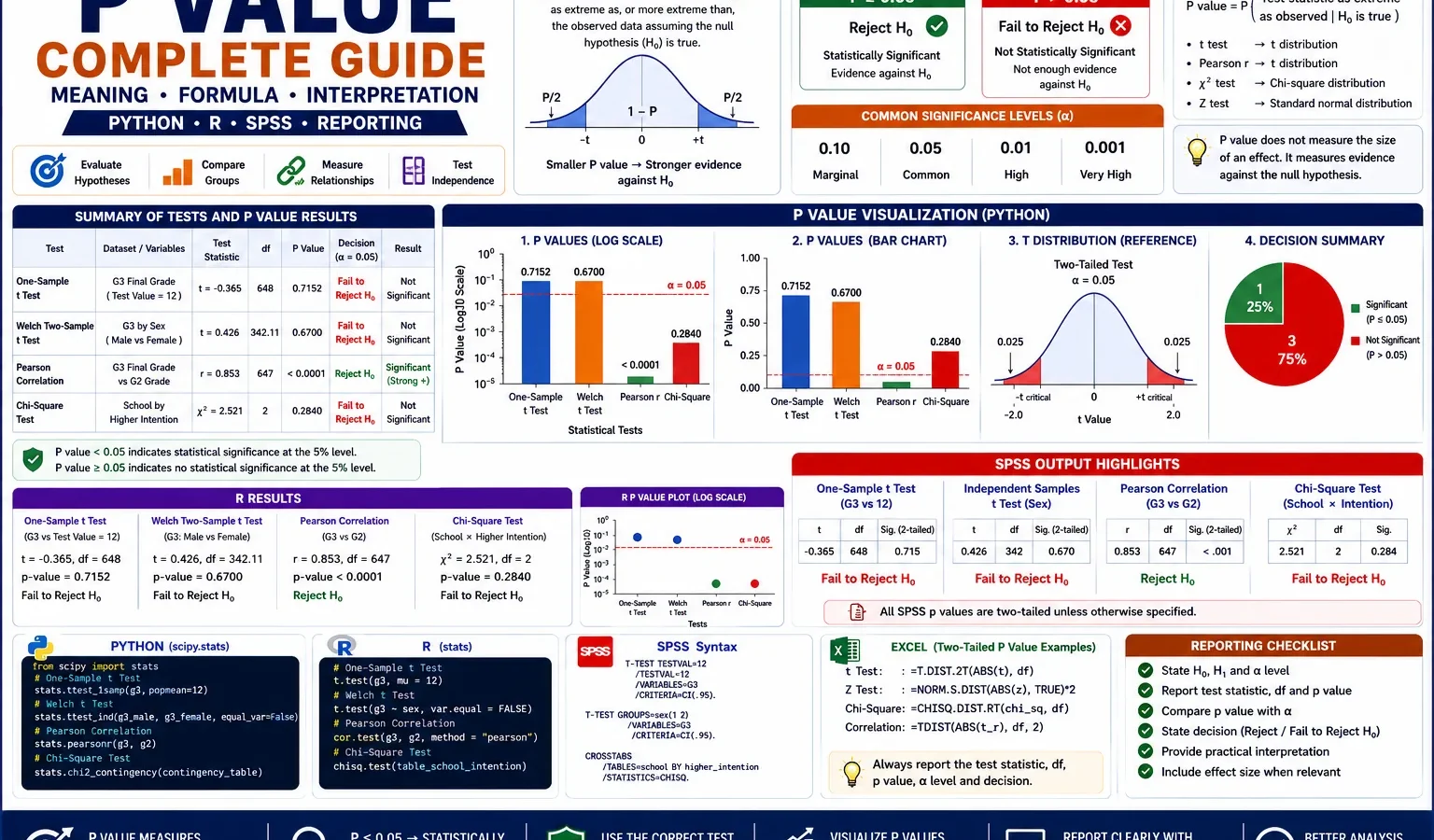
Hypothesis Testing, Alpha Level and Statistical Significance
P Value is the probability of getting a result at least as extreme as the observed result if the null hypothesis is true. This complete guide explains p value meaning, p value formula, how to find p value, how to calculate p value, and how to interpret p-values from a one-sample t test, Welch t test, Pearson correlation and chi-square test using Python, R and SPSS output.
Quick Answer: P Value Result
A P Value below the selected alpha level gives evidence against the null hypothesis. In this worked example, alpha was set at 0.05. The one-sample t test for G3 final grade produced t(648) = 15.030, p < .001. The independent samples t test comparing female and male G3 scores produced t(647) = 3.311, p = .001. The Pearson correlation between G2 and G3 produced r = .919, p < .001. The chi-square test for school and higher education intention produced χ²(1) = 12.024, p = .001.
Final report sentence: Across the selected examples, all reported p-values were below alpha = .05. Therefore, the null hypothesis was rejected for the one-sample t test, the independent samples t test, the Pearson correlation test and the chi-square test. The results support statistically significant evidence that G3 differs from the test value of 10, female and male G3 scores differ, G2 and G3 are strongly associated, and school is associated with higher education intention.
Important interpretation note: A small p-value does not prove that the null hypothesis is impossible. It means the observed result would be unlikely under the null hypothesis. It also does not measure the size or practical importance of an effect. For that, use confidence intervals, effect sizes and clear subject-matter interpretation.
Table of Contents
- What Is a P Value?
- P Value Formula and Decision Rule
- Dataset and Variables Used
- Null and Alternative Hypotheses
- Verified SPSS, Python and R Results
- Python Charts and Interpretation
- R Validation Charts
- How to Calculate P Value in Python, R, SPSS and Excel
- How to Report P Value Results
- Common Mistakes
- Download SPSS Output
- FAQs
What Is a P Value?
A P Value is a probability used in hypothesis testing. It tells us how unusual the observed result would be if the null hypothesis were true. A smaller p-value means the observed result is less compatible with the null hypothesis.
In most basic statistical work, the p-value is compared with an alpha level. The common alpha level is 0.05. If the p-value is below 0.05, the result is usually called statistically significant. If the p-value is equal to or above 0.05, there is not enough evidence to reject the null hypothesis.
The p-value is used in many common tests, including t tests, correlation tests, chi-square tests, ANOVA, regression, normality tests and assumption checks. The meaning stays the same: it measures evidence against the null hypothesis under a specific statistical model.
Plain meaning: A p-value answers this question: “If there were really no effect, no difference or no association, how surprising would this result be?” A very small p-value means the result is surprising under the null hypothesis.
For related guides, see One-Tailed T Test, One-Sample Z Test, One-Proportion Z Test, Confidence Interval and Effect Size.
P Value Formula and Decision Rule
There is no single p value formula for every test because each test uses its own reference distribution. A t test uses a t distribution. A chi-square test uses a chi-square distribution. A correlation test can use a t distribution after converting the correlation coefficient into a test statistic.
General p-value idea
P Value = Probability of observing a result as extreme as the test statistic,
assuming the null hypothesis is true.
Decision rule at alpha = 0.05
If p < 0.05: reject H0
If p >= 0.05: fail to reject H0
For a two-tailed t test, the p-value is based on how far the observed t statistic falls into either tail of the t distribution. For a chi-square test, the p-value is usually based on the right tail of the chi-square distribution. For Pearson correlation, the p-value tests whether the population correlation is zero.
SPSS reporting rule: SPSS may display very small p-values as .000. In final writing, do not report p = .000. Report it as p < .001.
Dataset and Variables Used
This p-value guide uses student performance data with 649 valid cases. The main numeric variables are G3 final grade and G2 second period grade. The group comparison uses sex group. The chi-square example uses school and higher education intention.
| Variable | N | Minimum | Maximum | Mean | Standard deviation | Use in this guide |
|---|---|---|---|---|---|---|
| G3 final grade | 649 | 0 | 19 | 11.91 | 3.231 | Used in the one-sample t test and group comparison. |
| G2 second period grade | 649 | 0 | 19 | 11.57 | 2.914 | Used as the predictor variable in the Pearson correlation example. |
G3 and G2 are strongly related grade variables. The correlation example uses them to show how a p-value tests whether an observed relationship is likely to be different from zero. The group comparison uses female and male G3 results. The chi-square example checks whether school and higher education intention are independent.
Before relying only on p-values, it is useful to review the shape and spread of the data. Related visual guides include Histogram Interpretation, Box Plot Interpretation, Q-Q Plot Normality Check and Descriptive Statistics.
Null and Alternative Hypotheses
Every p-value must be interpreted with a null hypothesis and an alternative hypothesis. Without hypotheses, the p-value has no clear meaning.
| Test | Null hypothesis H0 | Alternative hypothesis H1 | Decision rule |
|---|---|---|---|
| One-sample t test | The mean G3 final grade equals 10. | The mean G3 final grade is different from 10. | Reject H0 if p < .05. |
| Independent samples t test | Female and male students have the same mean G3 final grade. | Female and male students have different mean G3 final grades. | Reject H0 if p < .05. |
| Pearson correlation | The population correlation between G2 and G3 is zero. | The population correlation between G2 and G3 is not zero. | Reject H0 if p < .05. |
| Chi-square test | School and higher education intention are independent. | School and higher education intention are associated. | Reject H0 if p < .05. |
Alpha level used: The decision rule in this guide uses alpha = .05. When p is smaller than .05, the result gives enough evidence to reject H0 for that test.
Verified SPSS, Python and R Results
The SPSS output includes four p-value examples: a one-sample t test, an independent samples t test, a Pearson correlation and a chi-square test. Python and R charts then visualise the same logic using p-value bars, reference distributions, boxplots and scatterplots.
One-Sample T Test: G3 Compared with 10
The one-sample t test compared the G3 final grade mean with the test value of 10. The sample included 649 cases, with M = 11.91, SD = 3.231 and SE = 0.127. The test result was t(648) = 15.030, p < .001. The mean difference was 1.906, with a 95% confidence interval from 1.66 to 2.16.
Hypothesis decision: Since p < .001 is below alpha = .05, reject H0. The mean G3 final grade is statistically significantly different from 10. Because the mean difference is positive, the sample mean is higher than the test value.
Independent Samples T Test: G3 by Sex Group
The independent samples t test compared G3 final grade between female and male students. Female students had n = 383, M = 12.25 and SD = 3.124. Male students had n = 266, M = 11.41 and SD = 3.321. Levene’s test was not significant, F = 0.004, p = .950, so the equal variances assumed row can be used. The result was t(647) = 3.311, p = .001. The mean difference was 0.847, with a 95% confidence interval from 0.345 to 1.350.
Hypothesis decision: Since p = .001 is below alpha = .05, reject H0. The mean G3 final grade differs significantly between female and male students in this dataset. The female group has the higher mean score.
Welch T Test Result
The Welch version of the independent t test also supported the same conclusion: t(547.439) = 3.275, p = .001. The 95% confidence interval for the mean difference was 0.339 to 1.355. This confirms that the result remains statistically significant even when equal variance assumptions are relaxed.
Pearson Correlation: G2 and G3
The Pearson correlation tested whether G2 second period grade and G3 final grade were associated. The result was r = .919, p < .001, N = 649. This is a very strong positive correlation. Students with higher G2 scores tended to have higher G3 scores.
Hypothesis decision: Since p < .001 is below alpha = .05, reject H0. The population correlation between G2 and G3 is unlikely to be zero. The result supports a strong positive relationship between second period grade and final grade.
Chi-Square Test: School by Higher Education Intention
The chi-square test examined whether school and higher education intention were independent. For school GP, 32 students answered no and 391 answered yes. For school MS, 37 students answered no and 189 answered yes. Overall, 69 students answered no and 580 answered yes.
The Pearson chi-square result was χ²(1) = 12.024, p = .001. No expected cell count was below 5, and the minimum expected count was 24.03. Cramer’s V was .136, with p = .001.
Hypothesis decision: Since p = .001 is below alpha = .05, reject H0. School and higher education intention are statistically associated. The effect size, Cramer’s V = .136, suggests the association is small, even though it is statistically significant.
Summary of P Value Results
| Test | Statistic | df or N | P value | Decision at alpha = .05 | Plain interpretation |
|---|---|---|---|---|---|
| One-sample t test | t = 15.030 | df = 648 | p < .001 | Reject H0 | Mean G3 is significantly different from 10. |
| Independent samples t test | t = 3.311 | df = 647 | p = .001 | Reject H0 | Female and male G3 means differ significantly. |
| Welch t test | t = 3.275 | df = 547.439 | p = .001 | Reject H0 | The group difference remains significant with Welch correction. |
| Pearson correlation | r = .919 | N = 649 | p < .001 | Reject H0 | G2 and G3 have a very strong positive relationship. |
| Chi-square test | χ² = 12.024 | df = 1 | p = .001 | Reject H0 | School and higher education intention are associated. |
Python Charts and Interpretation
1. P Value Results Across Common Tests
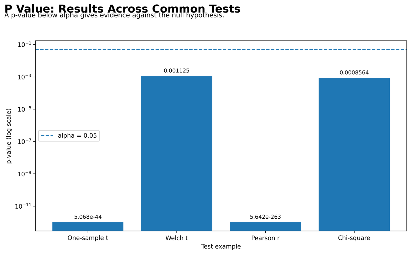
This chart places four test examples on the x-axis: one-sample t, Welch t, Pearson r and chi-square. The y-axis shows the p-value on a log scale, which is useful because the p-values are very small and would otherwise be hard to compare. The dashed horizontal line marks alpha = 0.05. Every bar is below the alpha line, so every test rejects the null hypothesis. The Pearson correlation has the smallest p-value, around 5.642e-263, showing extremely strong evidence against the null hypothesis of zero correlation. The Welch t and chi-square p-values are also below .05, but they are much larger than the Pearson result.
2. P Value Null Distribution Example
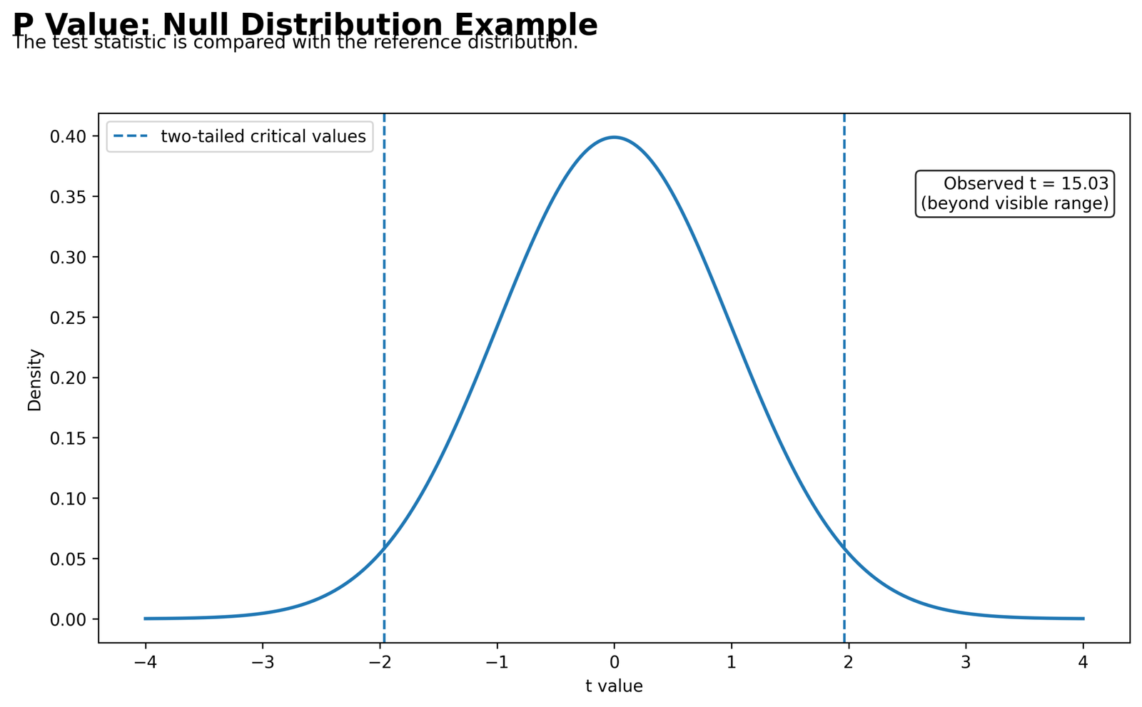
This chart shows the reference distribution used to judge a t statistic. The x-axis shows t values and the y-axis shows density. The dashed vertical lines mark the approximate two-tailed critical values near -1.96 and 1.96. The observed one-sample t statistic is 15.03, which is beyond the visible range of the plot. That is why the p-value is extremely small. In hypothesis terms, the observed statistic is far away from what H0 would usually produce, so H0 is rejected.
3. P Value Practical Scale
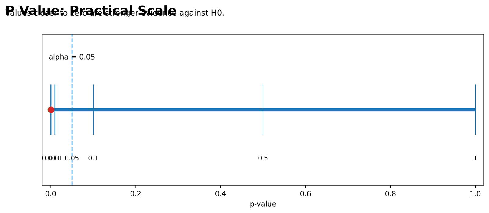
This chart turns the p-value decision into a practical scale from 0 to 1. The dashed line marks alpha = 0.05. Values to the left of that line are statistically significant at the .05 level. The red point near zero represents a very small p-value. The chart makes the main decision rule easy to see: when p is smaller than alpha, reject the null hypothesis. It also shows why a p-value should not be read as a percent chance that H0 is true. It is a probability of the data pattern under H0, not the probability that H0 itself is true.
4. P Value Example: Correlation
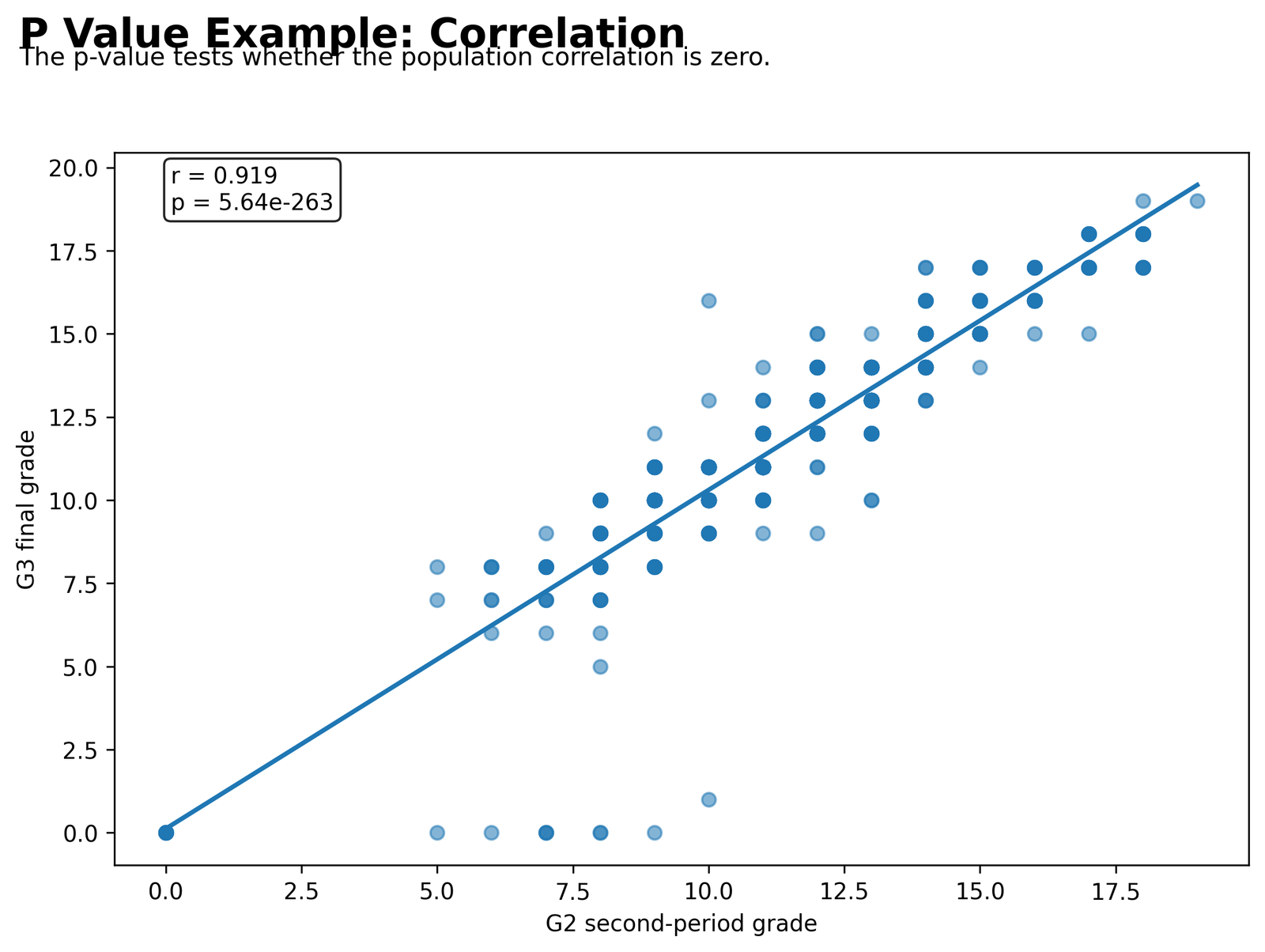
This scatterplot shows G2 second period grade on the x-axis and G3 final grade on the y-axis. The fitted line slopes upward, meaning higher G2 values are linked with higher G3 values. The chart annotation reports r = .919 and p = 5.64e-263. This means the observed relationship is very strong and the p-value gives overwhelming evidence against the null hypothesis that the population correlation is zero. The chart also reminds us that statistical significance and strength are different ideas. The p-value tells us the evidence against H0, while r tells us the strength and direction of the relationship.
R Validation Charts
The R validation charts confirm the same p-value logic using distribution checks, group comparison, p-value summaries and Pearson versus Spearman correlation. These charts support the same statistical decisions from the SPSS and Python outputs.
1. Parametric vs Nonparametric Distribution Check
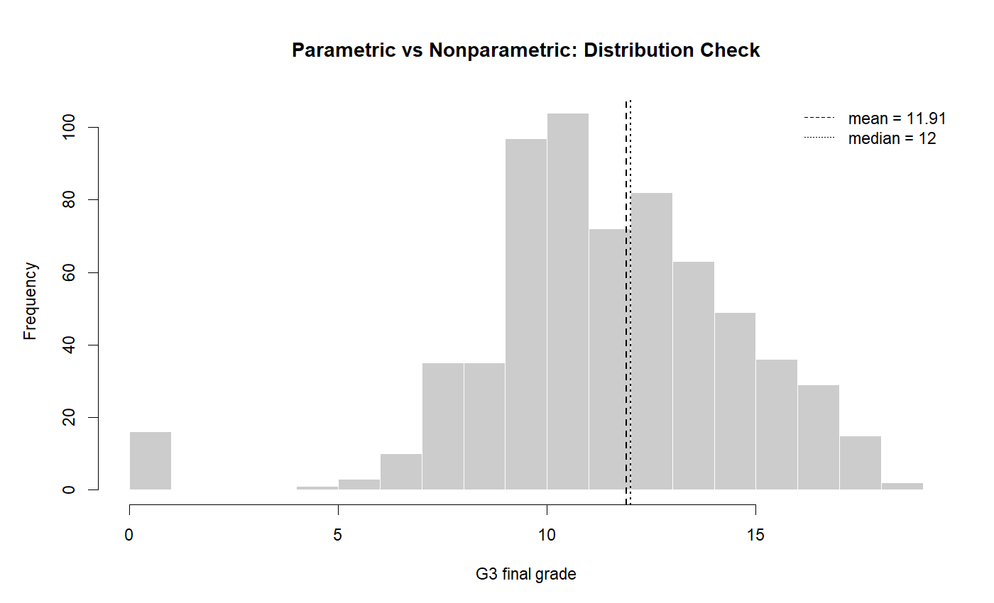
This chart checks the distribution of G3 final grade before interpreting parametric tests. The x-axis shows G3 values and the y-axis shows frequency. The mean is about 11.91 and the median is 12, so the centre is fairly close. Most scores are grouped around the middle range, but there are low values near zero. The chart is useful because p-values from t tests are usually interpreted together with distribution shape, sample size and robustness. With N = 649, the t test is generally stable, but the visual check still helps explain the data context.
2. R P Value Summary
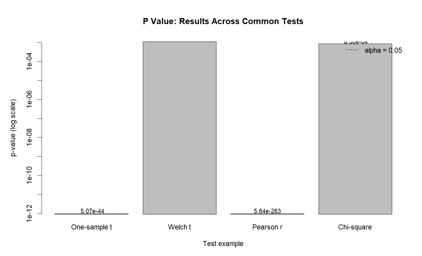
The R p-value summary repeats the same core message as the Python chart. The p-values are plotted on a log scale, so extremely small values can be shown beside less extreme but still significant values. The one-sample t and Pearson correlation p-values are extremely small. The Welch t and chi-square p-values are also below alpha = .05. This chart confirms that the null hypothesis is rejected across all four examples.
3. G3 by Sex Boxplot
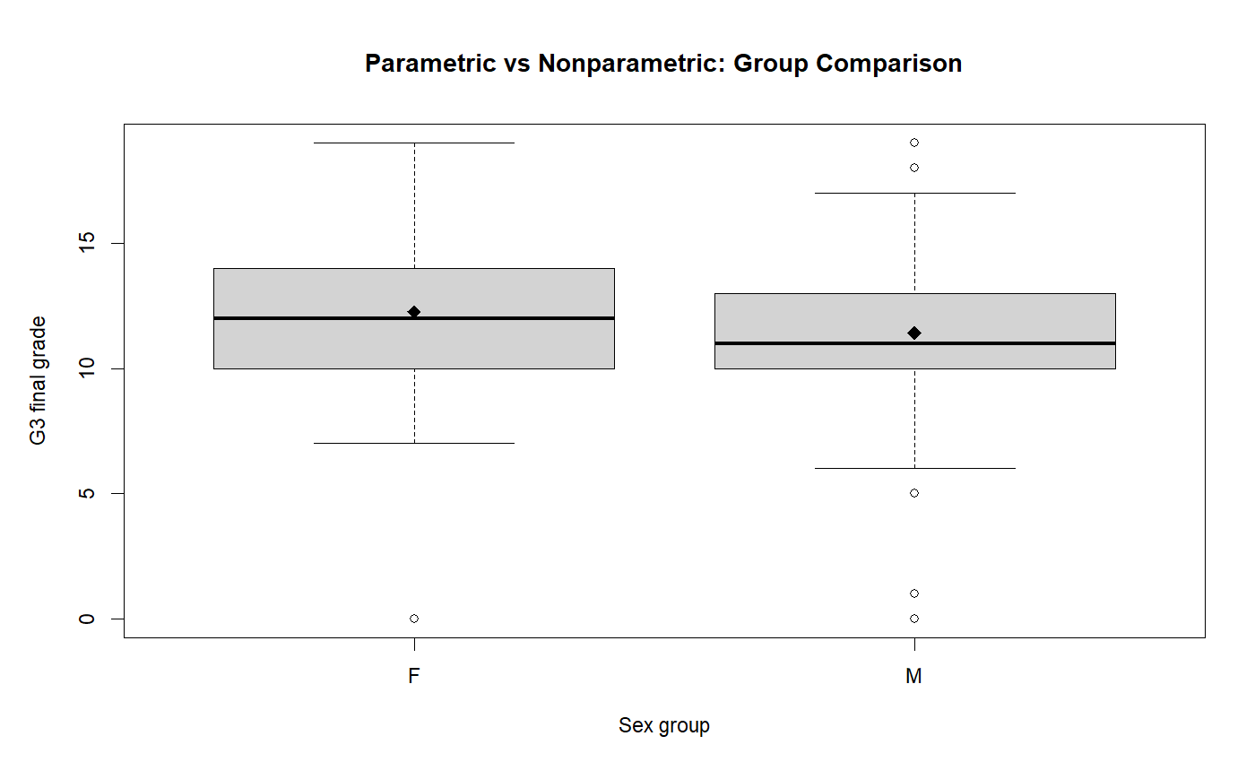
This boxplot shows the group comparison behind the independent t test. The x-axis shows the sex group and the y-axis shows G3 final grade. The female group has a slightly higher centre than the male group, which matches the SPSS group means: 12.25 for female students and 11.41 for male students. The boxes also show overlap, so the difference is not a complete separation between groups. The p-value of .001 says the mean difference is statistically significant, while the boxplot shows the practical shape and overlap of the two groups.
4. R T Distribution Reference
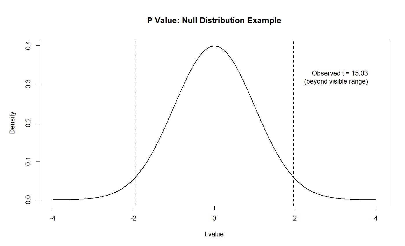
This R chart shows the same null distribution idea. Under H0, most t statistics would fall near the centre of the distribution. The critical values mark the tail boundaries. The observed t statistic of 15.03 is far outside the visible area, meaning it falls deep in the tail. That is why the one-sample t test p-value is far below .001.
5. Parametric vs Nonparametric P-Value Comparison
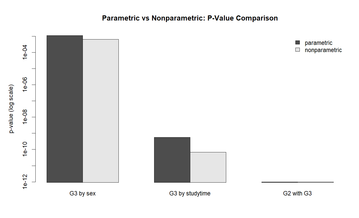
This chart compares parametric and nonparametric p-values for selected examples, including G3 by sex, G3 by studytime and G2 with G3. The y-axis uses a log scale because the p-values are small. The bars show that both parametric and nonparametric approaches can lead to the same general conclusion when the evidence is strong. This does not mean the methods are identical. It means that, in these examples, the results are consistently below alpha = .05.
6. R P Value Practical Scale
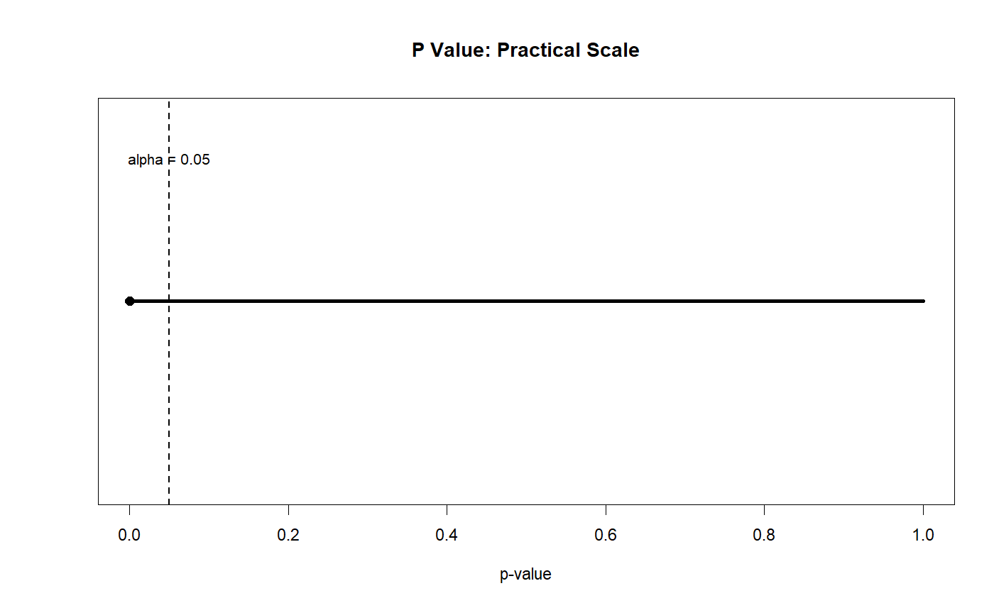
This practical scale shows the decision threshold clearly. The dashed line marks alpha = .05. The example p-value appears far to the left of that threshold, so the result is statistically significant. This chart is helpful for beginners because it shows that “small enough” depends on the alpha level chosen before interpretation.
7. R Correlation P Value
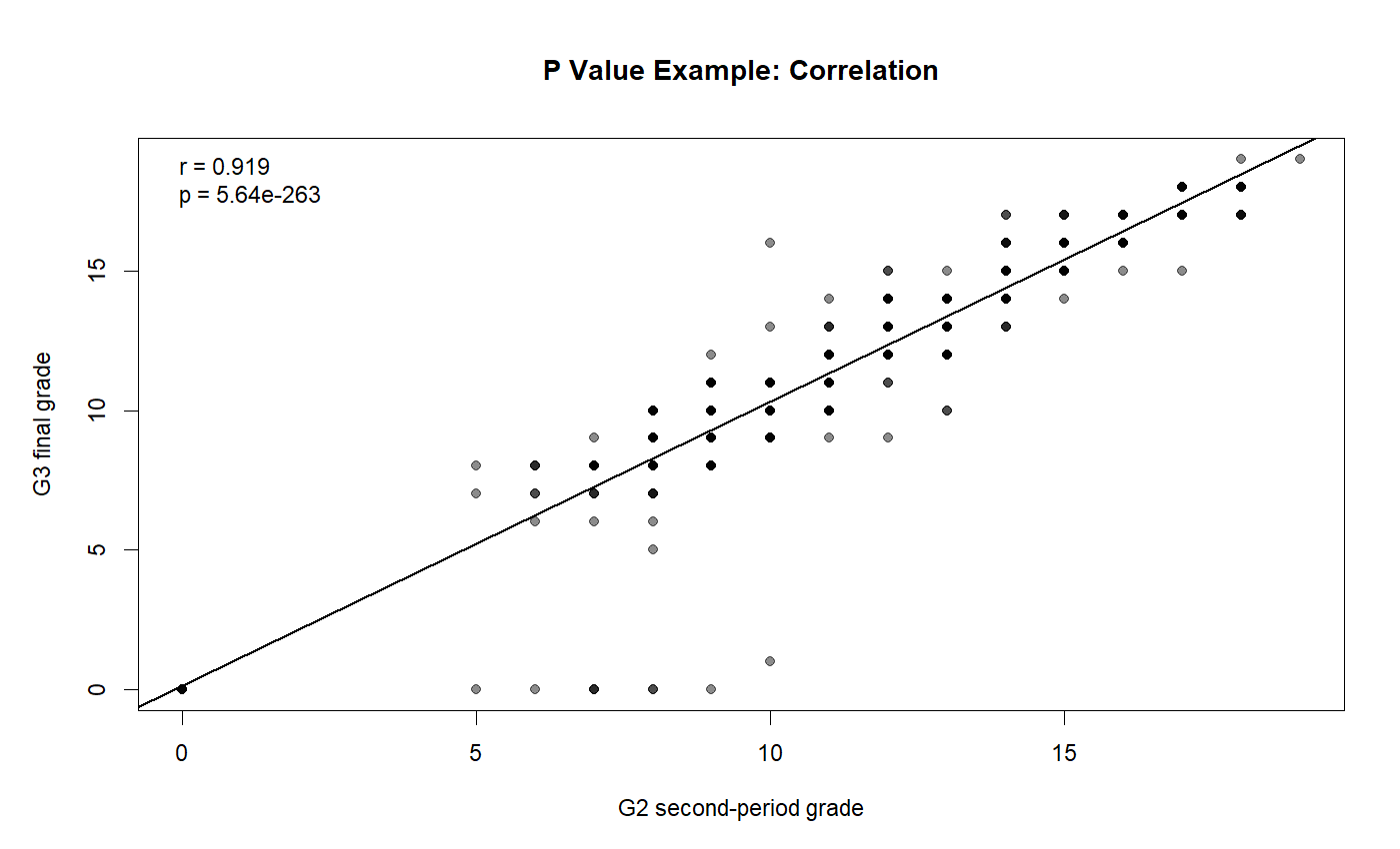
The R scatterplot again shows a strong upward pattern between G2 and G3. The annotation reports r = .919 and p = 5.64e-263. The fitted line confirms the positive relationship. The p-value tests whether this relationship could reasonably be zero in the population. Since the p-value is far below .05, H0 is rejected.
8. Pearson vs Spearman Correlation Choice
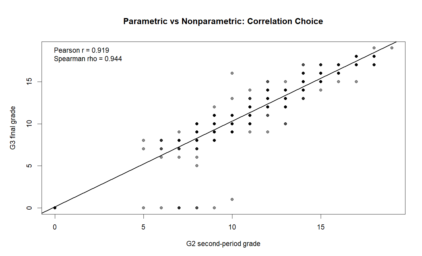
This chart compares two correlation choices. Pearson correlation is shown as r = .919, while Spearman rho is shown as .944. Both values indicate a very strong positive association. Pearson focuses on linear association, while Spearman focuses on rank-based association. Since both are high, the conclusion is stable: G2 and G3 are strongly related.
How to Calculate P Value in Python, R, SPSS and Excel
Calculate P Value in Python
Python can calculate p-values for t tests, correlations and chi-square tests using SciPy.
import pandas as pd
from scipy import stats

# One-sample t test: H0 mean G3 = 10
t_stat, p_value = stats.ttest_1samp(df["G3"].dropna(), popmean=10)
print(t_stat, p_value)

# Independent samples t test by sex group
female = df.loc[df["sex"] == "F", "G3"].dropna()
male = df.loc[df["sex"] == "M", "G3"].dropna()

t_equal, p_equal = stats.ttest_ind(female, male, equal_var=True)
t_welch, p_welch = stats.ttest_ind(female, male, equal_var=False)

print("Equal variance t:", t_equal, p_equal)
print("Welch t:", t_welch, p_welch)

# Pearson correlation
r, p_corr = stats.pearsonr(df["G2"], df["G3"])
print("Pearson r:", r, "p:", p_corr)

# Chi-square test
table = pd.crosstab(df["school"], df["higher"])
chi2, p_chi, dof, expected = stats.chi2_contingency(table)
print("Chi-square:", chi2, "p:", p_chi, "df:", dof)
Calculate P Value in R
R can calculate the same p-values using built-in statistical functions.
# One-sample t test
t.test(student$G3, mu = 10)

# Independent samples t test
t.test(G3 ~ sex, data = student, var.equal = TRUE)

# Welch t test
t.test(G3 ~ sex, data = student, var.equal = FALSE)

# Pearson correlation
cor.test(student$G2, student$G3, method = "pearson")

# Spearman correlation
cor.test(student$G2, student$G3, method = "spearman")

# Chi-square test
tab <- table(student$school, student$higher)
chisq.test(tab)
Calculate P Value in SPSS
SPSS reports p-values in the Sig. column. For very small p-values displayed as .000, report p < .001.
* One-sample t test.
T-TEST
 /TESTVAL=10
 /MISSING=ANALYSIS
 /VARIABLES=G3
 /CRITERIA=CI(.95).

* Independent samples t test.
T-TEST GROUPS=sex('F' 'M')
 /MISSING=ANALYSIS
 /VARIABLES=G3
 /CRITERIA=CI(.95).

* Pearson correlation.
CORRELATIONS
 /VARIABLES=G2 G3
 /PRINT=TWOTAIL NOSIG
 /MISSING=PAIRWISE.

* Chi-square test.
CROSSTABS
 /TABLES=school BY higher
 /STATISTICS=CHISQ PHI
 /CELLS=COUNT EXPECTED ROW COLUMN.
Calculate P Value in Excel
Excel can calculate p-values for common tests with built-in formulas. It is useful for quick checks, but Python, R and SPSS give more complete statistical output.
| Excel task | Example formula | Purpose |
|---|---|---|
| Two-tailed p-value from t statistic | =T.DIST.2T(ABS(t_stat), df) | Calculates a two-tailed t test p-value. |
| Right-tailed p-value from chi-square | =CHISQ.DIST.RT(chi_square, df) | Calculates a chi-square p-value. |
| Two-sample t test p-value | =T.TEST(range1, range2, 2, 2) | Calculates a two-tailed two-sample equal variance t test. |
| Welch t test p-value | =T.TEST(range1, range2, 2, 3) | Calculates a two-tailed unequal variance t test. |
| Correlation coefficient | =CORREL(range_x, range_y) | Calculates Pearson correlation. Additional steps are needed for the p-value. |
How to Report P Value Results
A strong p-value report should include the test name, statistic, degrees of freedom where available, p-value, confidence interval when available, and a plain explanation of the hypothesis decision.
One-sample t test report: A one-sample t test showed that the mean G3 final grade was significantly different from 10, t(648) = 15.030, p < .001. The mean difference was 1.906, 95% CI [1.66, 2.16]. Therefore, the null hypothesis that the mean G3 score equals 10 was rejected.
Independent t test report: Female students had a higher mean G3 final grade than male students. The equal variances assumed test was significant, t(647) = 3.311, p = .001, with a mean difference of 0.847, 95% CI [0.345, 1.350]. Therefore, the null hypothesis of equal group means was rejected.
Correlation report: G2 second period grade and G3 final grade were strongly positively correlated, r = .919, p < .001, N = 649. Therefore, the null hypothesis that the population correlation equals zero was rejected.
Chi-square report: A chi-square test showed a significant association between school and higher education intention, χ²(1, N = 649) = 12.024, p = .001. Cramer's V was .136, suggesting a small association.
Common Mistakes
1. Saying p-value is the probability that H0 is true
This is incorrect. A p-value is calculated under the assumption that H0 is true. It does not give the probability that H0 itself is true.
2. Reporting p = .000
SPSS may display very small p-values as .000. In final writing, report them as p < .001.
3. Treating statistical significance as practical importance
A small p-value does not always mean the effect is large or useful. Always review effect size, confidence interval, sample size and real-world meaning.
4. Ignoring the null and alternative hypotheses
The p-value only makes sense when the null and alternative hypotheses are clear. Always state what H0 and H1 mean for the test.
5. Using p-value alone to choose between parametric and nonparametric tests
Method choice should consider data type, distribution, sample size, outliers, assumptions and the research question. The p-value is only one part of the analysis.
Download SPSS Output and Verification Files
The SPSS output PDF verifies the descriptive statistics, one-sample t test, independent t test, Pearson correlation and chi-square p-value results used in this guide.
External References for P Value
This post uses verified Python, R and SPSS outputs together with standard statistical testing references and software documentation.
FAQs About P Value
What is a p value?
A p value is the probability of observing a result at least as extreme as the one found in the sample, assuming the null hypothesis is true.
What does p value mean in statistics?
In statistics, a p value measures how compatible the observed result is with the null hypothesis. A smaller p value gives stronger evidence against the null hypothesis.
What is the common p value cutoff?
The common cutoff is alpha = .05. If p < .05, the result is often considered statistically significant.
How do you interpret p < .001?
p < .001 means the result is very unlikely under the null hypothesis. It gives strong evidence against H0, but it still does not prove that H0 is impossible.
What was the p value for the one-sample t test?
The one-sample t test for G3 final grade produced t(648) = 15.030 with p < .001. The null hypothesis that the mean G3 score equals 10 was rejected.
What was the p value for the G3 by sex t test?
The independent samples t test produced p = .001. This means the mean G3 scores differed significantly between female and male students.
What was the p value for the Pearson correlation?
The Pearson correlation between G2 and G3 produced r = .919 with p < .001. This shows a very strong positive relationship.
What was the p value for the chi-square test?
The chi-square test for school by higher education intention produced χ²(1) = 12.024 with p = .001. This supports an association between school and higher intention.
Can a small p value prove a result is important?
No. A small p value shows statistical evidence against H0, but practical importance should be judged using effect size, confidence interval, sample size and context.
Why should p = .000 not be reported?
Because the p value is not exactly zero. SPSS displays .000 when the value is very small. The correct report is p < .001.

