
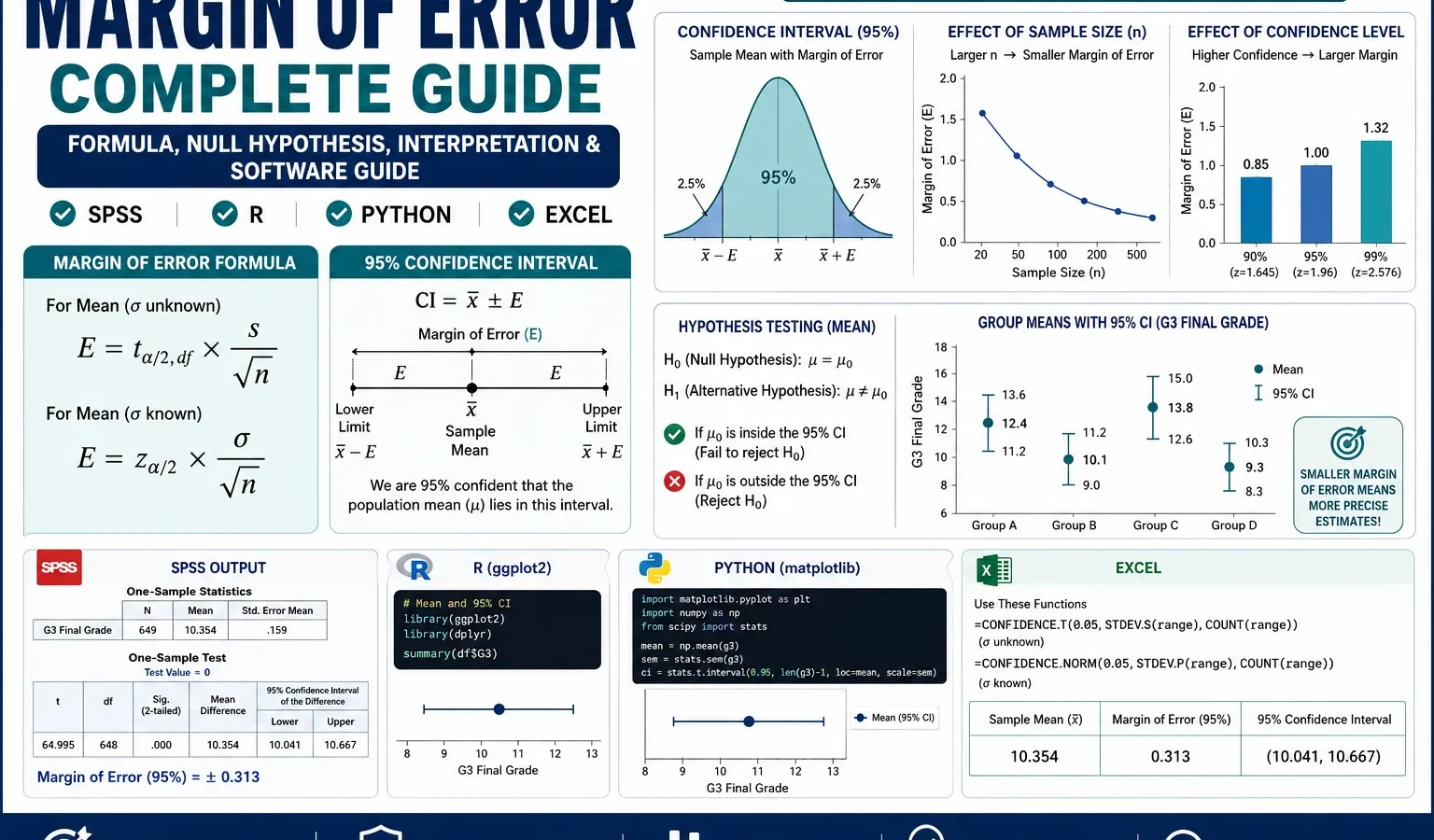
Confidence Interval Width, Standard Error and Hypothesis Decision
Margin of error tells how far a sample estimate may reasonably be from the true population value at a chosen confidence level. In this guide, margin of error is explained with formula, null hypothesis, alternative hypothesis, confidence interval interpretation, SPSS output, R charts, Python charts and Excel method using G3 final grade from the student-por.csv dataset.
Quick Answer: Margin of Error Result for G3
The main outcome was G3 final grade. The SPSS and Python/R outputs show N = 649, mean = 11.9060, standard deviation = 3.2307, standard error = 0.1268, t critical value = 1.9636 and 95% margin of error = 0.2490. Therefore, the 95% confidence interval for the mean G3 score is approximately 11.6570 to 12.1550.
Hypothesis decision example: Margin of error is mainly an estimation statistic, but it can support a hypothesis decision when a comparison value is stated. If the comparison value is μ0 = 12, the null hypothesis is H0: μ = 12 and the alternative hypothesis is H1: μ ≠ 12. Because 12 falls inside the 95% confidence interval [11.6570, 12.1550], we fail to reject the null hypothesis at the 5% level. The sample mean is slightly below 12, but the confidence interval says that 12 is still a plausible population mean.
Final report sentence: The margin of error analysis for G3 final grade showed M = 11.9060, SE = 0.1268 and a 95% t-based margin of error of 0.2490. The 95% confidence interval was [11.6570, 12.1550]. Using 12 as a comparison value, the interval contains 12, so the null hypothesis that the population mean equals 12 is not rejected. The result suggests that the sample mean is estimated precisely, but it is not statistically different from 12 using the confidence-interval decision rule.
Important interpretation note: Margin of error is not the same as standard error. Standard error is the estimated standard deviation of the sample mean. Margin of error multiplies the standard error by a critical value, such as a z critical value or t critical value. For this G3 analysis, the standard error is about 0.1268, while the 95% margin of error is about 0.2490.
Table of Contents
- What Is Margin of Error?
- Margin of Error Formula
- Null and Alternative Hypothesis for Margin of Error
- Dataset and Clean SPSS-Ready Files Used
- Verified SPSS, R and Python Results
- Python Charts and Interpretation
- R Validation Charts
- How to Calculate Margin of Error in Python, R, SPSS and Excel
- How to Report Margin of Error
- Common Mistakes
- Download SPSS Output
- FAQs
What Is Margin of Error?
Margin of error is the distance added to and subtracted from a sample estimate to create a confidence interval. If the sample mean is 11.906 and the 95% margin of error is 0.249, the 95% confidence interval is calculated as 11.906 ± 0.249, giving approximately 11.657 to 12.155.
In practical research writing, margin of error answers this question: How precise is the estimate? A smaller margin of error means the sample mean is estimated more precisely. A larger margin of error means there is more uncertainty around the estimate. In this student performance example, the 95% margin of error for G3 is only about one-quarter of a grade point, so the estimate of the mean final grade is fairly precise.
Margin of error is closely connected with confidence intervals, the Central Limit Theorem, descriptive statistics and hypothesis testing. When a confidence interval is used to judge a comparison value, it can support decisions similar to a one-sample z test or a t test. For distribution checks before interpretation, also see histogram interpretation, Q-Q plot normality check and box plot interpretation.
Practical meaning: The sample mean tells the best estimate from the observed data. The margin of error tells how much uncertainty surrounds that estimate. In this analysis, the G3 mean is 11.9060, and the 95% margin of error is 0.2490, so the likely population mean range is narrow.
Margin of Error Formula
The general margin of error formula is:
Margin of Error = Critical Value × Standard ErrorFor a mean, the standard error is:
Standard Error = s / √nWhere s is the sample standard deviation and n is the sample size. When the population standard deviation is unknown, a t critical value is usually preferred:
MOE = t critical × (s / √n)| Formula part | G3 value | Explanation |
|---|---|---|
| Sample size | 649 | Number of valid G3 observations. |
| Sample mean | 11.9060 | Best estimate of the population mean G3 final grade. |
| Standard deviation | 3.2307 | Spread of individual G3 scores. |
| Standard error | 0.1268 | Estimated uncertainty of the sample mean. |
| 95% z critical value | 1.9600 | Normal critical value for a 95% interval. |
| 95% t critical value | 1.9636 | t critical value used when the population standard deviation is unknown. |
| 95% t-based margin of error | 0.2490 | Final margin of error used for the confidence interval. |
Formula using the G3 result: The t-based 95% margin of error is 1.9636 × 0.1268 = 0.2490. Therefore, the 95% confidence interval is 11.9060 − 0.2490 = 11.6570 and 11.9060 + 0.2490 = 12.1550.
Null and Alternative Hypothesis for Margin of Error
Margin of error itself is an estimation tool, not a standalone hypothesis test. However, confidence intervals created from the margin of error can be used to support a hypothesis decision when a comparison value is provided. In this post, the comparison value is 12, because 12 is close to the observed mean and is also a natural grade reference point.
| Hypothesis | Statement | Meaning for G3 final grade |
|---|---|---|
| Null hypothesis | H0: μ = 12 | The population mean G3 final grade is equal to 12. |
| Alternative hypothesis | H1: μ ≠ 12 | The population mean G3 final grade is different from 12. |
| Confidence interval rule | Check whether 12 lies inside the 95% CI. | If 12 is inside the interval, fail to reject H0; if 12 is outside, reject H0. |
The observed 95% confidence interval for G3 is [11.6570, 12.1550]. Since 12 is inside this interval, the result does not provide enough evidence to reject the null hypothesis at the 5% level.
Hypothesis decision: Fail to reject the null hypothesis. The population mean G3 final grade may plausibly be 12 because 12 lies inside the 95% confidence interval. The sample mean is 11.9060, but the margin of error shows that this difference from 12 is small enough to be explained by sampling uncertainty.
Reporting caution: The hypothesis decision depends on the comparison value. If a different target value is chosen, the decision can change. Always state the null hypothesis, alternative hypothesis, confidence level and interval before making a conclusion.
Dataset and Clean SPSS-Ready Files Used
This margin of error example uses the student-por.csv student performance dataset. The main outcome variable is G3 final grade. The uploaded SPSS output confirms that the cleaned file contained 33 variables and 649 cases. The same G3 outcome was used in Python, R and SPSS so the charts and tables are directly comparable.
SPSS workflow rule: A clean SPSS-ready data file was created before running the SPSS output. This prevents CSV import errors and keeps variables such as school, sex, age, absences, G1, G2 and G3 correctly defined.
| Item | Value or file | Explanation |
|---|---|---|
| Main dataset | student-por.csv | Student performance dataset used for the worked example. |
| SPSS-ready file | spss_ready_data.csv | Clean file written for SPSS output generation. |
| Main variable | G3 final grade | Main outcome used for margin of error and confidence interval calculation. |
| Valid N | 649 | All G3 cases were valid in the SPSS output. |
| Hypothesis comparison value | μ0 = 12 | Used to demonstrate confidence-interval-based hypothesis decision. |
| Software workflow | Python, R, SPSS and Excel | Python and R produced charts; SPSS produced verification output; Excel formulas are shown for manual calculation. |
External dataset source: UCI Machine Learning Repository: Student Performance dataset.
Verified SPSS, R and Python Results
The SPSS output gives the official descriptive statistics and confidence interval values. Python and R reproduce the margin of error visually through error bars, confidence-level comparisons, school-group intervals, sample-size curves and numeric-variable comparisons. The results agree: the G3 mean is estimated precisely, with a 95% margin of error of about 0.249.
Main G3 Margin of Error Result
| Statistic | Value | Interpretation |
|---|---|---|
| Valid N | 649 | The confidence interval is based on 649 valid G3 scores. |
| Mean | 11.9060 | The sample estimate of the population mean final grade. |
| Standard deviation | 3.2307 | The spread of individual G3 scores. |
| Standard error | 0.1268 | The estimated sampling uncertainty of the mean. |
| z critical value | 1.9600 | Normal critical value for 95% confidence. |
| t critical value | 1.9636 | t critical value used for the t-based interval. |
| 95% z-based MOE | 0.2486 | Very close to the t-based result because N is large. |
| 95% t-based MOE | 0.2490 | Main reported margin of error. |
| 95% confidence interval | 11.6570 to 12.1550 | The likely range for the population mean G3 final grade. |
Hypothesis Result Using the 95% Confidence Interval
| Component | Result | Decision |
|---|---|---|
| Null hypothesis | H0: μ = 12 | Assumes the population mean G3 final grade equals 12. |
| Alternative hypothesis | H1: μ ≠ 12 | Assumes the population mean G3 final grade differs from 12. |
| Observed mean | 11.9060 | The sample mean is slightly below 12. |
| 95% CI | 11.6570 to 12.1550 | The interval includes 12. |
| Decision | Fail to reject H0 | There is not enough evidence to say that the population mean differs from 12. |
SPSS Descriptive and Normality Output
| SPSS result | Value | Meaning for margin of error |
|---|---|---|
| Mean | 11.91 | Rounded SPSS mean for G3 final grade. |
| Standard error | 0.127 | Rounded SPSS standard error used to understand estimate precision. |
| 95% confidence interval | 11.66 to 12.16 | Rounded SPSS interval matching the detailed calculation. |
| Median | 12.00 | Central grade is close to the sample mean. |
| Standard deviation | 3.231 | Individual grades vary by about 3.23 points. |
| Interquartile range | 4 | The middle 50% of grades cover about four grade points. |
| Skewness | -0.913 | The distribution has a low-score tail, so charts should be checked. |
| Kurtosis | 2.712 | The distribution is more heavy-tailed than a normal distribution. |
| Kolmogorov-Smirnov | D = .124, p < .001 | Normality is rejected; margin of error is still useful because N is large. |
| Shapiro-Wilk | W = .926, p < .001 | Confirms that G3 is not perfectly normal. |
Group Results by School and Sex
| Grouping variable | Group | N | Mean | SD | SE | Interpretation |
|---|---|---|---|---|---|---|
| School | GP | 423 | 12.58 | 2.626 | 0.128 | Higher mean and narrower interval because the group is larger and less variable. |
| School | MS | 226 | 10.65 | 3.834 | 0.255 | Lower mean and wider interval because this group has more variability and fewer cases. |
| Sex | F | 383 | 12.25 | 3.124 | 0.160 | Female students have a higher mean than male students in this sample. |
| Sex | M | 266 | 11.41 | 3.321 | 0.204 | Male students have a lower mean and wider standard error than female students. |
Python Charts and Interpretation
1. Margin of Error for the Main Outcome
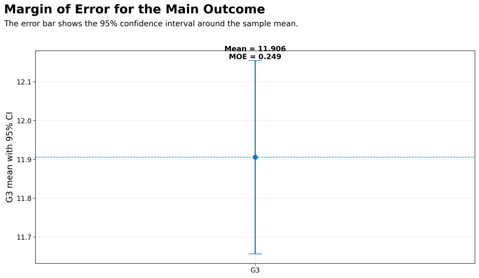
This chart shows the main margin of error result for G3 final grade. The central point is the sample mean, 11.906. The vertical error bar shows the 95% confidence interval around that mean. The chart annotation reports MOE = 0.249, so the interval extends about 0.249 points below and above the mean. This creates an interval of approximately 11.657 to 12.155. The dashed horizontal line marks the mean level, helping the reader see that the interval is centered on the sample estimate. The caps at the top and bottom of the vertical line show the confidence interval limits. Practically, the chart says that the estimated average G3 score is precise because the interval is narrow relative to the full grade scale from 0 to 19. For the hypothesis section, this chart is also important because the comparison value 12 lies inside the confidence interval. Therefore, using a two-sided 95% confidence interval decision rule, we fail to reject the null hypothesis that the population mean equals 12.
2. Margin of Error Increases with Confidence Level
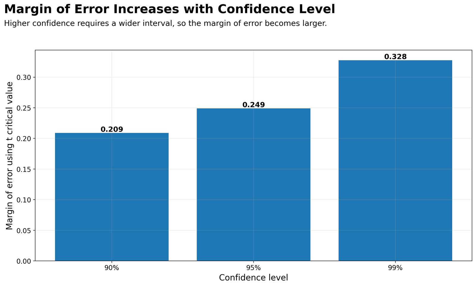
This chart explains why confidence level changes the width of a confidence interval. The 90% margin of error is 0.209, the 95% margin of error is 0.249, and the 99% margin of error is 0.328. The bars become taller as the confidence level increases because a higher confidence level requires a larger critical value. In simple words, if we want to be more confident that the interval captures the population mean, we must accept a wider interval. This is the trade-off between confidence and precision. A 90% interval is narrower but less confident. A 99% interval is wider but more confident. The 95% level is commonly used because it balances precision and confidence. For reporting, the post uses the 95% margin of error because it is the standard choice in many statistical reports. For hypothesis interpretation, using a 99% interval would make it even harder to reject the null hypothesis because the interval would be wider.
3. Margin of Error by School
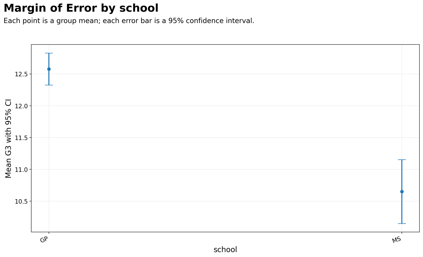
This chart compares G3 mean scores by school. Each point is a group mean, and each vertical error bar is a 95% confidence interval around that group mean. The GP group has N = 423, mean = 12.58, SD = 2.626 and SE = 0.128. The MS group has N = 226, mean = 10.65, SD = 3.834 and SE = 0.255. The GP interval is narrower because the group has more cases and less variation. The MS interval is wider because the group has fewer cases and more spread in scores. Visually, the GP and MS intervals are separated, suggesting that GP students have a higher average G3 score than MS students in this dataset. However, this chart is still an estimation chart, not a complete group-difference test by itself. For a formal group comparison, the next step would be a t test or regression model, and assumptions such as variance equality can be checked with Levene test or Brown-Forsythe test. The chart supports the practical conclusion that school-level mean estimates differ and that MS has a less precise estimate because its error bar is wider.
4. Sample Size and Margin of Error

This line chart shows the relationship between sample size and margin of error. The curve drops sharply at small sample sizes and then gradually flattens as sample size becomes larger. This happens because standard error is calculated as s / √n. Increasing sample size reduces standard error, but the reduction follows the square-root rule, not a straight-line rule. That means the first increases in sample size produce large gains in precision, while later increases produce smaller gains. For example, a very small sample has a wide margin of error because the estimate is unstable. As sample size moves toward the full dataset size of 649, the margin of error approaches about 0.249. This chart is useful for planning research because it shows why larger samples create narrower confidence intervals. It also supports the Central Limit Theorem idea that larger samples produce more stable estimates. For a deeper explanation of why sample means stabilize as sample size increases, see the Central Limit Theorem guide.
5. Largest 95% Margins of Error Across Numeric Variables
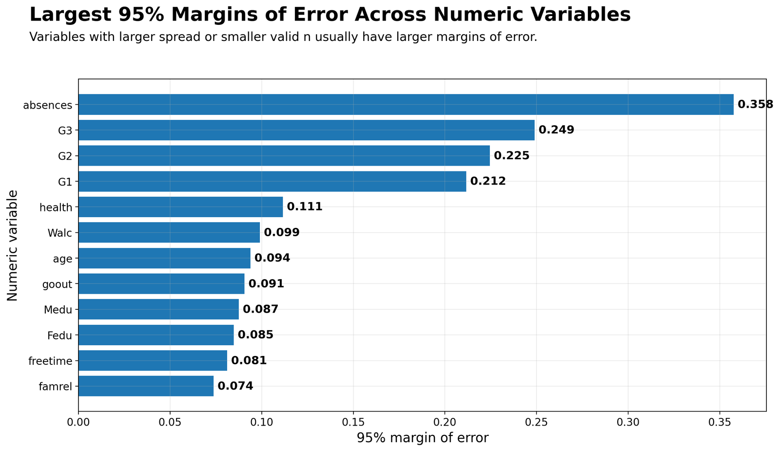
This horizontal bar chart compares 95% margin of error values across numeric variables. The largest margin of error appears for absences = 0.358, followed by G3 = 0.249, G2 = 0.225, G1 = 0.212, health = 0.111, Walc = 0.099, age = 0.094, goout = 0.091, Medu = 0.087, Fedu = 0.085, freetime = 0.081 and famrel = 0.074. The reason absences has the largest margin of error is that it has a much larger spread than most other variables. Even if the valid sample size is the same, a variable with a larger standard deviation will usually have a larger standard error and therefore a larger margin of error. The grade variables G3, G2 and G1 also have larger margins of error than ordinal variables such as famrel or freetime because grades vary across a wider numeric scale. This chart helps readers understand that margin of error is not only about sample size. It is also about variability. A large sample can still have a wider interval if the variable itself is highly spread out.
R Validation Charts
The R charts reproduce the same margin of error findings using a separate software workflow. This confirms that the result is not limited to Python or SPSS. The R outputs support the same main conclusion: G3 has a mean of about 11.906, a 95% margin of error of about 0.249, and a 95% confidence interval that includes 12.
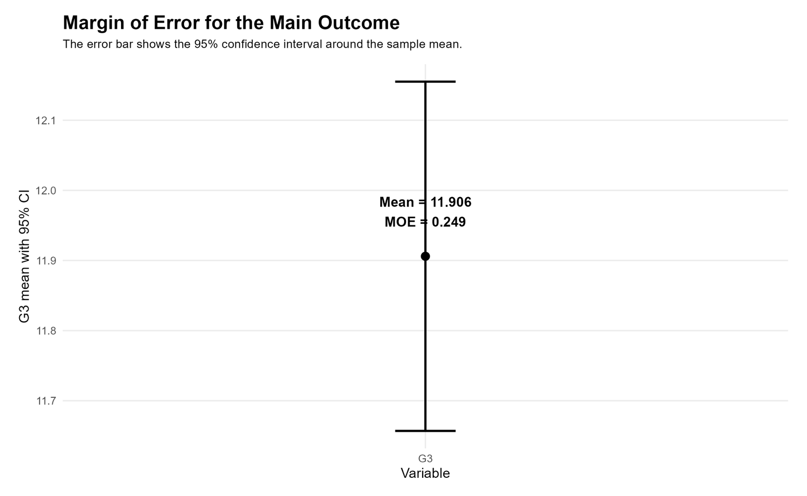
The R main-outcome chart validates the same confidence interval shown in Python. The point marks the G3 sample mean, and the vertical interval shows the 95% confidence interval. The annotation reports mean = 11.906 and MOE = 0.249. This confirms that the confidence interval is narrow and that the mean estimate is fairly precise. Since the interval still covers the comparison value 12, the hypothesis decision remains the same: fail to reject the null hypothesis that the population mean equals 12.
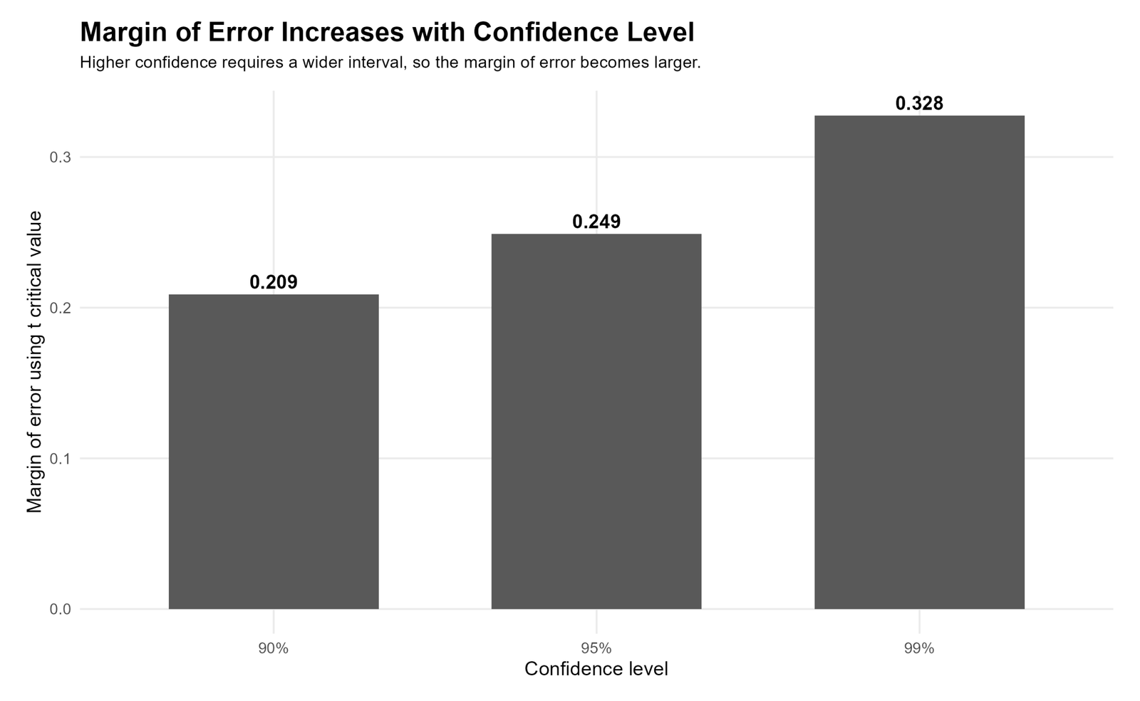
The R confidence-level chart confirms the expected pattern: 90% MOE = 0.209, 95% MOE = 0.249 and 99% MOE = 0.328. The chart visually teaches that higher confidence requires wider intervals. This is an important reporting point because readers often assume higher confidence is always better, but higher confidence reduces precision by increasing interval width.
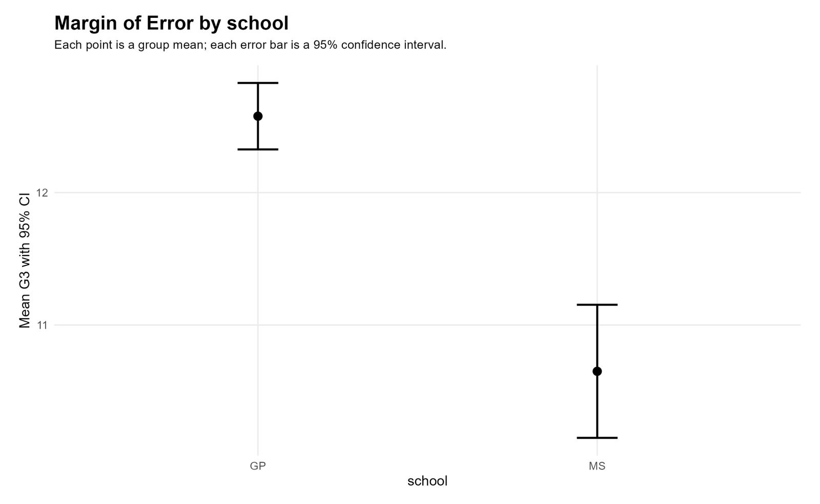
The R school chart validates the group pattern. GP has a higher average G3 score than MS, and the MS interval is wider. This happens because MS has fewer students and more score variability. The chart is useful for practical interpretation because it makes the precision difference visible: two groups can both have a mean estimate, but one estimate can be more uncertain than the other.

The R sample-size chart confirms the square-root relationship between sample size and margin of error. The curve falls quickly at first and then becomes flatter. This means very small samples are inefficient because they create wide intervals. Larger samples improve precision, but after a point, each additional case gives a smaller gain. This is why researchers plan sample size before collecting data.
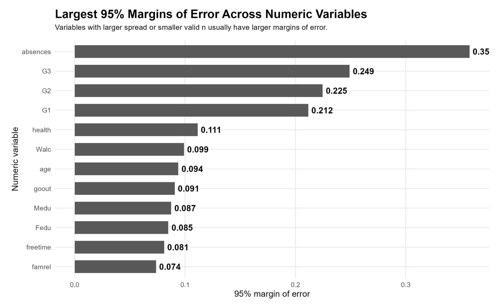
The R numeric-variable chart confirms that variables with larger spread have larger margins of error. Absences has the largest margin of error because it varies strongly across students. G3, G2 and G1 also have larger error margins than smaller-scale ordinal variables. This chart supports the practical rule that margin of error depends on both sample size and variability.
How to Calculate Margin of Error in Python, R, SPSS and Excel
Margin of Error in Python
Python can calculate standard error, t critical value, margin of error, confidence interval and a confidence-interval-based hypothesis decision.
import pandas as pd
import numpy as np
from scipy import stats

df = pd.read_csv("spss_ready_data.csv")
g3 = pd.to_numeric(df["G3"], errors="coerce").dropna()

n = len(g3)
mean_g3 = g3.mean()
sd_g3 = g3.std(ddof=1)
se_g3 = sd_g3 / np.sqrt(n)

confidence = 0.95
alpha = 1 - confidence
t_critical = stats.t.ppf(1 - alpha / 2, df=n - 1)

moe = t_critical * se_g3
lower_ci = mean_g3 - moe
upper_ci = mean_g3 + moe

# Hypothesis decision example: H0: mu = 12
mu0 = 12
t_stat = (mean_g3 - mu0) / se_g3
p_value = 2 * (1 - stats.t.cdf(abs(t_stat), df=n - 1))

print("N:", n)
print("Mean:", round(mean_g3, 4))
print("SD:", round(sd_g3, 4))
print("SE:", round(se_g3, 4))
print("t critical:", round(t_critical, 4))
print("95% margin of error:", round(moe, 4))
print("95% CI:", round(lower_ci, 4), "to", round(upper_ci, 4))
print("Null hypothesis: mu = 12")
print("Alternative hypothesis: mu != 12")
print("t statistic:", round(t_stat, 4))
print("p-value:", round(p_value, 4))

if lower_ci <= mu0 <= upper_ci:
    print("Decision: Fail to reject the null hypothesis.")
else:
    print("Decision: Reject the null hypothesis.")
Margin of Error in R
R can reproduce the same t-based margin of error and confidence interval.
student <- read.csv("spss_ready_data.csv")
g3 <- na.omit(as.numeric(student$G3))

n <- length(g3)
mean_g3 <- mean(g3)
sd_g3 <- sd(g3)
se_g3 <- sd_g3 / sqrt(n)

confidence <- 0.95
alpha <- 1 - confidence
t_critical <- qt(1 - alpha / 2, df = n - 1)

moe <- t_critical * se_g3
lower_ci <- mean_g3 - moe
upper_ci <- mean_g3 + moe

# Hypothesis decision example: H0: mu = 12
mu0 <- 12
t_stat <- (mean_g3 - mu0) / se_g3
p_value <- 2 * (1 - pt(abs(t_stat), df = n - 1))

cat("N:", n, "\n")
cat("Mean:", round(mean_g3, 4), "\n")
cat("SD:", round(sd_g3, 4), "\n")
cat("SE:", round(se_g3, 4), "\n")
cat("t critical:", round(t_critical, 4), "\n")
cat("95% margin of error:", round(moe, 4), "\n")
cat("95% CI:", round(lower_ci, 4), "to", round(upper_ci, 4), "\n")
cat("Null hypothesis: mu = 12\n")
cat("Alternative hypothesis: mu != 12\n")
cat("t statistic:", round(t_stat, 4), "\n")
cat("p-value:", round(p_value, 4), "\n")

if (lower_ci <= mu0 && mu0 <= upper_ci) {
  cat("Decision: Fail to reject the null hypothesis.\n")
} else {
  cat("Decision: Reject the null hypothesis.\n")
}
Margin of Error in SPSS
SPSS provides the mean, standard error and confidence interval through DESCRIPTIVES and EXAMINE. The margin of error can be confirmed by subtracting the mean from the upper confidence limit or subtracting the lower limit from the mean.
* Margin of Error Analysis in SPSS.
* Null hypothesis example: population mean G3 = 12.
* Alternative hypothesis example: population mean G3 is not equal to 12.

SET UNICODE=ON.
SET DECIMAL=DOT.
SET PRINTBACK=OFF.
SET MPRINT=OFF.

GET DATA
 /TYPE=TXT
 /FILE="D:\DATA ANALYSIS\A Basic Descriptive Statistics Guides\Margin of Error\SPSS_Output\clean_data\spss_ready_data.csv"
 /ENCODING='UTF8'
 /DELCASE=LINE
 /DELIMITERS=","
 /QUALIFIER='"'
 /ARRANGEMENT=DELIMITED
 /FIRSTCASE=2
 /IMPORTCASE=ALL.

DATASET NAME StudentData WINDOW=FRONT.

TITLE "Margin of Error Analysis for G3 Final Grade".

DESCRIPTIVES VARIABLES=G3
 /STATISTICS=MEAN STDDEV MIN MAX.

EXAMINE VARIABLES=G3
 /PLOT BOXPLOT HISTOGRAM NPPLOT
 /COMPARE GROUPS
 /STATISTICS DESCRIPTIVES
 /CINTERVAL 95
 /MISSING LISTWISE
 /NOTOTAL.

MEANS TABLES=G3 BY school
 /CELLS=COUNT MEAN STDDEV SEMEAN.

MEANS TABLES=G3 BY sex
 /CELLS=COUNT MEAN STDDEV SEMEAN.

OUTPUT EXPORT
 /CONTENTS EXPORT=VISIBLE
 /PDF DOCUMENTFILE="D:\DATA ANALYSIS\A Basic Descriptive Statistics Guides\Margin of Error\SPSS_Output\Margin-of-Error-SPSS-Output.pdf".
Margin of Error in Excel
Excel can calculate the standard error, t critical value, margin of error and confidence interval using formulas.
| Excel task | Example formula | Purpose |
|---|---|---|
| Sample size | =COUNT(B2:B650) | Counts valid G3 scores. |
| Mean | =AVERAGE(B2:B650) | Calculates the sample mean. |
| Standard deviation | =STDEV.S(B2:B650) | Calculates the sample standard deviation. |
| Standard error | =STDEV.S(B2:B650)/SQRT(COUNT(B2:B650)) | Calculates the standard error of the mean. |
| t critical value | =T.INV.2T(0.05,COUNT(B2:B650)-1) | Finds the two-sided 95% t critical value. |
| Margin of error | =T.INV.2T(0.05,COUNT(B2:B650)-1)*(STDEV.S(B2:B650)/SQRT(COUNT(B2:B650))) | Calculates the 95% margin of error. |
| Lower CI | =AVERAGE(B2:B650)-margin_error_cell | Calculates the lower confidence limit. |
| Upper CI | =AVERAGE(B2:B650)+margin_error_cell | Calculates the upper confidence limit. |
How to Report Margin of Error
A strong margin of error report should include the sample size, mean, standard deviation, standard error, confidence level, critical value, margin of error, confidence interval and any hypothesis decision based on a comparison value.
APA-style report: A 95% confidence interval was calculated for G3 final grade using 649 valid cases. The sample mean was 11.9060, with SD = 3.2307 and SE = 0.1268. Using a t critical value of 1.9636, the 95% margin of error was 0.2490, giving a 95% confidence interval of [11.6570, 12.1550]. Using 12 as a comparison value, the null hypothesis H0: μ = 12 was not rejected because 12 fell inside the confidence interval.
Plain-language report: The average final grade was about 11.91. The 95% margin of error was about 0.25, meaning the population average is likely between about 11.66 and 12.16. Since 12 is inside this range, the result does not show a clear difference from 12.
When reporting margin of error, it is also useful to explain why the interval is wide or narrow. Wider intervals can come from smaller sample sizes, larger standard deviations or higher confidence levels. Narrower intervals can come from larger samples, smaller variation or lower confidence levels. Related reporting topics include confidence interval, effect size, coefficient of variation and descriptive statistics.
Common Mistakes
1. Confusing margin of error with standard error
Standard error is the uncertainty of the sample mean. Margin of error is the standard error multiplied by a critical value. In this example, the standard error is about 0.1268, while the 95% margin of error is about 0.2490.
2. Forgetting to state the confidence level
A margin of error is incomplete without a confidence level. The same data can have different margins of error at 90%, 95% and 99% confidence levels.
3. Reporting the interval without the hypothesis decision
If a comparison value is being tested, state the null hypothesis and alternative hypothesis. Then explain whether the comparison value is inside or outside the confidence interval.
4. Saying higher confidence means better precision
Higher confidence gives a wider interval, not a more precise estimate. The 99% margin of error is larger than the 95% margin of error.
5. Ignoring sample size
Margin of error decreases as sample size increases, but the improvement follows the square-root rule. Doubling the sample size does not cut the margin of error in half.
6. Ignoring variable spread
Variables with larger standard deviations usually have larger margins of error. That is why absences has a larger margin of error than many smaller-scale ordinal variables.
Download SPSS Output and Verification Files
The SPSS output PDF verifies the descriptive statistics, standard error, confidence interval, normality checks, histogram, Q-Q plot, boxplot and group means used in this guide.
External References for Margin of Error
This post uses verified Python, R and SPSS outputs together with standard statistical documentation and dataset references.
FAQs About Margin of Error
What is margin of error?
Margin of error is the amount added to and subtracted from a sample estimate to create a confidence interval. It shows the likely uncertainty around the estimate.
What is the margin of error formula?
The formula is margin of error = critical value × standard error. For a mean, standard error is usually calculated as sample standard deviation divided by the square root of sample size.
How do you calculate margin of error for a mean?
Calculate the sample mean, standard deviation, sample size, standard error and critical value. Then multiply the standard error by the critical value.
What was the 95% margin of error for G3?
The 95% t-based margin of error for G3 final grade was approximately 0.2490.
What was the 95% confidence interval for G3?
The 95% confidence interval for the G3 mean was approximately 11.6570 to 12.1550.
What is the null hypothesis for this margin of error example?
The example null hypothesis is H0: μ = 12, meaning the population mean G3 final grade equals 12.
What is the alternative hypothesis for this example?
The alternative hypothesis is H1: μ ≠ 12, meaning the population mean G3 final grade differs from 12.
What was the hypothesis decision?
Because 12 lies inside the 95% confidence interval, we fail to reject the null hypothesis that the population mean equals 12.
Is margin of error the same as standard error?
No. Standard error measures uncertainty of the estimate. Margin of error multiplies standard error by a critical value to create a confidence interval.
Does margin of error increase with confidence level?
Yes. A higher confidence level uses a larger critical value, so the margin of error becomes larger and the interval becomes wider.
Does margin of error decrease with sample size?
Yes. As sample size increases, standard error decreases, so margin of error usually becomes smaller.
How do I calculate margin of error in Excel?
Use the formula =T.INV.2T(alpha,n-1)*(STDEV.S(range)/SQRT(COUNT(range))) for a t-based margin of error.

