
Distribution Shape, Positive Skewness, Negative Skewness, SPSS, Python, R and Excel
Skewness: Formula, Interpretation, SPSS, Python, R and Excel Guide
Skewness measures the direction and degree of asymmetry in a distribution. A distribution can show positive skewness, negative skewness, right skewness, left skewness, or near-zero skewness. This complete guide explains Skewness with verified SPSS output, Python charts, R validation charts, Excel workflow, formula, test of skew, APA reporting, common mistakes, related normality checks, and downloadable resources.
Quick Answer: Skewness Result
The main SPSS result for G3 final grade showed Skewness = -0.913, Standard Error of Skewness = 0.096, Mean = 11.91, Median = 12.00, Mode = 11, SD = 3.231, and N = 649. Since the skewness value is negative, the skewness of the distribution is left skewness. This means the left tail is longer or more extreme than the right tail, and some low G3 values pull the distribution toward the lower end.
The test of skew can be summarized with a z-style check: Skewness / Standard Error of Skewness = -0.913 / 0.096 ≈ -9.51. This is far beyond the common ±1.96 reference rule, so the G3 distribution is not perfectly symmetric. The practical conclusion is that G3 has meaningful negative skewness, while absences has strong positive skewness.
Final interpretation: The G3 distribution shows negative skewness or left skewness. The left tail is influenced by unusually low final grades, including zero scores. The mean is slightly below the median, which is consistent with a left-skewed distribution. This result should be reported with histogram, boxplot, and skewness table evidence rather than relying on the skewness number alone.
Table of Contents
- What Is Skewness?
- Skewness Formula and Interpretation
- Positive Skewness, Negative Skewness, Right and Left Skewness
- Test of Skew and Hypothesis Context
- Dataset and Variables Used
- Verified SPSS Output Interpretation
- Skewness and Kurtosis Together
- Python Chart-by-Chart Interpretation
- R Chart-by-Chart Validation
- SPSS, R, Python and Excel Workflows
- Code Blocks for Skewness
- APA Reporting Wording
- Common Mistakes
- When to Use Skewness
- Downloads and Resources
- Related Guides
- FAQs
What Is Skewness?
Skewness is a descriptive statistic that measures the asymmetry of a distribution. A perfectly symmetric distribution has skewness close to zero. If the tail extends to the right, the distribution has positive skewness. If the tail extends to the left, the distribution has negative skewness or left skewness.
In practical reporting, Skewness helps answer questions such as: Is the distribution balanced around the center? Are there extreme low values or high values? Is the mean pulled away from the median? Does the shape suggest that normality checks are needed before using parametric tests?
Simple definition: Skewness tells whether the distribution has a longer tail on the left side or the right side.
For example, the G3 final grade distribution has Skewness = -0.913. This means the shape has left skewness. In contrast, absences has Skewness = 2.021, which means it has strong positive skewness or right skewness. The two variables show different types of asymmetry, so they should not be interpreted with the same shape description.
Skewness is often used with normality guides such as the Q-Q plot normality check, P-P plot normality check, Kolmogorov-Smirnov test, Lilliefors test, D’Agostino-Pearson test, and Cramer-von Mises test.
Skewness Formula and Interpretation
The sample Skewness formula compares each observation with the mean, raises the standardized difference to the third power, and averages the result. A simplified expression is:
The third power is important because it preserves direction. Values above the mean contribute positive cubic values. Values below the mean contribute negative cubic values. If the right tail is stronger, skewness becomes positive. If the left tail is stronger, skewness becomes negative.
| Skewness Value | Shape Name | Mean and Median Pattern | Interpretation |
|---|---|---|---|
| Near 0 | Approximately symmetric | Mean and median are close | The distribution is fairly balanced. |
| Positive | Positive skewness / right skewness | Mean often greater than median | Right tail is longer or more extreme. |
| Negative | Negative skewness / left skewness | Mean often less than median | Left tail is longer or more extreme. |
| Large absolute value | Strong asymmetry | Mean may be pulled from median | Use charts and normality checks before parametric interpretation. |
Skewness z Statistic
SPSS reports Skewness and the Standard Error of Skewness. A common quick check divides skewness by its standard error:
For G3, the result is:
z_skewness = -0.913 / 0.096
z_skewness ≈ -9.51
This indicates clear asymmetry. However, with large samples, even small deviations from symmetry can become statistically noticeable. Therefore, always combine the test of skew with histograms, boxplots, mean-median comparison and practical judgment.
Positive Skewness, Negative Skewness, Right and Left Skewness
The phrases positive or negative skewness, right and left skewness, and skewness positive negative all describe the direction of the long tail. These terms are often confusing because “right skewness” and “positive skewness” mean the same thing, while “left skewness” and “negative skewness” mean the same thing.
| Common Name | Technical Name | Tail Direction | Typical Mean-Median Pattern | Example in This Guide |
|---|---|---|---|---|
| Right skewness | Positive skewness | Longer right tail | Mean often above median | Absences, skewness = 2.021 |
| Left skewness | Negative skewness | Longer left tail | Mean often below median | G3, skewness = -0.913 |
| Nearly symmetric | Near-zero skewness | No strong long tail | Mean and median close | G1, skewness = -0.003 |
Important: Do not decide skewness only by looking at whether the mean is above or below the median. Mean-median comparison is useful, but the full distribution, boxplot, outliers and SPSS skewness value should also be reviewed.
Test of Skew and Hypothesis Context
Skewness is primarily descriptive, but the test of skew can be explained with a hypothesis-style decision. This is helpful when reporting normality screening and distribution shape.
| Statement | Rule | Meaning |
|---|---|---|
| Null shape assumption | H0: Skewness = 0 | The distribution is symmetric in terms of skewness. |
| Alternative shape assumption | H1: Skewness ≠ 0 | The distribution has meaningful asymmetry. |
| Quick z rule | |Skewness / SE| > 1.96 | Skewness is noticeably different from zero at a rough 5% rule. |
Decision for G3: The G3 skewness z-style value is approximately -9.51. This is far beyond ±1.96, so the distribution is not symmetric. The practical conclusion is negative skewness or left skewness.
For formal normality decisions, do not rely on skewness alone. Use distribution charts and normality tools such as the Q-Q plot normality check 2, Kolmogorov-Smirnov test, Lilliefors test, and D’Agostino-Pearson test.
Dataset and Variables Used
The worked example uses the student performance dataset. The main variable is G3 final grade. Other numeric variables such as G1, G2, age and absences are included to compare Skewness across variables. This makes the guide stronger because it shows that not all variables have the same direction or degree of asymmetry.
| Variable | Role | Why It Matters for Skewness |
|---|---|---|
| G3 final grade | Main outcome variable | Used for the main skewness interpretation and chart explanation. |
| G1 | Previous grade variable | Shows near-zero skewness and provides a comparison with G3. |
| G2 | Previous grade variable | Shows mild negative skewness. |
| age | Background variable | Shows mild positive skewness. |
| absences | Count variable | Shows strong positive skewness with a long right tail. |
Before interpreting skewness, review distribution basics using descriptive statistics, frequency distribution, histogram interpretation, box plot interpretation, and five-number summary.
Verified SPSS Output Interpretation
The SPSS output verifies the Skewness values, standard errors, descriptive statistics, and related kurtosis values. The key result is that G3 has negative skewness, while absences has strong positive skewness. This comparison is important because it shows how different variables can have different distribution shapes in the same dataset.
Main SPSS Descriptive Table
| Variable | N | Mean | Median | SD | Skewness | SE Skewness | Kurtosis | Shape Interpretation |
|---|---|---|---|---|---|---|---|---|
| G1 | 649 | 11.40 | 11.00 | 2.745 | -0.003 | 0.096 | 0.037 | Approximately symmetric. |
| G2 | 649 | 11.57 | 11.00 | 2.914 | -0.360 | 0.096 | 1.662 | Mild negative skewness. |
| G3 | 649 | 11.91 | 12.00 | 3.231 | -0.913 | 0.096 | 2.712 | Clear left skewness. |
| age | 649 | 16.74 | 17.00 | 1.218 | 0.417 | 0.096 | 0.072 | Mild positive skewness. |
| absences | 649 | 3.66 | 2.00 | 4.641 | 2.021 | 0.096 | 5.781 | Strong positive skewness. |
Detailed G3 Interpretation
For G3, SPSS reported Skewness = -0.913. Because the sign is negative, the distribution has left skewness. The mean is 11.91, while the median is 12.00. The mean is slightly lower than the median, which is consistent with the negative skewness result. The G3 distribution is affected by unusually low scores, including zero values, which extend the left tail.
The G3 Standard Error of Skewness is 0.096. Dividing -0.913 by 0.096 gives a z-style value of about -9.51. This indicates that the skewness is not trivial. However, the practical interpretation should still be based on charts and context, not only the z-style statistic.
SPSS Decision Summary
| Decision Item | G3 Result | Interpretation |
|---|---|---|
| Skewness sign | Negative | Distribution has left skewness. |
| Skewness size | -0.913 | Meaningful asymmetry rather than near-zero symmetry. |
| Mean vs median | Mean 11.91, median 12.00 | Mean is slightly pulled downward by low values. |
| Skewness z-style check | -9.51 | Skewness is clearly different from zero under the quick rule. |
| Reporting decision | Left-skewed G3 distribution | Report skewness with histogram and boxplot support. |
Skewness and Kurtosis Together
Skewness and kurtosis are often reported together because they describe different parts of distribution shape. Skewness describes asymmetry and tail direction. Kurtosis describes tail heaviness or peakedness relative to a normal distribution. In the SPSS output, G3 has Skewness = -0.913 and Kurtosis = 2.712. This means G3 is left-skewed and also has a heavier or sharper tail pattern than a normal distribution under the SPSS excess-kurtosis style.
The phrase kurtosis and skewness is common in normality reporting. If both values are close to zero, the distribution may be closer to normal shape. If either value is large, charts and normality tests should be reviewed. For more detailed kurtosis interpretation, connect this post with your kurtosis guide and normality guides such as Q-Q plot normality check and P-P plot normality check.
Practical rule: Use skewness to describe direction of asymmetry and kurtosis to describe tail heaviness. Do not use one as a substitute for the other.
Python Chart-by-Chart Interpretation
The Python charts show the main Skewness interpretation visually. The charts include the G3 distribution with mean and median, skewness comparison across variables, boxplots with long tails, and mean-minus-median comparison. These charts are essential because skewness should be interpreted visually, not only numerically.
Python Chart 1: Distribution with Mean and Median
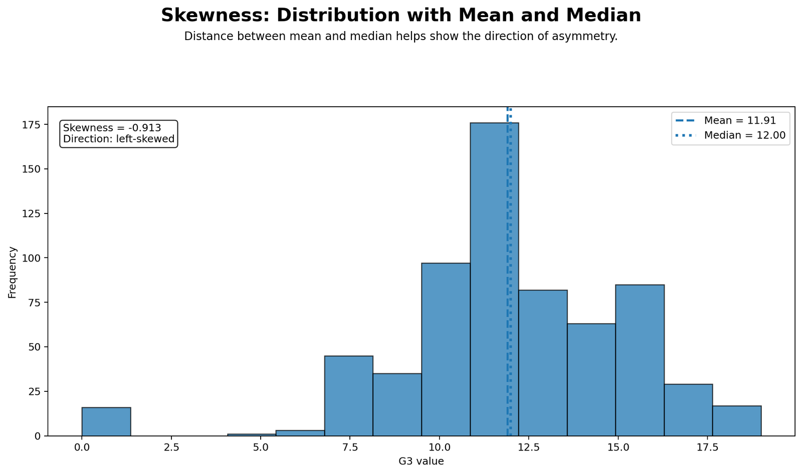
This chart shows the skewness of the distribution for G3. The histogram displays the grade pattern, while the mean and median lines help explain the direction of skewness. In a left-skewed distribution, low-end values pull the mean downward. In the G3 result, the mean is slightly below the median, which supports the SPSS result of negative skewness.
The distribution does not look perfectly symmetric because some low scores stretch the left side of the distribution. This is why the G3 skewness value is negative. The chart is useful for readers because it shows why the number -0.913 has a real shape meaning rather than being just a table value.
Python Chart 2: Skewness Comparison Across Variables
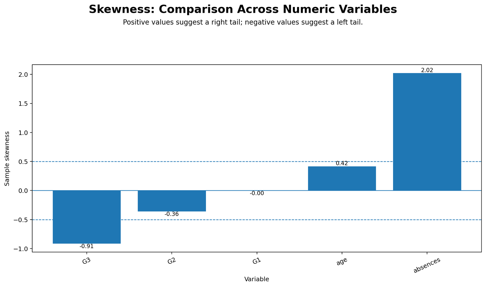
This chart compares Skewness across variables. G1 is almost symmetric, G2 is mildly negative, G3 is clearly negative, age is mildly positive, and absences is strongly positive. This comparison is important because it shows that skewness is variable-specific. One dataset can contain both left-skewed and right-skewed variables.
Absences stands out because it has strong positive skewness. Most students have few absences, while a smaller number have many absences, creating a long right tail. G3 shows the opposite direction because very low grades create left-tail influence. This chart directly supports the keywords positive skewness, left skewness, right and left skewness, and positive or negative skewness.
Python Chart 3: Boxplots and Long Tails
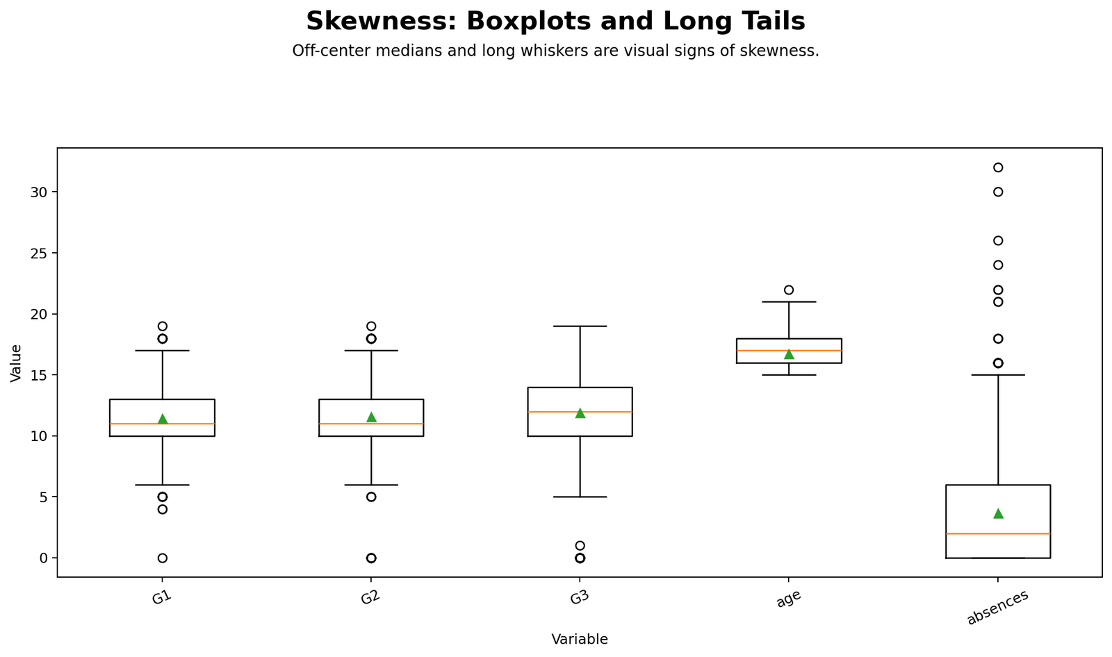
This chart explains skewness of box and whisker plots. A boxplot can show skewness through uneven whiskers, off-center median lines, and outliers concentrated on one side. For G3, the boxplot supports left-tail concern because unusually low values stretch the lower side. For absences, the boxplot supports right-tail concern because high absence values stretch the upper side.
This is why skewness box and whisker interpretation should not be skipped. A table may report a skewness number, but the boxplot shows the shape and outlier structure behind that number. When the whisker or outliers extend more strongly on one side, it visually supports positive or negative skewness.
Python Chart 4: Mean Minus Median
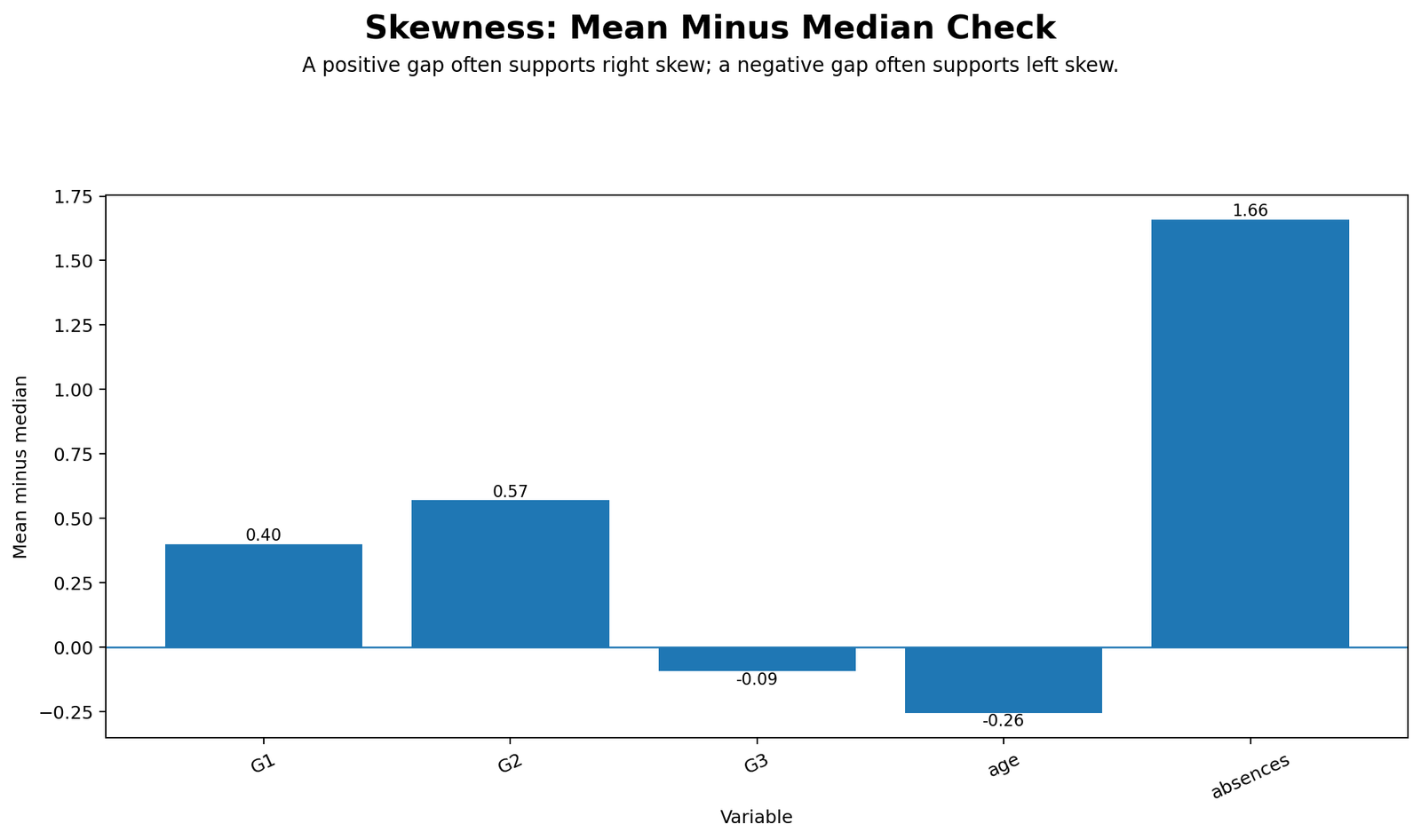
This chart uses mean minus median as a supporting shape indicator. When the mean is greater than the median, the distribution often has positive skewness. When the mean is less than the median, the distribution often has negative skewness. The chart does not replace the formal skewness value, but it helps readers understand why the mean and median positions matter.
For G3, the mean is slightly below the median, which is consistent with left skewness. For absences, the mean is above the median, which is consistent with positive skewness. This chart is useful for teaching because it links descriptive statistics with distribution shape.
R Chart-by-Chart Validation
The R charts validate the Python and SPSS Skewness interpretation using a separate workflow. The same pattern appears again: G3 is left-skewed, absences is right-skewed, and mean-median differences support the direction of asymmetry.
R Chart 1: Distribution with Mean and Median
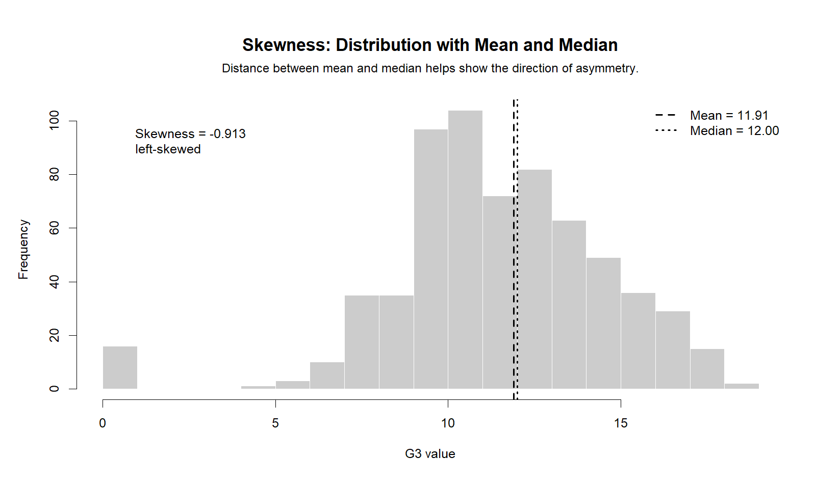
The R distribution chart confirms the Python chart. The G3 distribution is not perfectly symmetric, and the mean-median position supports a negative skewness interpretation. This validation is useful because it shows that the conclusion is not dependent on one software package.
The same reporting conclusion applies: G3 has left skewness. The distribution should be described as negatively skewed because low values extend the left side of the distribution.
R Chart 2: Skewness Comparison Across Variables
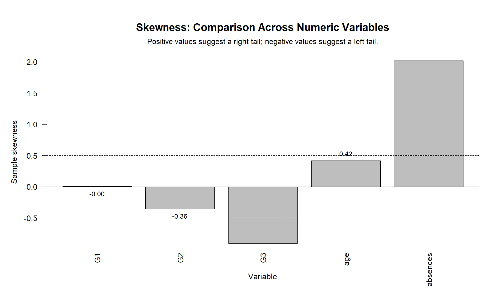
The R comparison chart confirms the variable-by-variable skewness pattern. G1 is almost symmetric, G2 has mild negative skewness, G3 has stronger negative skewness, age has mild positive skewness, and absences has strong positive skewness.
This chart supports the main statistical message: the researcher should not describe the whole dataset as skewed in one direction. Instead, each variable should be interpreted separately.
R Chart 3: Boxplots and Long Tails
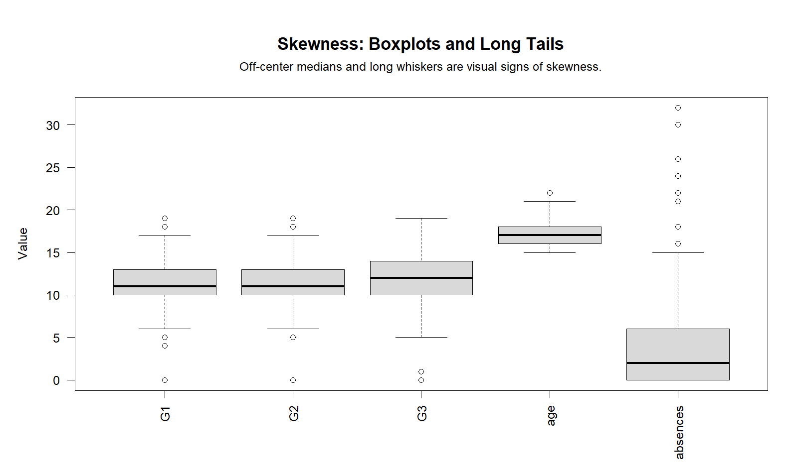
The R boxplot chart validates the skewness of box and whisker plots interpretation. It shows that tail direction and outliers are visible in boxplot form. Variables with long upper tails show positive skewness; variables with long lower tails show negative skewness.
This chart is useful for readers who prefer visual diagnostics. It also supports normality-check decisions because boxplot asymmetry can suggest the need for transformation, robust analysis or nonparametric methods.
R Chart 4: Mean Minus Median
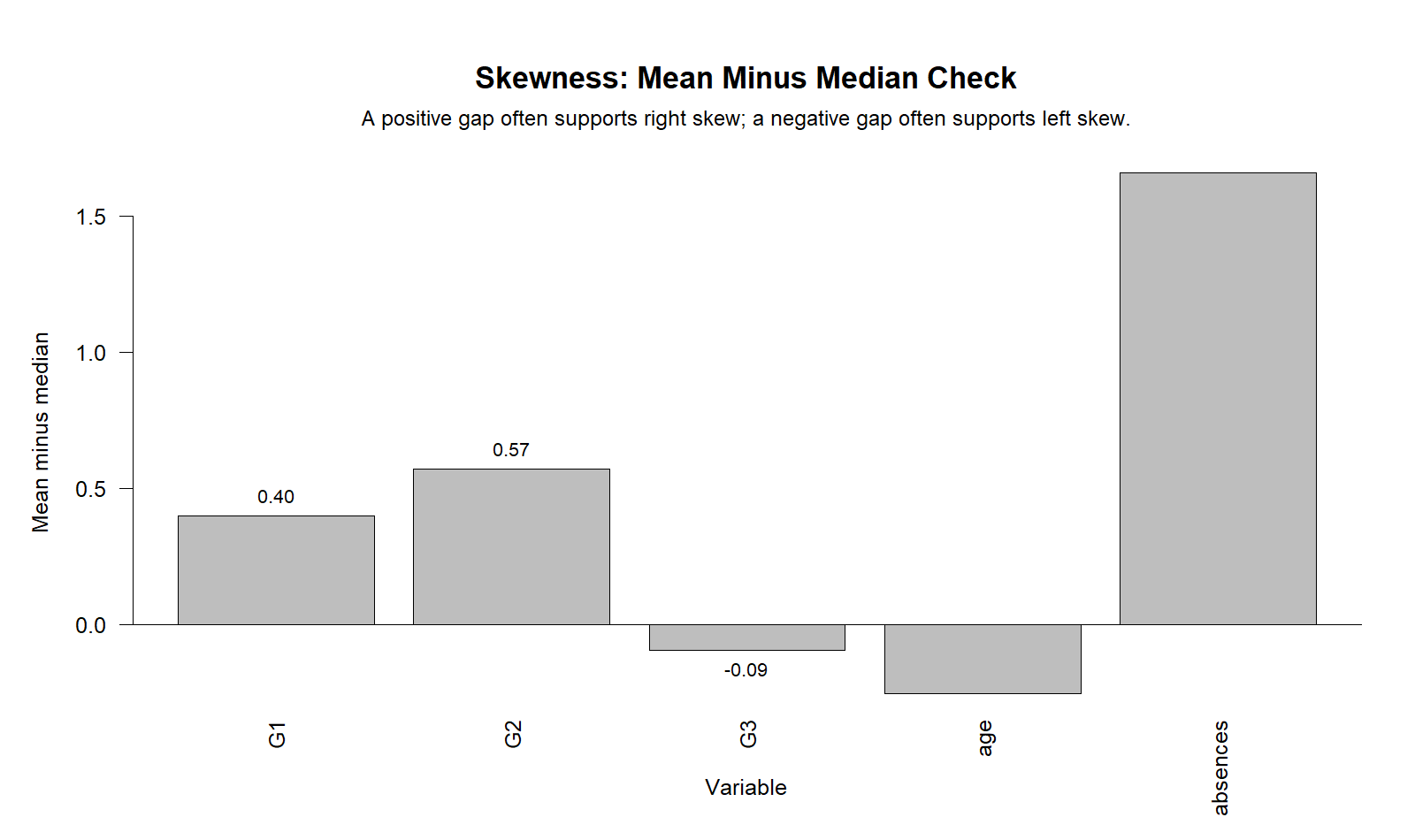
The R mean-minus-median chart confirms the Python result. The sign of mean minus median supports the direction of asymmetry. G3 has a mean slightly below the median, which supports negative skewness. Absences has a mean above the median, which supports positive skewness.
The correct conclusion is that mean-minus-median is a supporting diagnostic. It should be interpreted with the formal skewness value, histogram and boxplot.
SPSS, R, Python and Excel Workflows for Skewness
Skewness can be calculated in SPSS, R, Python and Excel. The workflow is similar in each tool: select numeric variables, calculate skewness, compare mean and median, inspect histograms and boxplots, and report whether the distribution shows positive skewness, negative skewness or approximate symmetry.
SPSS Workflow
| Step | SPSS Action | Purpose |
|---|---|---|
| Open dataset | File > Open > Data | Load the SPSS-ready dataset. |
| Run descriptives | Analyze > Descriptive Statistics > Frequencies or Descriptives | Request mean, median, skewness and standard error of skewness. |
| Run Explore | Analyze > Descriptive Statistics > Explore | Generate confidence intervals, plots and distribution diagnostics. |
| Read skewness sign | Skewness column | Identify positive skewness or negative skewness. |
| Check z-style statistic | Skewness / SE Skewness | Assess whether skewness is clearly different from zero. |
| Export output | File > Export or OUTPUT EXPORT | Save the SPSS PDF for reporting and verification. |
R Workflow
| Step | R Action | Purpose |
|---|---|---|
| Read data | read.csv() | Load the dataset into R. |
| Select numeric variables | c("G1","G2","G3","age","absences") | Choose variables for skewness comparison. |
| Calculate skewness | e1071::skewness() | Compute skewness values. |
| Compare center | mean() and median() | Support skewness direction using center measures. |
| Create charts | Base R or ggplot2 | Visualize distribution, boxplots and skewness comparison. |
Python Workflow
| Step | Python Action | Purpose |
|---|---|---|
| Read data | pandas.read_csv() | Load the dataset into a DataFrame. |
| Select variables | Choose numeric columns | Use the same variables as SPSS and R. |
| Calculate skewness | series.skew() or scipy.stats.skew() | Compute skewness values. |
| Calculate SE of skewness | sqrt(6/n) approximation | Support z-style skewness check. |
| Create charts | matplotlib | Build histogram, comparison, boxplot and mean-minus-median charts. |
Excel Workflow
| Excel Task | Formula or Tool | Purpose |
|---|---|---|
| Calculate mean | =AVERAGE(range) | Find the sample mean. |
| Calculate median | =MEDIAN(range) | Find the middle value. |
| Calculate standard deviation | =STDEV.S(range) | Measure spread. |
| Calculate skewness | =SKEW(range) | Compute sample skewness. |
| Create histogram | Insert > Statistical Chart > Histogram | Visualize distribution shape. |
| Create boxplot | Insert > Statistical Chart > Box and Whisker | Visualize tail direction and outliers. |
Code Blocks for Skewness
SPSS Syntax for Skewness
* Skewness analysis in SPSS.
* Main variable: G3 final grade.

TITLE "Skewness Descriptive Statistics".

FREQUENCIES VARIABLES=G1 G2 G3 age absences
  /STATISTICS=MEAN MEDIAN MODE STDDEV VARIANCE SKEWNESS SESKEW KURTOSIS SEKURT RANGE MINIMUM MAXIMUM
  /HISTOGRAM NORMAL
  /ORDER=ANALYSIS.

EXAMINE VARIABLES=G1 G2 G3 age absences
  /PLOT BOXPLOT HISTOGRAM NPPLOT
  /COMPARE GROUPS
  /STATISTICS DESCRIPTIVES
  /CINTERVAL 95
  /MISSING LISTWISE
  /NOTOTAL.

OUTPUT EXPORT
  /CONTENTS EXPORT=VISIBLE
  /PDF DOCUMENTFILE="Skewness-SPSS-Output.pdf".
Python Code for Skewness
import pandas as pd
import numpy as np
from scipy import stats

df = pd.read_csv("dataset.csv")

numeric_vars = ["G1", "G2", "G3", "age", "absences"]

rows = []
for col in numeric_vars:
    x = pd.to_numeric(df[col], errors="coerce").dropna()
    n = len(x)
    skew_value = stats.skew(x, bias=False)
    se_skew = np.sqrt(6 / n)
    z_skew = skew_value / se_skew

    rows.append({
        "variable": col,
        "n": n,
        "mean": x.mean(),
        "median": x.median(),
        "standard_deviation": x.std(ddof=1),
        "skewness": skew_value,
        "se_skewness": se_skew,
        "z_skewness": z_skew,
        "shape": "positive skewness" if skew_value > 0 else "negative skewness" if skew_value < 0 else "symmetric"
    })

skewness_table = pd.DataFrame(rows)
print(skewness_table)

# Main interpretation for G3
g3 = skewness_table[skewness_table["variable"] == "G3"].iloc[0]
print("G3 skewness:", g3["skewness"])
print("G3 z-style skewness:", g3["z_skewness"])
R Code for Skewness
# Skewness analysis in R

df <- read.csv("dataset.csv")

# install.packages("e1071")
library(e1071)

numeric_vars <- c("G1", "G2", "G3", "age", "absences")

rows <- lapply(numeric_vars, function(v) {
  x <- na.omit(as.numeric(df[[v]]))
  n <- length(x)
  skew_value <- skewness(x, type = 2)
  se_skew <- sqrt(6 / n)
  z_skew <- skew_value / se_skew

  data.frame(
    variable = v,
    n = n,
    mean = mean(x),
    median = median(x),
    standard_deviation = sd(x),
    skewness = skew_value,
    se_skewness = se_skew,
    z_skewness = z_skew,
    shape = ifelse(skew_value > 0, "positive skewness",
                   ifelse(skew_value < 0, "negative skewness", "symmetric"))
  )
})

skewness_table <- do.call(rbind, rows)
print(skewness_table)
Excel Formula Block for Skewness
Assume G3 values are in cells A2:A650.

Mean:
=AVERAGE(A2:A650)

Median:
=MEDIAN(A2:A650)

Standard deviation:
=STDEV.S(A2:A650)

Sample size:
=COUNT(A2:A650)

Skewness:
=SKEW(A2:A650)

Approximate standard error of skewness:
=SQRT(6/COUNT(A2:A650))

Skewness z statistic:
=SKEW(A2:A650)/SQRT(6/COUNT(A2:A650))

Interpretation:
If skewness > 0, positive skewness / right skewness.
If skewness < 0, negative skewness / left skewness.
If skewness is close to 0, approximate symmetry.
APA Reporting Wording for Skewness
When reporting Skewness, include the variable, sample size, skewness value, standard error of skewness if relevant, and shape interpretation. If skewness is used as part of a normality check, also mention the visual evidence from histogram, boxplot, Q-Q plot or P-P plot.
APA-Style Skewness Report
The distribution of G3 final grades showed negative skewness, skewness = -0.913, SEskewness = 0.096, indicating a left-skewed distribution. The mean score (M = 11.91) was slightly below the median (12.00), which supported the interpretation that low scores extended the left tail of the distribution.
Short Reporting Version
G3 final grades were negatively skewed, with Skewness = -0.913. This indicates left skewness, meaning the lower tail of the distribution was more extended than the upper tail.
Skewness and Kurtosis Reporting Version
Distribution shape was assessed using skewness and kurtosis. G3 showed negative skewness (skewness = -0.913) and positive kurtosis (kurtosis = 2.712), suggesting a left-skewed distribution with heavier tail behavior than a normal distribution.
Common Mistakes in Skewness Interpretation
| Mistake | Why It Is a Problem | Correct Practice |
|---|---|---|
| Calling negative skewness right skewness | Negative skewness means the long tail is on the left. | Use negative skewness and left skewness together. |
| Calling positive skewness left skewness | Positive skewness means the long tail is on the right. | Use positive skewness and right skewness together. |
| Using only mean and median | Mean-median comparison is only supporting evidence. | Use skewness value, histogram and boxplot. |
| Ignoring outliers | Outliers can strongly affect skewness. | Inspect boxplots and long tails. |
| Confusing skewness and kurtosis | Skewness measures asymmetry; kurtosis measures tail heaviness. | Report skewness and kurtosis separately. |
| Assuming all skewness breaks parametric tests | Sample size, robustness and test purpose matter. | Use normality checks, plots, transformations or robust methods as needed. |
Important warning: A statistically noticeable Skewness value does not automatically mean the analysis is invalid. It means distribution shape should be checked and reported carefully.
When to Use Skewness
Use Skewness when you need to describe distribution shape, check normality assumptions, compare variables, identify tail direction, understand mean-median differences, or decide whether transformations or nonparametric methods may be needed.
| Use Skewness When | Reason | Example from This Guide |
|---|---|---|
| Describing distribution shape | Skewness tells whether the distribution is symmetric or asymmetric. | G3 is left-skewed. |
| Checking normality | Strong skewness can indicate departure from normal shape. | G3 has skewness -0.913. |
| Comparing variables | Different variables can have different skewness directions. | G3 is negative; absences is positive. |
| Explaining boxplots | Long whiskers and outliers can show skewness visually. | Boxplots show long-tail direction. |
| Choosing transformations | Strong skewness may motivate transformation or robust analysis. | Absences may need special handling due to strong positive skewness. |
For transformations and assumption decisions, review related guides such as reciprocal transformation, central limit theorem, Levene’s test, Brown-Forsythe test, and effect size.
Downloads and Resources for Skewness
The SPSS output PDF below verifies the Skewness values, standard error of skewness, kurtosis, descriptive statistics, confidence intervals and supporting output used in this guide.
FAQs About Skewness
What is Skewness?
Skewness is a statistic that measures the asymmetry of a distribution. It tells whether the distribution has a longer tail on the right or on the left.
What does positive skewness mean?
Positive skewness means the distribution has a longer right tail. It is also called right skewness.
What does negative skewness mean?
Negative skewness means the distribution has a longer left tail. It is also called left skewness.
What was the skewness of G3 in this example?
The G3 variable had Skewness = -0.913, indicating negative skewness or left skewness.
What was the standard error of skewness for G3?
The SPSS output showed Standard Error of Skewness = 0.096 for G3.
How do I calculate a test of skew?
A common quick check divides skewness by the standard error of skewness. For G3, -0.913 / 0.096 ≈ -9.51.
Is skewness the same as kurtosis?
No. Skewness measures asymmetry and tail direction. Kurtosis measures tail heaviness or peakedness.
How can I see skewness in a box and whisker plot?
Skewness of box and whisker plots can be seen through uneven whiskers, off-center medians and outliers concentrated on one side.
Can a variable have positive and negative skewness in the same dataset?
A single variable has one skewness value, but different variables in the same dataset can have different skewness directions. In this guide, G3 is negatively skewed while absences is positively skewed.
How do I calculate skewness in Excel?
Use =SKEW(range) to calculate sample skewness in Excel.
How do I calculate skewness in Python?
Use scipy.stats.skew() or pandas.Series.skew() to calculate skewness in Python.
How do I calculate skewness in R?
Use a package such as e1071 and the function skewness(), or calculate skewness manually from standardized deviations.
Does skewness prove non-normality?
Skewness is strong evidence about distribution shape, but formal normality interpretation should also use histograms, Q-Q plots, P-P plots and normality tests.
Should skewed data always be transformed?
No. Transformation depends on the analysis goal, model assumptions, sample size, outliers and interpretability. Skewness should be reviewed before deciding.

