
Repeated-Measures ANOVA, Sphericity Violation, Epsilon Correction and Corrected Degrees of Freedom
Greenhouse-Geisser Correction: Formula, Interpretation, SPSS, Python, R and Excel Guide
Greenhouse-Geisser Correction is used in repeated-measures ANOVA when the sphericity assumption is violated. It corrects the degrees of freedom with the Greenhouse-Geisser epsilon value, making the within-subjects F test safer and less likely to overstate significance. This guide explains Greenhouse-Geisser Correction with verified SPSS output, Python charts, R validation charts, Excel support workflow, corrected p-values, repeated-measures mean profiles, APA reporting wording, common mistakes, and downloadable resources from Salar Cafe.
Quick Answer: Greenhouse-Geisser Correction Result
The verified repeated-measures ANOVA used three repeated grade measurements: G1, G2, and G3. The within-subjects factor was Time with three levels. The means increased from G1 = 11.40 to G2 = 11.57 and G3 = 11.91. Because the same students were measured at all three grade points, the correct design is repeated-measures, not three separate independent groups.
The sphericity assumption was checked using Mauchly’s Test of Sphericity. SPSS reported Mauchly’s W = .827, χ²(2) = 122.814, and p < .001. Since the p-value is below .05, sphericity is violated. Therefore, the Greenhouse-Geisser corrected row should be used instead of the sphericity-assumed row.
Hypothesis-style decision: The repeated-measures Time effect tests whether the repeated grade means are equal. The null hypothesis is H0: μG1 = μG2 = μG3. The alternative hypothesis is H1: at least one Time mean is different. After Greenhouse-Geisser correction, the Time effect remains significant, F(1.705, 1104.961) = 36.287, p < .001, partial η² = .053. Therefore, reject the null hypothesis and conclude that the repeated grade means changed significantly across G1, G2 and G3.
Final interpretation: The Greenhouse-Geisser Correction was required because Mauchly’s Test showed a sphericity violation. After applying the correction, the repeated-measures Time effect was still statistically significant. This means student grade means changed significantly across G1, G2 and G3. The correction changed the degrees of freedom but did not change the overall conclusion.
Important note: Greenhouse-Geisser Correction is not a separate mean-comparison test. It is a correction to the repeated-measures ANOVA degrees of freedom after sphericity is violated. To build the full assumption-checking workflow, compare this guide with Mauchly’s Test of Sphericity, Effect Size, Confidence Interval, Levene Test, and Brown-Forsythe Test.
Table of Contents
- What Is Greenhouse-Geisser Correction?
- Greenhouse-Geisser Formula and Epsilon Logic
- Null and Alternative Hypotheses
- Dataset and Repeated Measures Used
- Verified SPSS Output Interpretation
- Python Chart-by-Chart Interpretation
- R Chart-by-Chart Validation
- SPSS, R, Python and Excel Workflows
- Code Blocks for Greenhouse-Geisser Correction
- APA Reporting Wording
- Common Mistakes
- When to Use Greenhouse-Geisser Correction
- Downloads and Resources
- Related Guides
- FAQs
What Is Greenhouse-Geisser Correction?
Greenhouse-Geisser Correction is a repeated-measures ANOVA correction used when the sphericity assumption is violated. Sphericity means that the variances of all pairwise difference scores among repeated-measure levels are equal. When sphericity is violated, the usual sphericity-assumed F test can be too liberal. The Greenhouse-Geisser Correction protects the analysis by reducing the degrees of freedom using an epsilon value.
In this guide, the repeated measurements are G1, G2, and G3. These represent three repeated grade measurements for the same students. Because there are three repeated levels, the sphericity assumption applies. SPSS reports Mauchly’s Test of Sphericity, which is significant in this example. Therefore, the correct repeated-measures ANOVA interpretation should use the Greenhouse-Geisser corrected row.
The Greenhouse-Geisser epsilon in the verified SPSS output is .853. An epsilon value closer to 1 means the sphericity violation is not extremely severe, while a lower epsilon means stronger correction. Here, the correction is meaningful but not extreme. The corrected Time effect remains significant with p < .001. When writing the final report, use the corrected F test together with effect size and confidence interval interpretation where appropriate.
Practical meaning: Greenhouse-Geisser Correction answers this question: “If sphericity is violated, what is the safer repeated-measures ANOVA result?” In this example, the safer corrected result still shows a significant Time effect.
Greenhouse-Geisser Formula and Epsilon Logic
The Greenhouse-Geisser Correction adjusts the degrees of freedom by multiplying them by the Greenhouse-Geisser epsilon value. The F statistic itself remains the same in SPSS, but the degrees of freedom and p-value are recalculated using the corrected degrees of freedom.
For the Time effect in this output, the original numerator degrees of freedom were 2. The Greenhouse-Geisser epsilon was .853. Therefore, the corrected numerator degrees of freedom became approximately:
The original error degrees of freedom were 1296. The corrected error degrees of freedom became approximately:
The corrected repeated-measures Time effect was then reported as:
| Correction Concept | Value in This Output | Interpretation |
|---|---|---|
| Mauchly’s Test | W = .827, p < .001 | Sphericity is violated, so correction is needed. |
| Greenhouse-Geisser epsilon | .853 | Corrects the degrees of freedom. |
| Huynh-Feldt epsilon | .855 | A less conservative correction with a similar conclusion. |
| Lower-bound epsilon | .500 | Most conservative correction for three repeated levels. |
| Corrected Time effect | F = 36.287, p < .001 | The repeated-measures Time effect remains significant. |
Formula caution: The Greenhouse-Geisser Correction does not change the repeated-measures means. It changes the degrees of freedom used to evaluate the F test. Therefore, the conclusion should report the corrected degrees of freedom, F statistic, p-value, epsilon, and effect size. For broader model-checking context, use Cochran C Test, Goldfeld-Quandt Test, and Ramsey RESET Test when your design requires those specific diagnostics.
Null and Alternative Hypotheses
The Greenhouse-Geisser Correction is used after a sphericity decision, but the repeated-measures ANOVA still tests the Time effect. For this guide, there are two useful hypothesis sections: one for sphericity and one for the corrected repeated-measures Time effect.
Sphericity Assumption Hypotheses
| Statement | Hypothesis | Decision in This Output |
|---|---|---|
| Sphericity null hypothesis | H0: sphericity is met | Rejected because Mauchly’s Test p < .001. |
| Sphericity alternative hypothesis | H1: sphericity is violated | Supported because Mauchly’s Test is significant. |
Corrected Repeated-Measures Time Effect Hypotheses
| Statement | Hypothesis | Decision in This Output |
|---|---|---|
| Time effect null hypothesis | H0: μG1 = μG2 = μG3 | Rejected because corrected p < .001. |
| Time effect alternative hypothesis | H1: at least one repeated mean differs | Supported because the corrected Time effect is significant. |
Hypothesis-style decision: First, Mauchly’s Test rejects the sphericity null hypothesis, so correction is needed. Second, the Greenhouse-Geisser corrected repeated-measures ANOVA rejects the Time-effect null hypothesis. Therefore, the final report should say that the Time effect was significant after Greenhouse-Geisser correction.
Related hypothesis-test note: If the analysis changes from repeated grades to one-sample, directional, or proportion-based questions, use the correct guide such as One Sample Z Test, One-Tailed T Test, or One Proportion Z Test. Greenhouse-Geisser Correction is specifically for repeated-measures ANOVA sphericity correction.
Dataset and Repeated Measures Used
The worked example uses three repeated grade variables from the same 649 students: G1, G2, and G3. SPSS defines a within-subjects factor named Time with three levels. Because the same students have all three grade measurements, this is a repeated-measures design.
| Repeated Measure | Time Level | N | Mean | Standard Deviation | Interpretation |
|---|---|---|---|---|---|
| G1 | Time 1 | 649 | 11.40 | 2.745 | First repeated grade measurement and lowest mean. |
| G2 | Time 2 | 649 | 11.57 | 2.914 | Second repeated grade measurement with a slight increase. |
| G3 | Time 3 | 649 | 11.91 | 3.231 | Final repeated grade measurement and highest mean. |
Before interpreting the repeated-measures model, it is useful to review descriptive summaries such as Descriptive Statistics, Frequency Distribution, Five Number Summary, Histogram Interpretation, Box Plot Interpretation, and Coefficient of Variation. These guides help explain the distribution and spread of G1, G2 and G3 before the repeated-measures ANOVA is reported.
Verified SPSS Output Interpretation
The SPSS output provides repeated-measures descriptives, Mauchly’s Test of Sphericity, epsilon values, uncorrected and corrected within-subjects effects, contrast tests, group context by sex, and homogeneity checks. The key reporting result is the Greenhouse-Geisser corrected Time effect.
SPSS Repeated-Measures Descriptive Statistics
| Measure | Mean | Standard Deviation | N | Interpretation |
|---|---|---|---|---|
| G1 | 11.40 | 2.745 | 649 | Lowest repeated-measures mean. |
| G2 | 11.57 | 2.914 | 649 | Mean increases slightly from G1. |
| G3 | 11.91 | 3.231 | 649 | Highest repeated-measures mean and largest SD. |
SPSS Mauchly’s Test and Epsilon Values
| Within-Subjects Effect | Mauchly’s W | Approx. Chi-Square | df | Sig. | Greenhouse-Geisser ε | Huynh-Feldt ε | Lower-bound ε |
|---|---|---|---|---|---|---|---|
| Time | .827 | 122.814 | 2 | p < .001 | .853 | .855 | .500 |
Mauchly’s Test is significant, so the sphericity assumption is violated. Because the Greenhouse-Geisser epsilon is .853, the degrees of freedom are reduced from the sphericity-assumed values to the corrected values. If you need the full assumption explanation, read Mauchly’s Test of Sphericity before reporting the corrected row.
SPSS Tests of Within-Subjects Effects
| Time Row | Type III SS | df | Mean Square | F | Sig. | Partial Eta Squared | Reporting Decision |
|---|---|---|---|---|---|---|---|
| Sphericity Assumed | 86.331 | 2 | 43.165 | 36.287 | p < .001 | .053 | Not the main row because sphericity was violated. |
| Greenhouse-Geisser | 86.331 | 1.705 | 50.628 | 36.287 | p < .001 | .053 | Main corrected row to report. |
| Huynh-Feldt | 86.331 | 1.709 | 50.509 | 36.287 | p < .001 | .053 | Alternative corrected row with nearly identical conclusion. |
| Lower-bound | 86.331 | 1.000 | 86.331 | 36.287 | p < .001 | .053 | Most conservative row; still significant. |
SPSS Within-Subjects Contrasts
| Contrast | Type III SS | df | F | Sig. | Partial Eta Squared | Interpretation |
|---|---|---|---|---|---|---|
| Time Linear | 83.391 | 1 | 50.309 | p < .001 | .072 | There is a significant upward linear grade trend. |
| Time Quadratic | 2.940 | 1 | 4.075 | .044 | .006 | There is a small quadratic pattern in the repeated profile. |
Group Context by Sex
| Group | N | G1 Mean | G2 Mean | G3 Mean | Profile Interpretation |
|---|---|---|---|---|---|
| Female | 383 | 11.64 | 11.82 | 12.25 | Female students show a rising mean grade profile. |
| Male | 266 | 11.06 | 11.21 | 11.41 | Male students also show a rising profile but lower means. |
Greenhouse-Geisser Group Model
| Effect | Greenhouse-Geisser df | F | Sig. | Partial Eta Squared | Interpretation |
|---|---|---|---|---|---|
| Time | 1.705, 1103.264 | 31.813 | p < .001 | .047 | The repeated-measures Time effect remains significant when sex is included. |
| Time × sex | 1.705, 1103.264 | 2.777 | .071 | .004 | The change pattern is not significantly different by sex after correction. |
If the repeated-measures analysis is later combined with categorical summaries, Cross Tabulation can help summarize group membership. For distribution-shape checks before modeling, use Q-Q Plot Normality Check, P-P Plot Normality Check, Kolmogorov-Smirnov Test, Lilliefors Test, D’Agostino-Pearson Test, Cramer-von Mises Test, and Ryan-Joiner Test.
SPSS interpretation summary: Mauchly’s Test was significant, so the sphericity-assumed row should not be the main result. The Greenhouse-Geisser corrected row shows that Time remains statistically significant, F(1.705, 1104.961) = 36.287, p < .001. In the group model, the Time effect remains significant, but the corrected Time × sex interaction is not significant.
Python Chart-by-Chart Interpretation
The Python charts visualize the Greenhouse-Geisser Correction workflow. They show the repeated-measures mean profile, individual spaghetti profiles, covariance heatmap, epsilon values, corrected p-values, pairwise difference boxplots, and group mean profiles.
Python Chart 1: Repeated-Measures Mean Profile
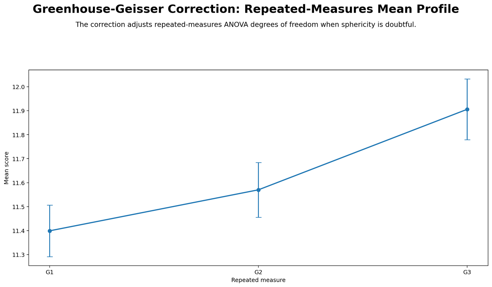
This chart shows the repeated-measures mean pattern. The average score increases from G1 = 11.40 to G2 = 11.57 and then to G3 = 11.91. This rising profile explains why the repeated-measures Time effect is statistically significant.
The chart shows the substantive mean trend, while the Greenhouse-Geisser Correction handles the assumption problem. Because Mauchly’s Test was significant, the mean profile should be interpreted with the corrected ANOVA row rather than only the sphericity-assumed row. For publication, pair the chart conclusion with Effect Size and Confidence Interval interpretation.
Python Chart 2: Individual Profiles Spaghetti Plot
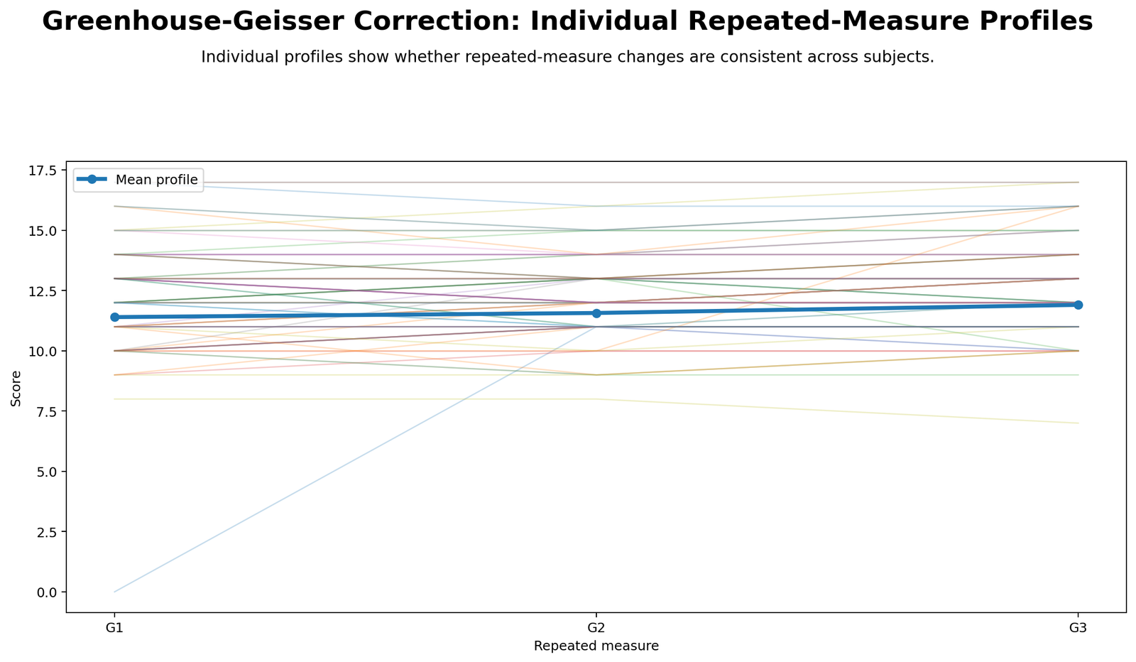
The spaghetti plot shows that individual students do not all follow exactly the same path across G1, G2 and G3. Some profiles rise, some stay similar, and some may decline. This individual variability is important because repeated-measures ANOVA depends on within-person change patterns.
The Greenhouse-Geisser Correction is relevant because repeated-measures data include dependence across time. The spaghetti plot makes that repeated structure visible and supports the need to treat the observations as related, not independent.
Python Chart 3: Repeated-Measure Covariance Heatmap
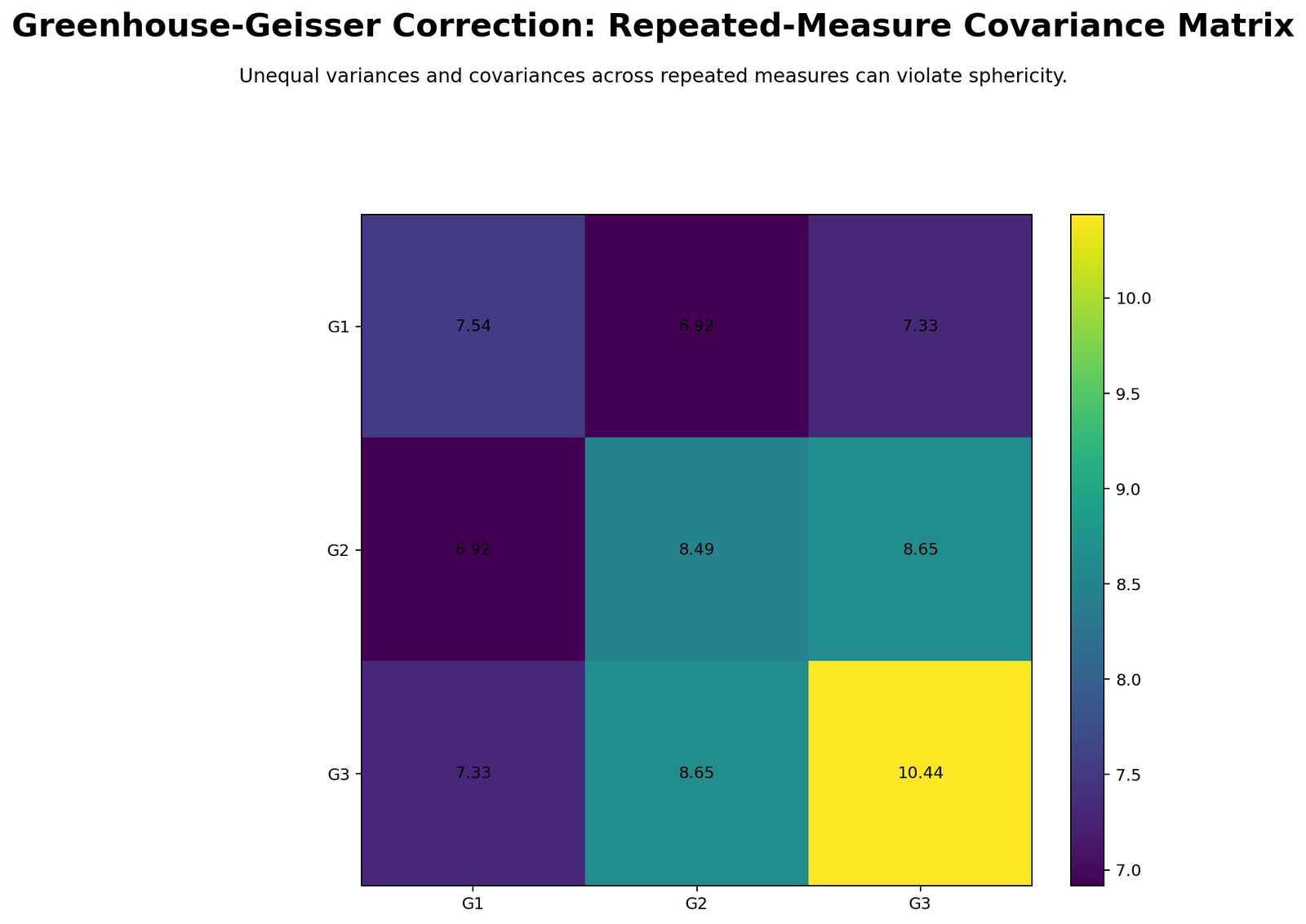
The covariance heatmap shows how G1, G2 and G3 are related. Repeated grades are expected to be strongly associated because they come from the same students and measure related academic performance. The correction is not based only on high correlations. It is needed when the sphericity structure is not adequate.
The heatmap helps explain the repeated-measures dependence, while Mauchly’s Test and epsilon values determine whether correction is needed. If your project is a regression-diagnostics project instead of repeated measures, a covariance or residual workflow may connect better with Ramsey RESET Test or Goldfeld-Quandt Test.
Python Chart 4: Epsilon Values
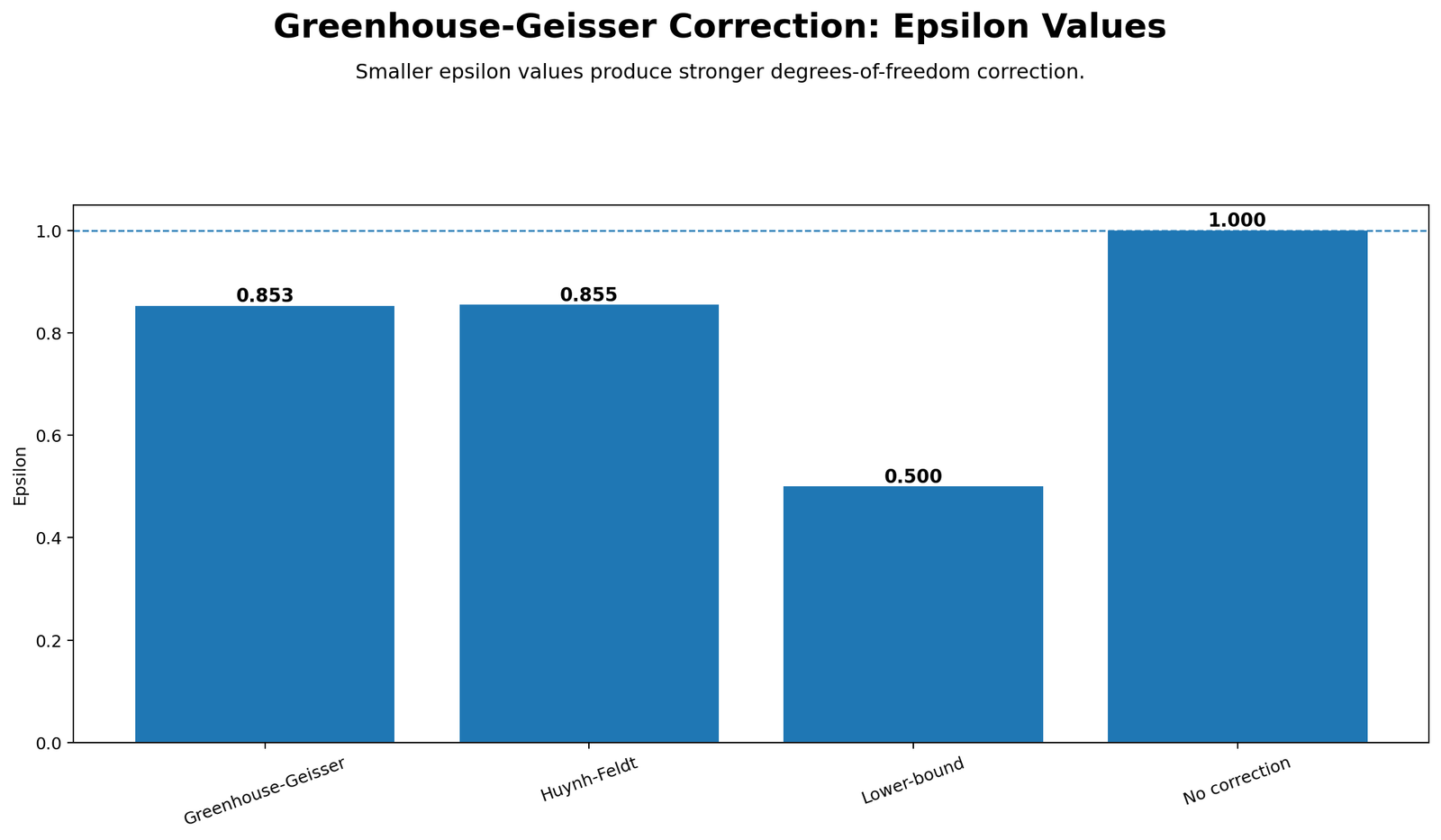
This chart shows the correction values. The Greenhouse-Geisser epsilon is .853, the Huynh-Feldt epsilon is about .855, and the lower-bound epsilon is .500. The Greenhouse-Geisser value is the main correction used in this guide.
Because ε = .853 is close to 1, the correction is moderate rather than severe. The corrected degrees of freedom are lower than the original degrees of freedom, but not dramatically lower. This explains why the corrected p-value remains significant.
Python Chart 5: Corrected p-values
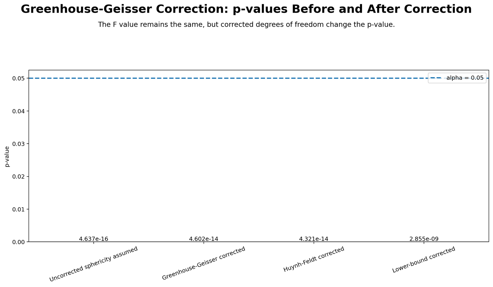
This chart compares the sphericity-assumed result with the Greenhouse-Geisser, Huynh-Feldt and lower-bound corrected results. In the verified output, the Time effect remains p < .001 under each correction method.
This is the main reporting conclusion: the correction changes the degrees of freedom but not the final decision. The grade means differ significantly across G1, G2 and G3 even after correcting for sphericity violation.
Python Chart 6: Pairwise Difference Boxplots
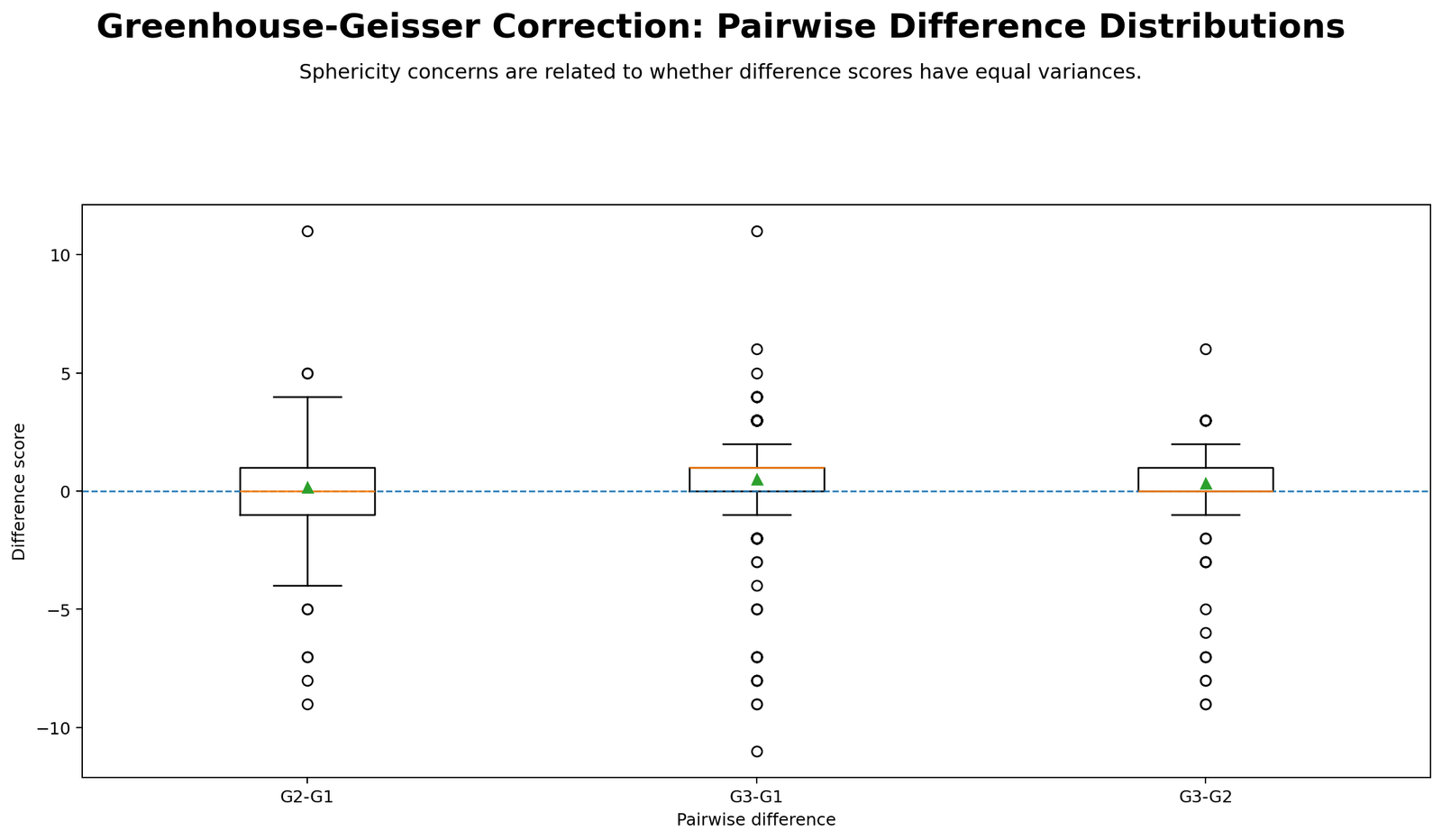
The pairwise difference boxplots help explain why the sphericity assumption matters. The differences between G2 and G1, G3 and G2, and G3 and G1 do not have identical spread. Unequal difference-score variances are the practical reason Mauchly’s Test can become significant.
This chart is useful for teaching because it connects the abstract correction to visible data behavior. The Greenhouse-Geisser Correction adjusts the ANOVA test after those difference-score patterns show that sphericity is not fully satisfied. If the analysis were instead about independent group variance equality, compare the logic with Levene Test, Brown-Forsythe Test, and Cochran C Test.
Python Chart 7: Group Mean Profiles
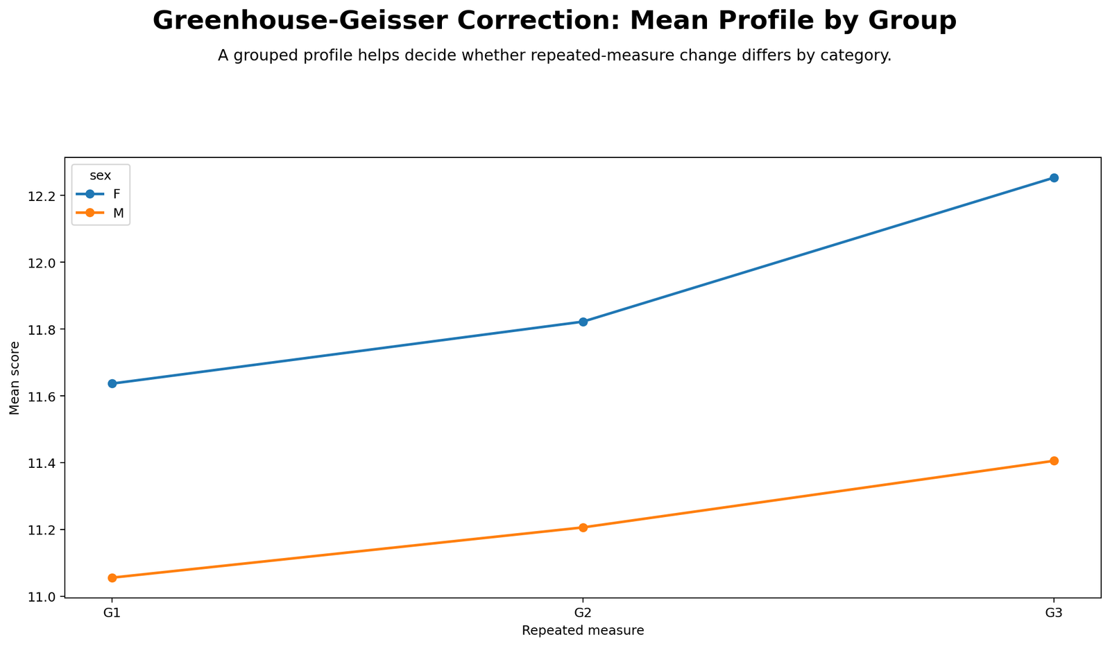
This chart compares repeated-measures mean profiles for female and male students. Female means are higher at each grade level, while both groups show an upward pattern from G1 to G3. Female means are 11.64, 11.82, and 12.25; male means are 11.06, 11.21, and 11.41.
SPSS shows that the corrected Time effect remains significant when sex is included, but the corrected Time × sex interaction is not significant at p = .071. This means the overall repeated profile changes, but the shape of change is not clearly different between female and male students after correction.
R Chart-by-Chart Validation
The R charts validate the same Greenhouse-Geisser Correction workflow using a separate software environment. They confirm the repeated-measures mean pattern, individual profile variability, covariance structure, epsilon correction values, corrected p-value decision, pairwise difference behavior, and group mean profile interpretation.
R Chart 1: Repeated-Measures Mean Profile
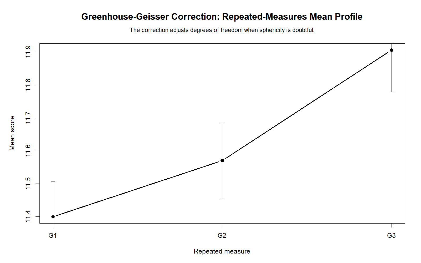
The R mean profile confirms the Python and SPSS pattern. Mean scores increase across the three repeated grade measures. This supports the significant corrected Time effect. It also confirms that the result is not software-specific.
R Chart 2: Individual Profiles Spaghetti Plot
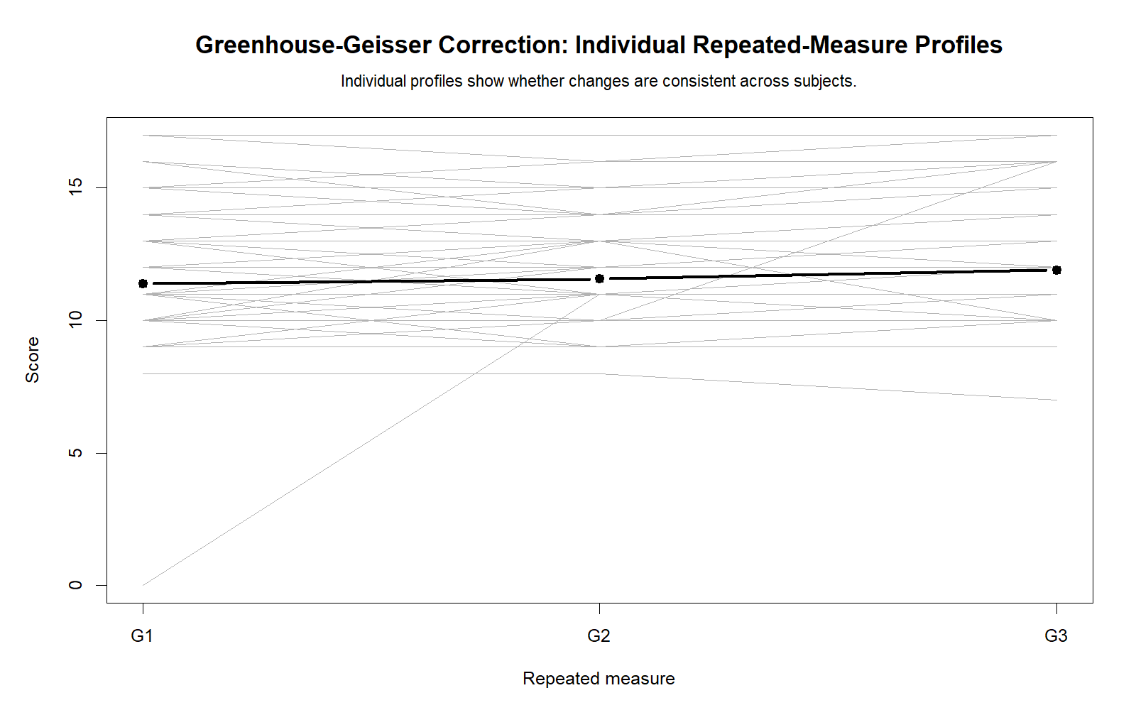
The R spaghetti plot validates the repeated-measures structure by showing within-student grade profiles. It confirms that the data should be analyzed as repeated observations rather than independent groups.
R Chart 3: Repeated-Measure Covariance Heatmap
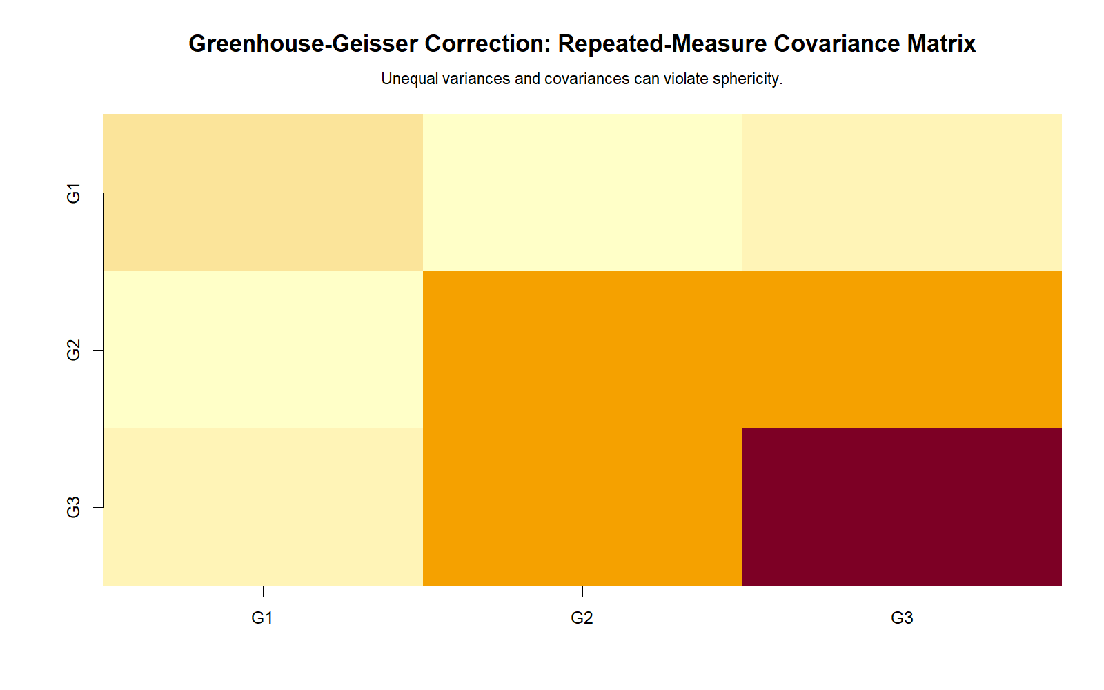
The R covariance heatmap confirms the repeated-measure dependence among G1, G2 and G3. The grade measures are strongly related, which is expected in a within-subjects design.
R Chart 4: Epsilon Values
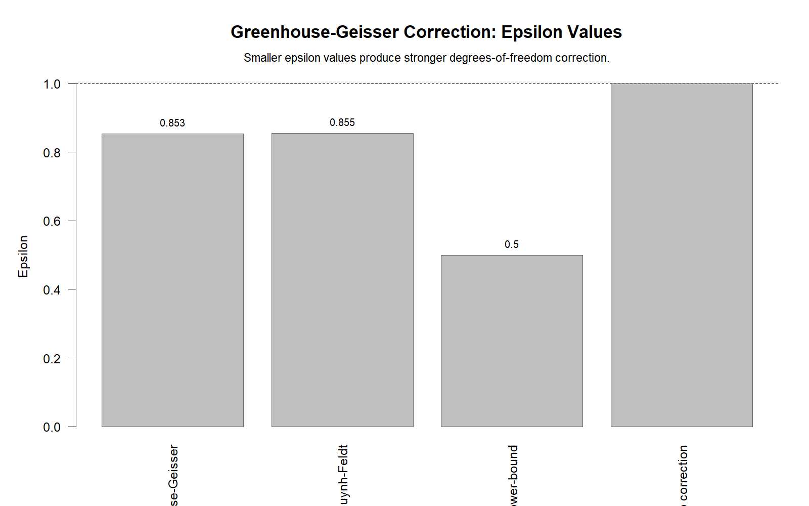
The R epsilon chart confirms the correction values. Greenhouse-Geisser epsilon is about .853, meaning corrected degrees of freedom should be used after the sphericity violation.
R Chart 5: Corrected p-values
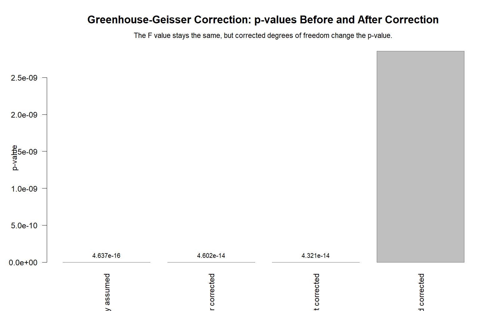
The R corrected p-value chart validates that the Time effect remains significant after correction. This confirms the SPSS interpretation and supports the final reporting conclusion.
R Chart 6: Pairwise Difference Boxplots
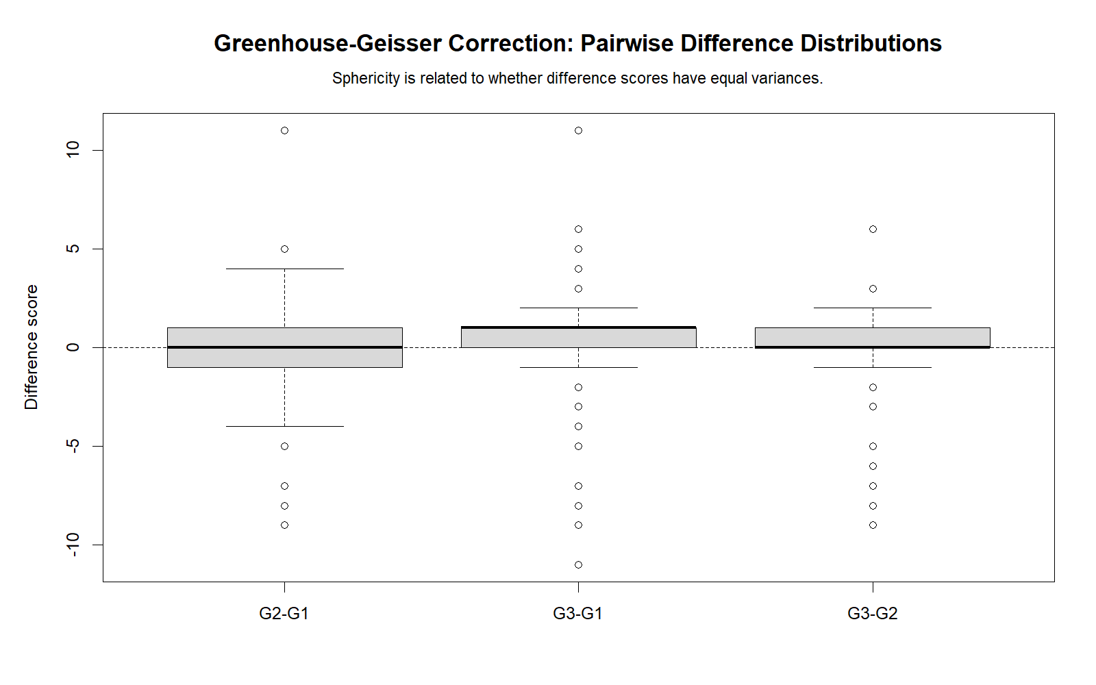
The R pairwise difference boxplots validate the sphericity context. Difference-score distributions are not identical, which supports the need to use the corrected repeated-measures result.
R Chart 7: Group Mean Profiles
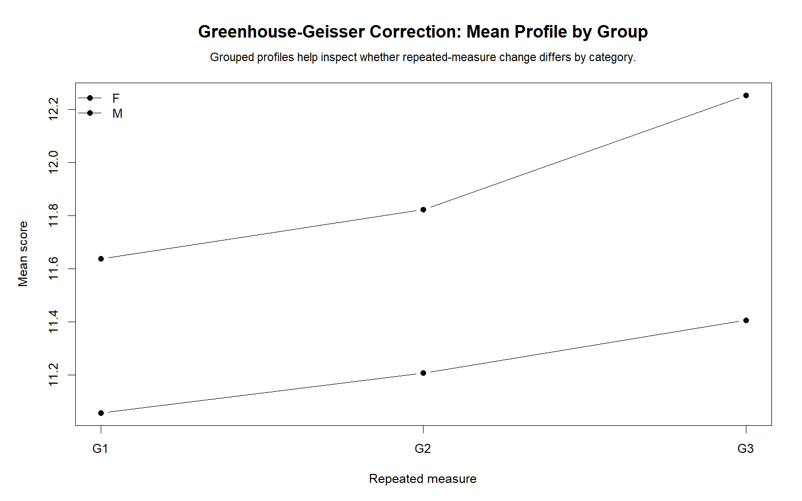
The R group profile chart confirms the same pattern as Python and SPSS. Female students have higher mean scores at each grade level, while both groups show a rising profile across G1, G2 and G3.
R validation conclusion: The R charts support the same substantive result as SPSS and Python. The grade profile rises over time, sphericity requires correction, and the corrected repeated-measures Time effect remains statistically significant.
SPSS, R, Python and Excel Workflows for Greenhouse-Geisser Correction
Greenhouse-Geisser Correction is usually applied by repeated-measures ANOVA software. SPSS reports it automatically when running repeated-measures GLM. R can report it through repeated-measures ANOVA packages. Python can calculate repeated-measures ANOVA and corrections through packages such as pingouin. Excel does not provide a direct Greenhouse-Geisser ANOVA row, but it can support interpretation by calculating difference scores, covariance matrices, mean profiles, and pairwise changes.
SPSS Workflow
| Step | SPSS Menu or Syntax | Purpose |
|---|---|---|
| Open dataset | File > Open > Data | Load the SPSS-ready dataset. |
| Define repeated-measures factor | Analyze > General Linear Model > Repeated Measures | Create Time with three levels. |
| Assign repeated variables | G1, G2, G3 | Place variables in correct time order. |
| Read Mauchly’s Test | Mauchly’s Test of Sphericity table | Check whether correction is needed. |
| Use corrected row | Tests of Within-Subjects Effects | Report Greenhouse-Geisser row when sphericity is violated. |
| Export output | File > Export or OUTPUT EXPORT | Save the SPSS output PDF. |
R Workflow
| Step | R Action | Purpose |
|---|---|---|
| Read data | read.csv() | Load wide-format repeated-measures data. |
| Add subject ID | id = row_number() | Identify the repeated observations for each student. |
| Convert to long format | pivot_longer() | Create Time and Score columns. |
| Run repeated-measures ANOVA | rstatix::anova_test() | Get sphericity test and Greenhouse-Geisser correction. |
| Plot profiles | ggplot2 | Create mean profiles and group profiles. |
Python Workflow
| Step | Python Action | Purpose |
|---|---|---|
| Read data | pandas.read_csv() | Load the dataset. |
| Add subject ID | np.arange() | Identify repeated rows for each student. |
| Convert to long format | pd.melt() | Create Time and Score columns. |
| Run sphericity test | pingouin.sphericity() | Check whether correction is needed. |
| Run repeated-measures ANOVA | pingouin.rm_anova() | Get corrected repeated-measures results. |
Excel Workflow
| Excel Task | Formula or Tool | Purpose |
|---|---|---|
| Mean of G1, G2, G3 | =AVERAGE(range) | Create repeated-measures mean profile. |
| Difference G2 − G1 | =B2-A2 | Create first pairwise difference. |
| Difference G3 − G2 | =C2-B2 | Create second pairwise difference. |
| Difference G3 − G1 | =C2-A2 | Create long-span difference. |
| Difference variance | =VAR.S(range) | Support sphericity interpretation. |
| Profile chart | Line chart | Visualize repeated-measures change. |
For complete applied reporting, the workflow should not stop at the corrected p-value. Use Descriptive Statistics for the means and spread, Effect Size for magnitude, Confidence Interval for estimation, and Clinical Trial Data Analysis Using R if your repeated-measures structure comes from a medical or experimental study design.
Code Blocks for Greenhouse-Geisser Correction
SPSS Syntax for Greenhouse-Geisser Correction
* Greenhouse-Geisser Correction through repeated-measures GLM.
* Repeated measures: G1 G2 G3.

SET PRINTBACK=OFF MPRINT=OFF.

TITLE "Greenhouse-Geisser Correction for Repeated-Measures ANOVA".

GLM G1 G2 G3
  /WSFACTOR=Time 3 Polynomial
  /METHOD=SSTYPE(3)
  /PRINT=DESCRIPTIVE ETASQ
  /CRITERIA=ALPHA(.05)
  /WSDESIGN=Time.

* Repeated-measures GLM with sex as a between-subjects factor.
GLM G1 G2 G3 BY sex
  /WSFACTOR=Time 3 Polynomial
  /METHOD=SSTYPE(3)
  /PRINT=DESCRIPTIVE ETASQ HOMOGENEITY
  /PLOT=PROFILE(Time*sex)
  /CRITERIA=ALPHA(.05)
  /WSDESIGN=Time
  /DESIGN=sex.

* Pairwise difference diagnostics for correction context.
COMPUTE diff_G2_G1 = G2 - G1.
COMPUTE diff_G3_G2 = G3 - G2.
COMPUTE diff_G3_G1 = G3 - G1.
EXECUTE.

DESCRIPTIVES VARIABLES=diff_G2_G1 diff_G3_G2 diff_G3_G1
  /STATISTICS=MEAN STDDEV VARIANCE MIN MAX.

CORRELATIONS
  /VARIABLES=G1 G2 G3 diff_G2_G1 diff_G3_G2 diff_G3_G1
  /PRINT=TWOTAIL NOSIG
  /MISSING=PAIRWISE.

OUTPUT EXPORT
  /CONTENTS EXPORT=VISIBLE
  /PDF DOCUMENTFILE="Greenhouse-Geisser-Correction-SPSS-Output.pdf".
Python Code for Greenhouse-Geisser Correction
import pandas as pd
import numpy as np

df = pd.read_csv("dataset.csv")

measures = ["G1", "G2", "G3"]

wide = df[measures + ["sex"]].copy()
for col in measures:
    wide[col] = pd.to_numeric(wide[col], errors="coerce")

wide = wide.dropna(subset=measures).copy()
wide["id"] = np.arange(1, len(wide) + 1)

# Difference score diagnostics
wide["diff_G2_G1"] = wide["G2"] - wide["G1"]
wide["diff_G3_G2"] = wide["G3"] - wide["G2"]
wide["diff_G3_G1"] = wide["G3"] - wide["G1"]

difference_table = wide[["diff_G2_G1", "diff_G3_G2", "diff_G3_G1"]].agg(
    ["mean", "std", "var", "min", "max"]
).T

print(difference_table)

# Long format for repeated-measures ANOVA packages
long_df = wide.melt(
    id_vars=["id", "sex"],
    value_vars=measures,
    var_name="Time",
    value_name="Score"
)

print(long_df.head())

# Optional pingouin workflow:
# pip install pingouin
# import pingouin as pg
# rm = pg.rm_anova(data=long_df, dv="Score", within="Time", subject="id", detailed=True)
# print(rm)
# sph = pg.sphericity(data=wide[measures])
# print(sph)

# Mean profile
mean_profile = long_df.groupby("Time")["Score"].agg(["mean", "std", "count"]).reset_index()
print(mean_profile)

# Group mean profile
group_profile = long_df.groupby(["sex", "Time"])["Score"].agg(["mean", "std", "count"]).reset_index()
print(group_profile)
R Code for Greenhouse-Geisser Correction
# Greenhouse-Geisser Correction in R

df <- read.csv("dataset.csv")

measures <- c("G1", "G2", "G3")
df[measures] <- lapply(df[measures], as.numeric)
df$id <- seq_len(nrow(df))

df$diff_G2_G1 <- df$G2 - df$G1
df$diff_G3_G2 <- df$G3 - df$G2
df$diff_G3_G1 <- df$G3 - df$G1

difference_table <- data.frame(
  difference = c("G2 - G1", "G3 - G2", "G3 - G1"),
  mean = c(mean(df$diff_G2_G1, na.rm = TRUE),
           mean(df$diff_G3_G2, na.rm = TRUE),
           mean(df$diff_G3_G1, na.rm = TRUE)),
  sd = c(sd(df$diff_G2_G1, na.rm = TRUE),
         sd(df$diff_G3_G2, na.rm = TRUE),
         sd(df$diff_G3_G1, na.rm = TRUE)),
  variance = c(var(df$diff_G2_G1, na.rm = TRUE),
               var(df$diff_G3_G2, na.rm = TRUE),
               var(df$diff_G3_G1, na.rm = TRUE))
)

print(difference_table)

library(tidyr)
library(dplyr)

long_df <- df %>%
  select(id, sex, G1, G2, G3) %>%
  pivot_longer(cols = c(G1, G2, G3),
               names_to = "Time",
               values_to = "Score") %>%
  filter(!is.na(Score))

mean_profile <- long_df %>%
  group_by(Time) %>%
  summarise(
    n = n(),
    mean = mean(Score),
    sd = sd(Score),
    .groups = "drop"
  )

print(mean_profile)

# Optional corrected repeated-measures ANOVA:
# install.packages("rstatix")
# library(rstatix)
# result <- anova_test(data = long_df, dv = Score, wid = id, within = Time)
# print(result)
# get_anova_table(result, correction = "GG")
Excel Support Formulas for Greenhouse-Geisser Context
Assume:
G1 is in column A
G2 is in column B
G3 is in column C

Mean of G1:
=AVERAGE(A2:A650)

Mean of G2:
=AVERAGE(B2:B650)

Mean of G3:
=AVERAGE(C2:C650)

Difference G2 minus G1:
=B2-A2

Difference G3 minus G2:
=C2-B2

Difference G3 minus G1:
=C2-A2

Variance of G2 minus G1:
=VAR.S(D2:D650)

Variance of G3 minus G2:
=VAR.S(E2:E650)

Variance of G3 minus G1:
=VAR.S(F2:F650)

Covariance between G1 and G2:
=COVARIANCE.S(A2:A650,B2:B650)

Covariance between G2 and G3:
=COVARIANCE.S(B2:B650,C2:C650)

Important:
Excel can support the interpretation by calculating means, differences and covariance values.
Excel does not provide a simple built-in Greenhouse-Geisser corrected repeated-measures ANOVA table.
Use SPSS, R or Python for formal epsilon corrections and corrected p-values.
APA Reporting Wording for Greenhouse-Geisser Correction
When reporting Greenhouse-Geisser Correction, include the sphericity decision, epsilon value, corrected degrees of freedom, F statistic, p-value, effect size, and mean profile. This makes the report transparent and prevents the common mistake of reporting the sphericity-assumed row after sphericity has been rejected.
APA-Style Sphericity and Correction Report
Mauchly’s Test indicated that the assumption of sphericity was violated for the repeated-measures effect of Time, W = .827, χ²(2) = 122.814, p < .001. Therefore, Greenhouse-Geisser corrected results were interpreted, ε = .853.
APA-Style Corrected Time Effect Report
Using the Greenhouse-Geisser correction, the effect of Time was statistically significant, F(1.705, 1104.961) = 36.287, p < .001, partial η² = .053. Mean scores increased from G1 (M = 11.40, SD = 2.745) to G2 (M = 11.57, SD = 2.914) and G3 (M = 11.91, SD = 3.231).
APA-Style Group Context Report
When sex was included as a between-subjects factor, the Greenhouse-Geisser corrected Time effect remained significant, F(1.705, 1103.264) = 31.813, p < .001, partial η² = .047. However, the Greenhouse-Geisser corrected Time × sex interaction was not significant, F(1.705, 1103.264) = 2.777, p = .071, partial η² = .004.
For a stronger reporting section, pair this APA wording with guides on Effect Size, Confidence Interval, and Central Limit Theorem. If your paper also includes normality diagnostics, connect the repeated-measures report with Q-Q Plot Normality Check and P-P Plot Normality Check.
Common Mistakes in Greenhouse-Geisser Correction Interpretation
| Mistake | Why It Is a Problem | Correct Practice |
|---|---|---|
| Reporting the sphericity-assumed row after Mauchly is significant | The uncorrected row may be too liberal. | Report the Greenhouse-Geisser corrected row. |
| Thinking Greenhouse-Geisser changes the means | The correction changes degrees of freedom, not repeated-measures means. | Report the same mean profile but corrected ANOVA df. |
| Ignoring epsilon | Epsilon explains how much the df were corrected. | Report Greenhouse-Geisser ε with the corrected result. |
| Using correction without checking sphericity | The correction is usually tied to a sphericity decision. | Report Mauchly’s Test or explain why correction was used. |
| Writing p = .000 | SPSS displays very small p-values as .000, but p is not exactly zero. | Report p < .001. |
| Confusing Greenhouse-Geisser with other variance tests | Levene, Brown-Forsythe and Cochran C test different assumptions. | Use Greenhouse-Geisser for repeated-measures sphericity correction. |
Key reminder: Greenhouse-Geisser Correction is a reporting correction for repeated-measures ANOVA after sphericity violation. It should be interpreted with Mauchly’s Test, epsilon values, corrected degrees of freedom, corrected p-values, profile plots and effect size. It should not be confused with independent-group variance tests such as Levene Test, Brown-Forsythe Test, or Cochran C Test.
When to Use Greenhouse-Geisser Correction
Use Greenhouse-Geisser Correction when a repeated-measures ANOVA has a within-subjects factor with three or more levels and the sphericity assumption is violated. It is especially useful in SPSS repeated-measures GLM because SPSS automatically provides Greenhouse-Geisser, Huynh-Feldt and lower-bound rows.
| Use Greenhouse-Geisser Correction When | Why It Helps | Example from This Guide |
|---|---|---|
| You run repeated-measures ANOVA | The same participants are measured multiple times. | Students have G1, G2 and G3 scores. |
| The within-subjects factor has 3+ levels | Sphericity becomes relevant. | Time has three levels. |
| Mauchly’s Test is significant | Sphericity is violated. | Mauchly’s p < .001. |
| You need corrected degrees of freedom | The uncorrected test may be too liberal. | Corrected df = 1.705, 1104.961. |
| You prepare APA reporting | Correction decisions should be transparent. | Report ε, corrected F, p and partial η². |
For a complete assumption and reporting workflow, use Mauchly’s Test of Sphericity, Descriptive Statistics, Effect Size, Confidence Interval, Q-Q Plot Normality Check, P-P Plot Normality Check, and Kolmogorov-Smirnov Test.
Downloads and Resources for Greenhouse-Geisser Correction
The resources below include the SPSS output PDF, Python charts, and R validation charts used in this guide.
Download SPSS Output PDF
Verified SPSS output for Greenhouse-Geisser Correction, Mauchly’s Test, epsilon values, repeated-measures ANOVA and group context.
Copy Greenhouse-Geisser Code
Use the SPSS, Python, R and Excel code blocks to reproduce the repeated-measures correction workflow.
Python Chart 4: Epsilon Values
Greenhouse-Geisser, Huynh-Feldt and lower-bound epsilon correction values.
Python Chart 5: Corrected p-values
Comparison of uncorrected and corrected p-value decisions.
FAQs About Greenhouse-Geisser Correction
What is Greenhouse-Geisser Correction?
Greenhouse-Geisser Correction is a repeated-measures ANOVA correction used when the sphericity assumption is violated.
When should I use Greenhouse-Geisser Correction?
Use it when a repeated-measures factor has three or more levels and Mauchly’s Test of Sphericity is significant.
What was the Greenhouse-Geisser epsilon in this example?
The Greenhouse-Geisser epsilon was .853.
Was sphericity violated in this example?
Yes. Mauchly’s Test was significant, W = .827, χ²(2) = 122.814, p < .001.
What was the corrected repeated-measures ANOVA result?
The Greenhouse-Geisser corrected Time effect was significant, F(1.705, 1104.961) = 36.287, p < .001, partial η² = .053.
Does Greenhouse-Geisser Correction change the mean values?
No. It changes the degrees of freedom used for the F test. The repeated-measures means remain the same.
Is Greenhouse-Geisser more conservative than Huynh-Feldt?
Yes. Greenhouse-Geisser is generally more conservative, while Huynh-Feldt is usually less conservative.
What does epsilon mean?
Epsilon is the correction factor used to adjust degrees of freedom when sphericity is violated.
What happens if Mauchly’s Test is not significant?
If Mauchly’s Test is not significant, the sphericity-assumed row may usually be reported.
Can Excel run Greenhouse-Geisser Correction?
Excel does not provide a simple built-in Greenhouse-Geisser corrected repeated-measures ANOVA table. Use SPSS, R or Python for formal corrected results.
How do I run Greenhouse-Geisser Correction in SPSS?
Use Analyze > General Linear Model > Repeated Measures. SPSS automatically provides Greenhouse-Geisser corrected rows in the Tests of Within-Subjects Effects table.
How should I report Greenhouse-Geisser Correction in APA style?
Report Mauchly’s Test, epsilon, corrected degrees of freedom, F statistic, p-value and effect size. For example: Greenhouse-Geisser corrected results showed a significant Time effect, F(1.705, 1104.961) = 36.287, p < .001, partial η² = .053.
Which internal guides should I use with this topic?
Use Mauchly’s Test of Sphericity, Effect Size, Confidence Interval, Q-Q Plot Normality Check, P-P Plot Normality Check, and Descriptive Statistics.

