
Data Transformation, Skewness Reduction, Normality Diagnostics, SPSS, Python, R and Excel
Reciprocal Transformation: Formula, Interpretation, SPSS, Python, R and Excel Guide
Reciprocal Transformation is a data transformation that replaces a value with its inverse, usually written as 1/x or 1/(x + c). It is often used when a variable has strong positive skewness, a long right tail, extreme high values, or a nonlinear relationship that needs compression. This complete guide explains Reciprocal Transformation with SPSS output, Python charts, R validation charts, Excel workflow, before-after Q-Q plots, skewness and kurtosis comparison, normality p-values, group boxplots, APA reporting, common mistakes, downloads and FAQs.
Quick Answer: Reciprocal Transformation Result
Reciprocal Transformation changes each original value into an inverse value. If a variable is strictly positive, the common formula is 1/x. If the variable contains zero values, the safer practical formula is 1/(x + 1) or 1/(x + c), where c is a small constant that prevents division by zero. In this worked example, the transformation is used to compare the original variable with its reciprocal-transformed version through histograms, Q-Q plots, skewness, kurtosis, normality p-values and group boxplots.
The main interpretation is that Reciprocal Transformation can reduce the influence of very large values by compressing the right tail. This is useful for strongly right-skewed count-style variables such as absences. However, reciprocal transformation also reverses the order of the original scale: larger original values become smaller transformed values. Therefore, the result must be interpreted carefully and should not be used mechanically without checking charts, assumptions and meaning.
Final interpretation: The reciprocal-transformed variable should be judged by before-after evidence. If skewness becomes closer to zero, the Q-Q plot becomes straighter, kurtosis becomes less extreme, and normality p-values improve, the Reciprocal Transformation helped the distribution. If the transformed variable becomes harder to interpret or creates new distortion, another option such as log transformation, square-root transformation, robust analysis, bootstrapping, or nonparametric testing may be more appropriate.
Important warning: Reciprocal Transformation changes the direction of the scale. High original values become low transformed values. Always explain this reversal in the report so readers do not interpret the transformed variable as if it had the same direction as the original variable.
Table of Contents
- What Is Reciprocal Transformation?
- Reciprocal Transformation Formula
- Why Use Reciprocal Transformation?
- Normality Hypothesis Context
- Dataset and Variables Used
- SPSS Output Interpretation
- Python Chart-by-Chart Interpretation
- R Chart-by-Chart Validation
- SPSS, R, Python and Excel Workflows
- Code Blocks for Reciprocal Transformation
- APA Reporting Wording
- Common Mistakes
- When to Use Reciprocal Transformation
- Downloads and Resources
- Related Guides
- FAQs
What Is Reciprocal Transformation?
Reciprocal Transformation is a mathematical transformation that converts a variable into its inverse. Instead of analyzing the original value x, the analyst analyzes 1/x or a zero-safe version such as 1/(x + 1). This transformation is useful when a variable has a long right tail, extreme high values or a nonlinear relationship that becomes more stable after inversion.
For example, if the original value is 2, the reciprocal value is 0.50. If the original value is 10, the reciprocal value is 0.10. If the original value is 50, the reciprocal value is 0.02. This shows the key behavior: large original values become compressed toward zero.
Simple definition: Reciprocal Transformation turns each value into 1 divided by that value. It compresses high values and can reduce strong right skewness.
Reciprocal Transformation is commonly discussed with other transformation and assumption-checking topics such as reciprocal transformation, Q-Q plot normality check, P-P plot normality check, histogram interpretation, box plot interpretation, and descriptive statistics.
Reciprocal Transformation Formula
The basic Reciprocal Transformation formula is:
This formula works only when all values are positive and no value is zero. If the variable contains zeros, division by zero is impossible. In that case, a shifted reciprocal transformation is used:
Here, c is a constant added to every value. For count variables that begin at zero, a common simple choice is c = 1. This creates the formula:
| Original Value x | Basic Reciprocal 1/x | Zero-Safe Reciprocal 1/(x+1) | Interpretation |
|---|---|---|---|
| 0 | Not allowed | 1.000 | Zero-safe formula prevents division by zero. |
| 1 | 1.000 | 0.500 | Small original values become large reciprocal values. |
| 5 | 0.200 | 0.167 | Moderate values become smaller. |
| 20 | 0.050 | 0.048 | High values are compressed near zero. |
| 50 | 0.020 | 0.020 | Very high values become very small values. |
Scale reversal: After reciprocal transformation, larger original values become smaller transformed values. If the original variable is absences, a high absence count becomes a low reciprocal value. This reversal must be explained in interpretation.
Why Use Reciprocal Transformation?
Reciprocal Transformation is usually considered when the original distribution has a strong right tail. In a right-skewed distribution, a few very high values can stretch the distribution, affect the mean, inflate variance, reduce normality and create problems for models that expect more balanced residual behavior. The reciprocal transformation compresses those high values and can sometimes improve normality or model fit.
| Problem in Original Data | How Reciprocal Transformation Helps | What to Check After Transformation |
|---|---|---|
| Strong positive skewness | Compresses large values in the right tail. | Skewness before and after transformation. |
| Extreme high values | Reduces their numerical dominance. | Boxplots before and after transformation. |
| Curved relationship | Can straighten some inverse-type relationships. | Scatterplots and model residuals. |
| Non-normal distribution | May improve Q-Q plot alignment. | Q-Q plot and normality p-values. |
| Heavy tails | Can reduce tail extremity. | Kurtosis before and after transformation. |
However, Reciprocal Transformation is stronger and less intuitive than log or square-root transformation. It can over-transform the data if used carelessly. For mild skewness, a square-root or log transformation may be easier to interpret. For strong right skewness with zero values, the shifted reciprocal transformation may be useful, but it must be justified.
Normality Hypothesis Context
Reciprocal Transformation is not itself a hypothesis test. It is a preprocessing or diagnostic step. The hypothesis context usually comes from before-after normality testing. The analyst asks whether the transformed variable better satisfies the normality assumption than the original variable.
| Stage | Null Hypothesis | Alternative Hypothesis | Decision Meaning |
|---|---|---|---|
| Before transformation | Original variable is normally distributed. | Original variable is not normally distributed. | If p < .05, normality is not supported for the original variable. |
| After transformation | Reciprocal-transformed variable is normally distributed. | Reciprocal-transformed variable is not normally distributed. | If p-value improves and plots improve, transformation may be useful. |
| Practical decision | Transformation meaning remains interpretable. | Transformation creates confusing or harmful distortion. | Use the transformed variable only if it improves assumptions and remains defensible. |
Decision logic: The best evidence for Reciprocal Transformation is not one p-value. It is a consistent before-after improvement across histogram, Q-Q plot, skewness, kurtosis, normality p-values and model interpretation.
For formal normality checks, use related guides such as Kolmogorov-Smirnov test, Lilliefors test, D’Agostino-Pearson test, Cramer-von Mises test, and Ryan-Joiner test.
Dataset and Variables Used
The worked Reciprocal Transformation example uses the student performance dataset. The transformation is most relevant for a positively skewed numeric variable such as absences, because many students have low absence counts while a smaller number have high absence counts. This creates a long right tail that can be compressed using 1/(x+1).
| Variable | Role | Why It Matters for Reciprocal Transformation |
|---|---|---|
| absences | Main transformation candidate | Count-style variable with many low values and possible high-value right tail. |
| reciprocal_absences | Transformed variable | Created using 1/(absences + 1) to avoid division by zero. |
| G3 final grade | Outcome context | Can be used in group or model interpretation after transformation. |
| Group variable | Before-after comparison | Used for boxplots before and after transformation. |
| Numeric comparison variables | Skewness comparison | Used to show which variables are most suitable for transformation. |
Before applying Reciprocal Transformation, review descriptive statistics, frequency distribution, histogram interpretation, box plot interpretation, and five-number summary.
SPSS Output Interpretation for Reciprocal Transformation
The SPSS output PDF verifies the Reciprocal Transformation workflow. In SPSS, the analyst creates a transformed variable, compares descriptive statistics before and after transformation, checks skewness and kurtosis, reviews histograms and Q-Q plots, and compares normality p-values. The transformed variable should only be used if it improves the distribution and remains meaningful for the analysis.
SPSS Before-After Interpretation Table
| SPSS Output Item | Original Variable | Reciprocal-Transformed Variable | How to Interpret |
|---|---|---|---|
| Histogram | Shows original skewness and tail behavior. | Shows whether high-value compression improved the distribution. | Look for reduced tail dominance and a more balanced shape. |
| Q-Q plot | Shows departure from normal reference line. | Shows whether transformed values align better with normal reference. | Improvement means points become closer to the line. |
| Skewness | Expected to be high when right tail is strong. | Should move closer to zero if transformation helps. | Compare absolute skewness before and after. |
| Kurtosis | May be high due to extreme values. | May reduce if tail heaviness improves. | Compare tail heaviness before and after. |
| Normality p-values | Often small when distribution is highly skewed. | May increase if transformation improves normality. | Higher p-values can support improved normality, but plots still matter. |
| Group boxplots | Show original group spread and outliers. | Show transformed group spread and compressed extremes. | Check whether transformation improves group comparability. |
SPSS Compute Variable Formula
If the original variable contains zeros, use a shifted formula in SPSS:
COMPUTE reciprocal_absences = 1 / (absences + 1).
EXECUTE.
This formula is safer than 1 / absences because it avoids division by zero. The transformed variable should then be used in descriptive statistics, normality checks and plots.
SPSS Interpretation Summary
SPSS conclusion: The reciprocal-transformed variable should be interpreted as a before-after diagnostic result. If the SPSS output shows reduced skewness, improved Q-Q plot alignment and better normality p-values, the Reciprocal Transformation is useful. If the transformed variable becomes more difficult to interpret or does not improve the distribution, another method should be considered.
Python Chart-by-Chart Interpretation
The Python charts show the complete Reciprocal Transformation workflow. They compare the original and reciprocal distributions, Q-Q plots before and after transformation, skewness and kurtosis before and after, normality p-values, the transformation curve, group boxplots and skewness across variables.
Python Chart 1: Original vs Reciprocal Distribution
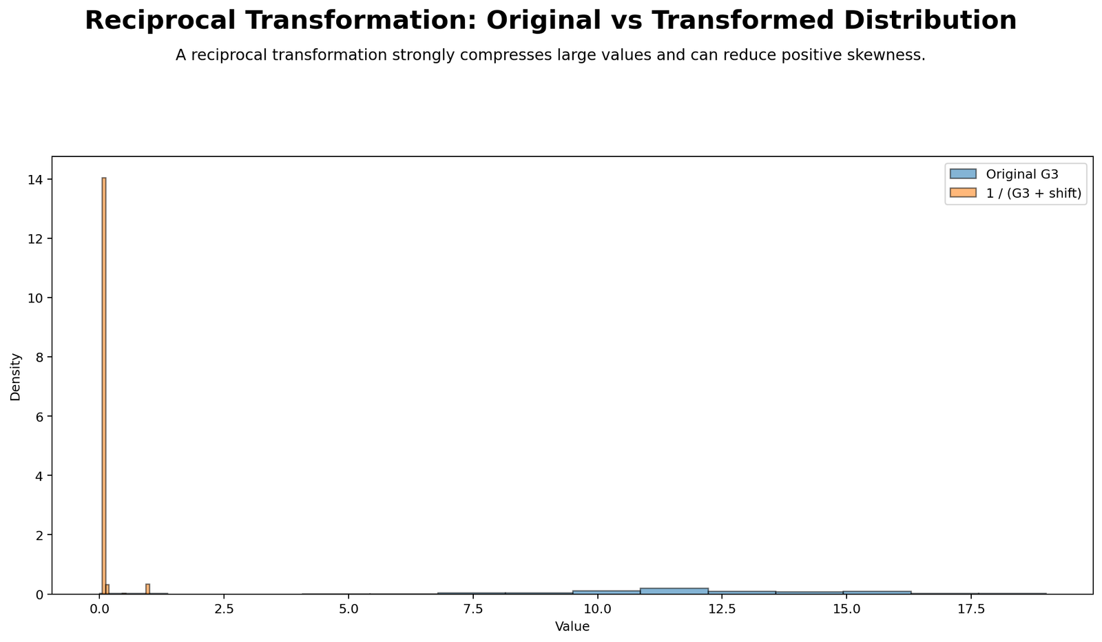
This chart shows the core effect of Reciprocal Transformation. The original distribution displays the raw scale and tail behavior, while the transformed distribution shows how the inverse formula changes the shape. High original values are compressed into small transformed values, and low original values become larger transformed values.
The interpretation depends on whether the transformed distribution is more suitable for the planned analysis. If the original variable was strongly right-skewed, the reciprocal distribution may reduce the dominance of extreme high values. However, because reciprocal transformation reverses the scale, the transformed distribution must be explained carefully in any report.
Python Chart 2: Q-Q Before and After Reciprocal Transformation
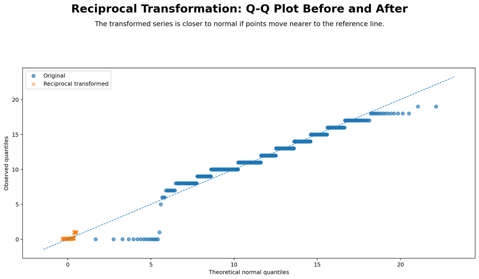
This chart compares Q-Q plots before and after Reciprocal Transformation. The original Q-Q plot shows how the raw data depart from the expected normal line. The transformed Q-Q plot shows whether the reciprocal version moves the points closer to the reference line.
If the after-transformation points are closer to the line, the transformation improved normality. If the after-transformation plot still shows strong curvature or creates a new opposite-tail problem, the transformation may not be the best choice. The Q-Q plot is one of the most important charts for deciding whether a transformation actually helped.
Python Chart 3: Skewness and Kurtosis Before and After
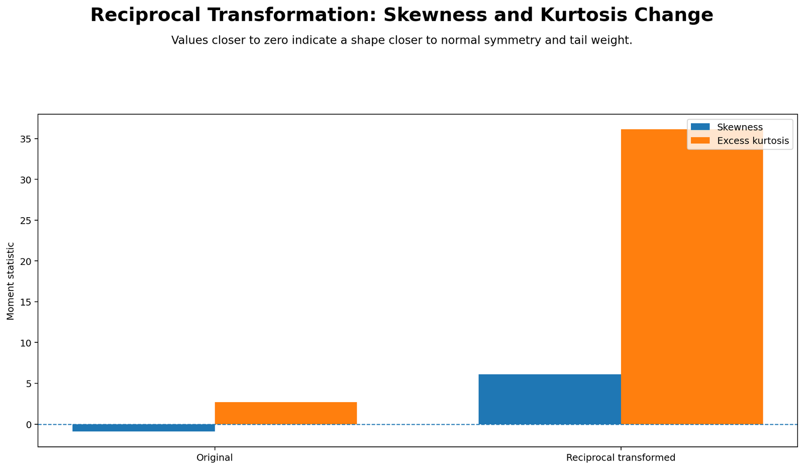
This chart summarizes the numerical shape change. A successful Reciprocal Transformation should usually move skewness closer to zero when the original variable is strongly positively skewed. Kurtosis may also move closer to a more acceptable range if extreme high values caused heavy tails.
This chart is important because it connects the visual transformation to measurable statistics. If skewness and kurtosis improve after transformation, the statistical evidence supports the visual evidence. If the transformation reduces one problem but creates another, the report should state that the transformation was only partially successful.
Python Chart 4: Normality P-values Before and After
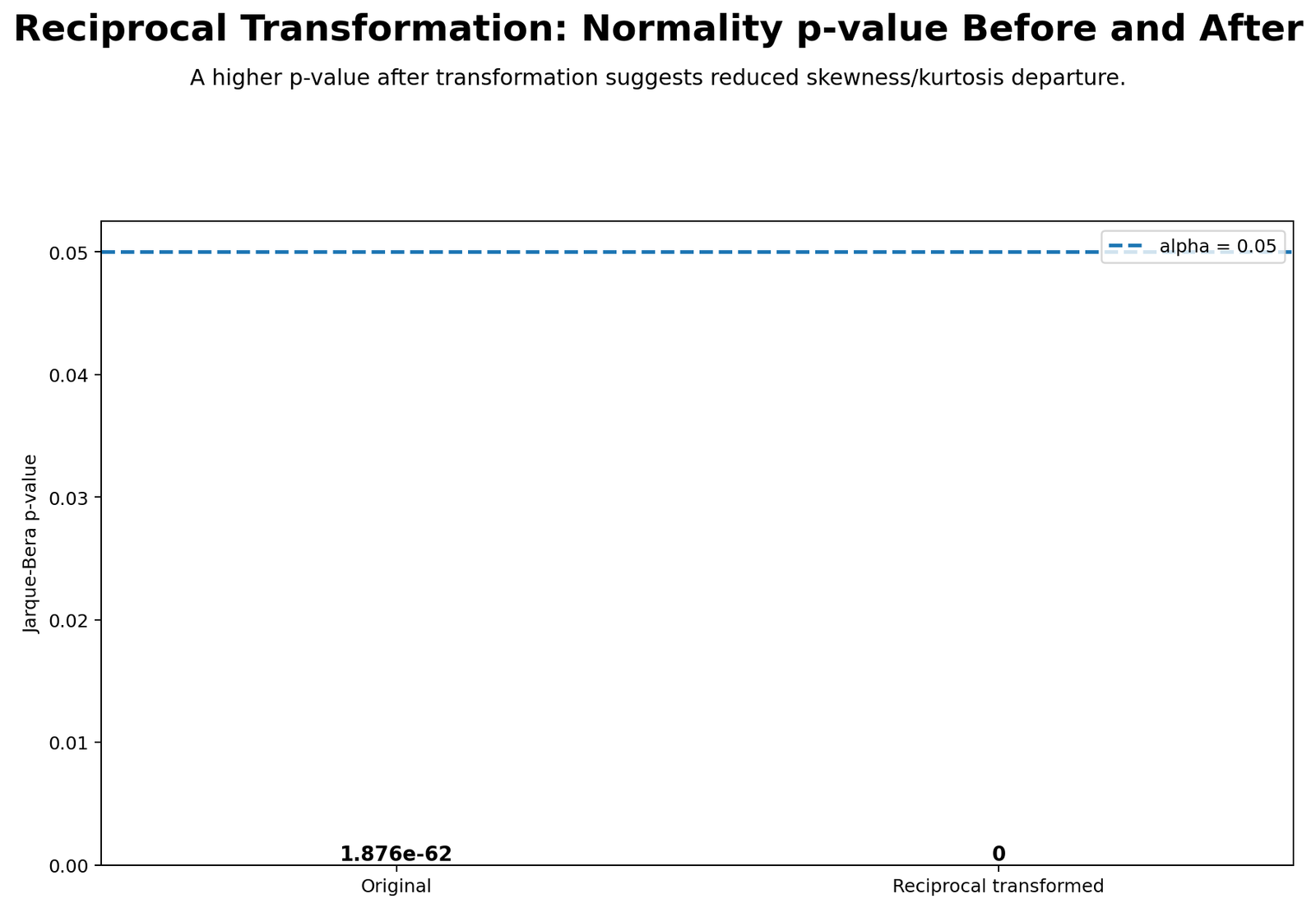
This chart shows whether formal normality-test p-values improved after Reciprocal Transformation. If the p-value increases after transformation, the transformed variable is closer to normality under that test. If the p-value remains very small, the transformation may not fully solve the normality problem.
The p-value chart should not be used alone. Normality p-values are sensitive to sample size. A large sample can reject normality even when the visual departure is moderate. Therefore, this chart should be interpreted with the Q-Q plot, histogram, skewness and kurtosis.
Python Chart 5: Reciprocal Transformation Curve
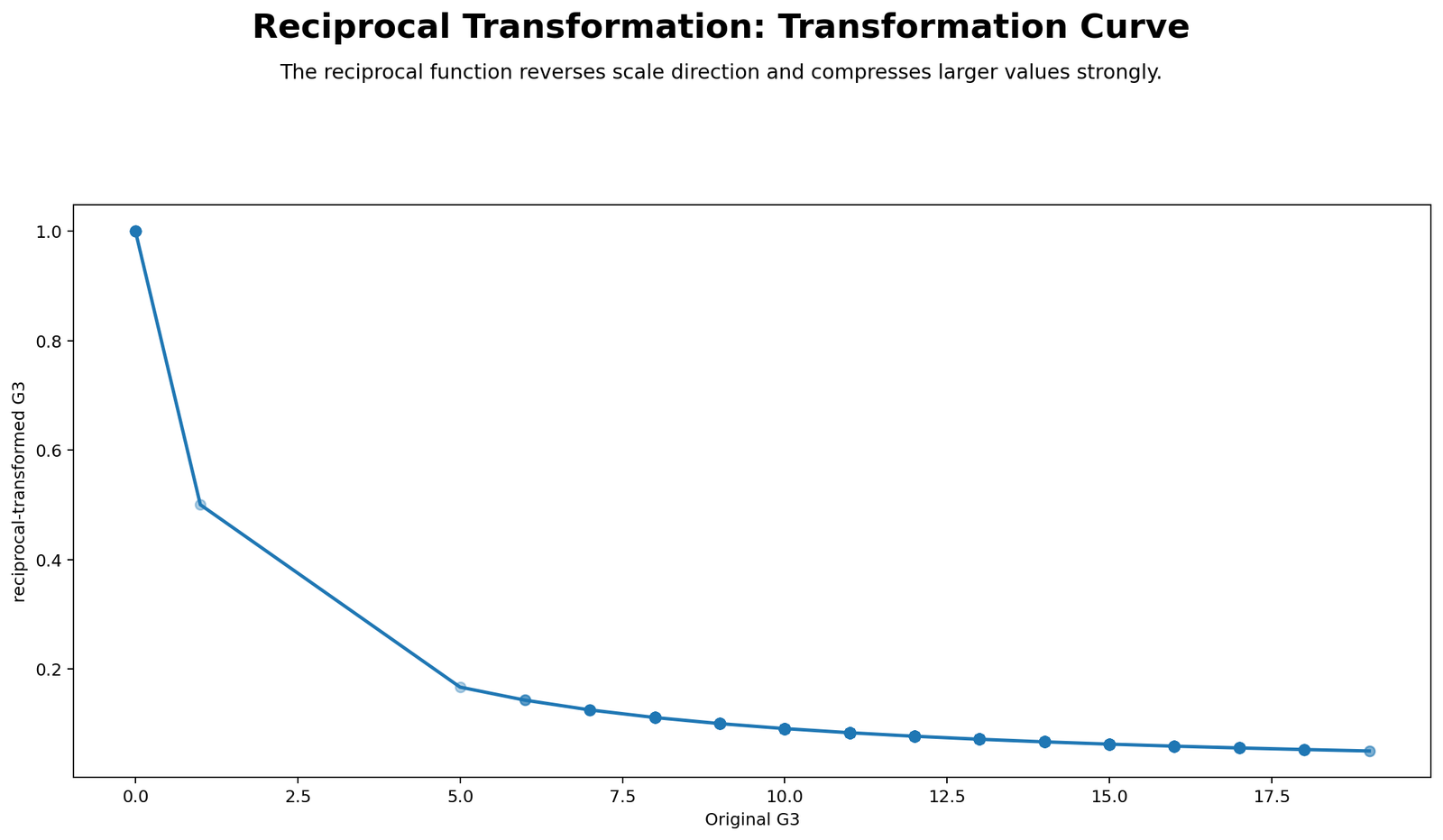
This curve explains the mathematics behind Reciprocal Transformation. As original values increase, reciprocal values decrease and move closer to zero. This is why the transformation compresses very large values. The curve also shows why interpretation changes direction: a higher original value corresponds to a lower transformed value.
The curve is useful for teaching and reporting because it makes the scale reversal clear. When using reciprocal-transformed values in a model, a positive coefficient on the transformed variable does not mean the same thing as a positive coefficient on the original variable. The transformed scale must be interpreted in inverse terms.
Python Chart 6: Group Boxplots Before and After
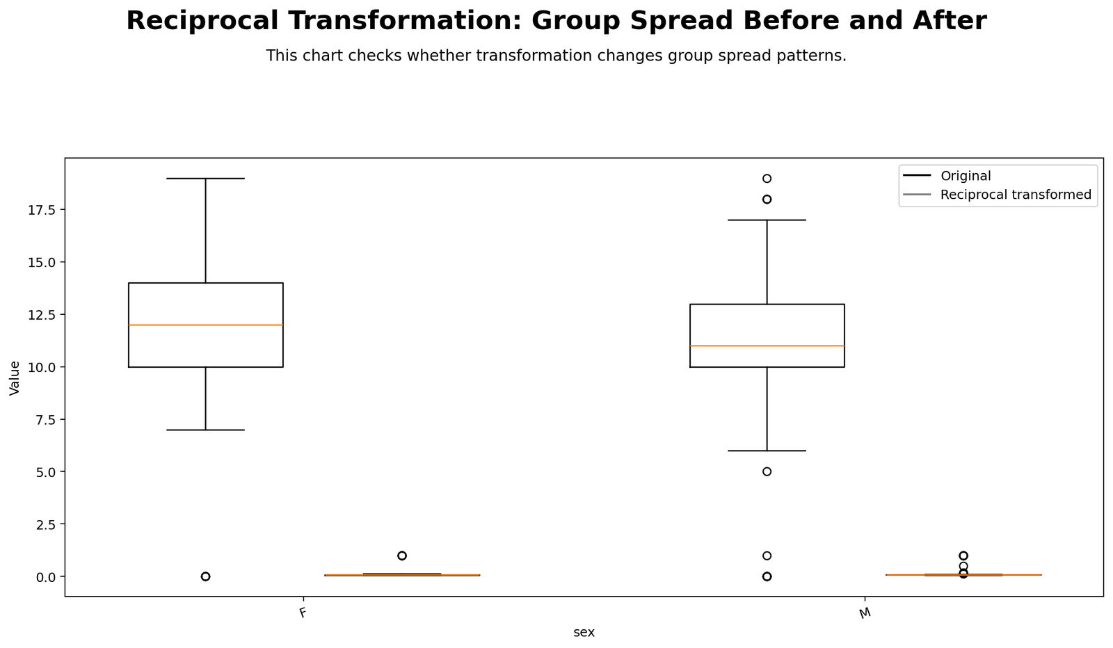
This chart compares the original and reciprocal-transformed distributions by group. Group boxplots help determine whether the transformation reduces extreme values, changes group spread, or improves comparability across groups. If the original boxplots show long upper whiskers and many high outliers, the reciprocal version may compress them.
However, group interpretation must be careful. Because the reciprocal scale is reversed, a group with larger original values may appear lower on the reciprocal scale. The chart should therefore be interpreted as a transformed-scale diagnostic, not as a direct original-scale comparison.
Python Chart 7: Skewness Across Variables
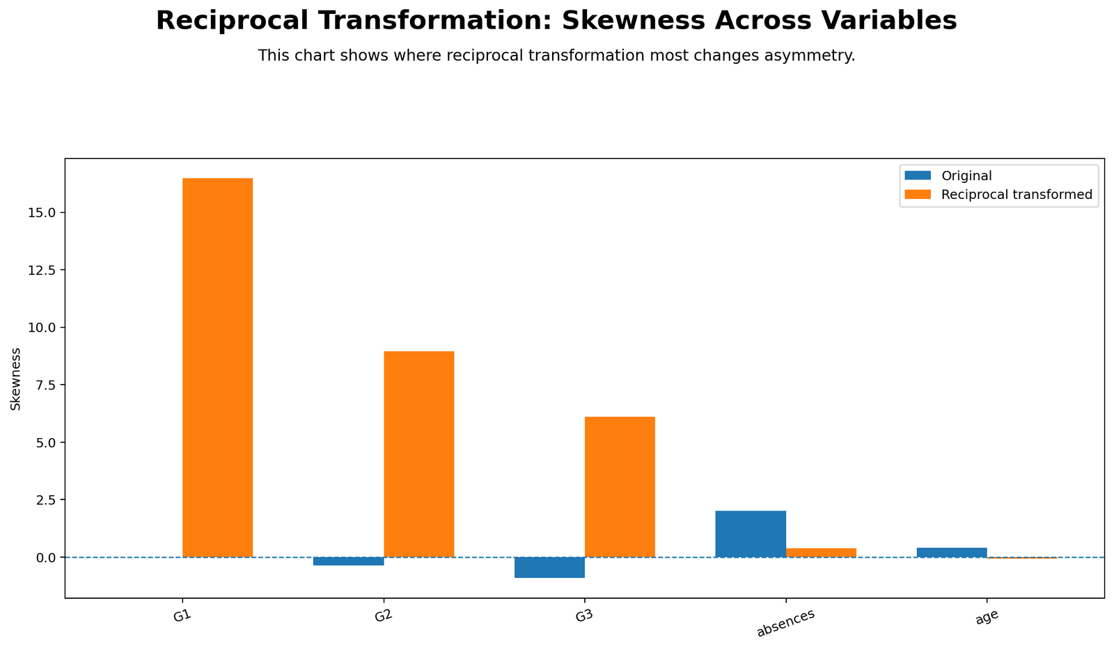
This chart shows which variables have the strongest skewness and may be candidates for transformation. Reciprocal Transformation is most relevant when a variable has strong positive skewness and high-value tail influence. Variables with near-zero skewness do not usually need reciprocal transformation.
The chart is useful because transformation should be targeted, not automatic. It helps decide whether reciprocal transformation is appropriate for one variable while leaving other variables in their original form.
R Chart-by-Chart Validation
The R charts validate the Python Reciprocal Transformation interpretation using a separate workflow. The same before-after structure appears again: distribution comparison, Q-Q plot comparison, skewness and kurtosis comparison, normality p-values, transformation curve, group boxplots and skewness across variables.
R Chart 1: Original vs Reciprocal Distribution
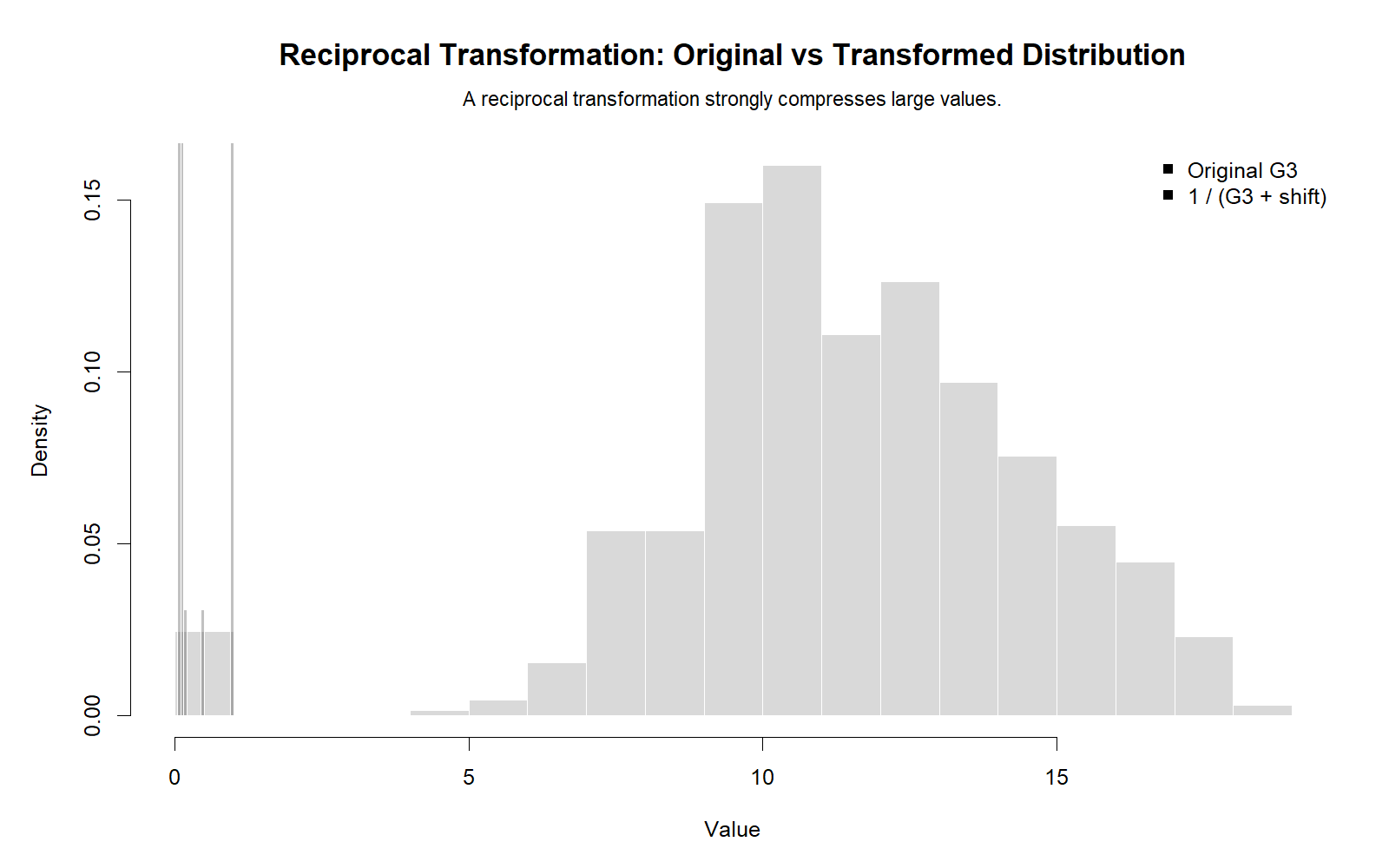
The R distribution chart confirms the Python result. The reciprocal-transformed variable changes the distribution shape by compressing large original values. This validates the core transformation effect and confirms that the result is not dependent on one software package.
R Chart 2: Q-Q Before and After Reciprocal Transformation
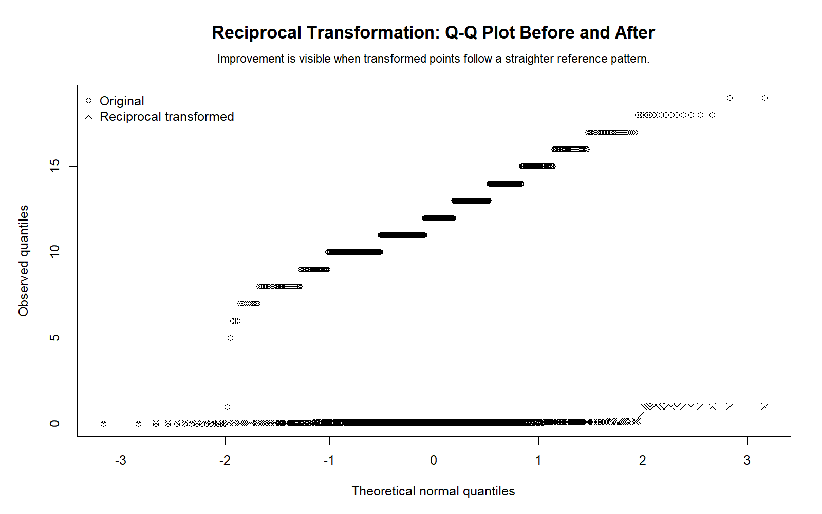
The R Q-Q comparison validates whether the transformation improved normality alignment. If the transformed points are closer to the diagonal reference line, the reciprocal transformation helped. If not, another transformation or robust method may be more appropriate.
R Chart 3: Skewness and Kurtosis Before and After
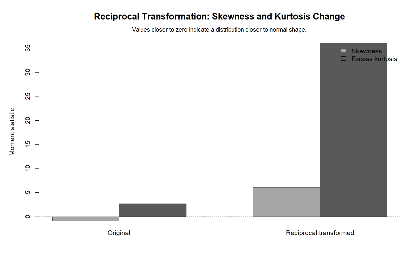
The R skewness and kurtosis chart confirms the shape-statistic comparison. A useful transformation should reduce problematic skewness and tail extremity. This chart supports the before-after decision by showing whether the transformed variable improved numerically.
R Chart 4: Normality P-values Before and After
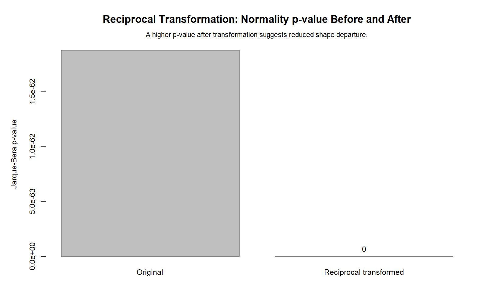
The R p-value chart validates the normality-test comparison. If the transformed p-value increases, this supports improvement. If it stays very small, the transformation did not fully resolve normality. The result should still be interpreted with Q-Q plots and histograms.
R Chart 5: Reciprocal Transformation Curve
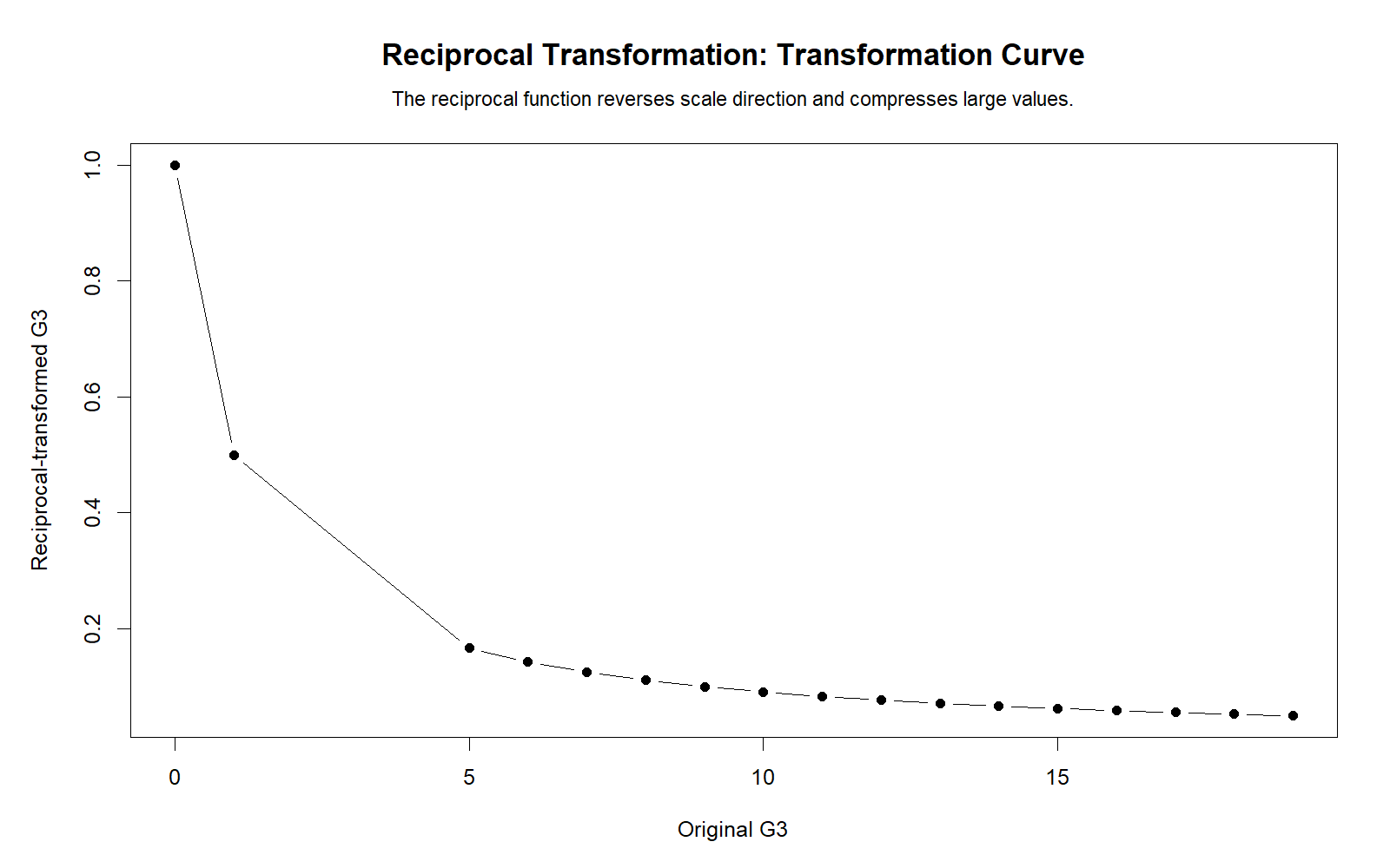
The R transformation curve confirms the same mathematical relationship shown in Python. Higher original values become lower reciprocal values. This chart is essential for explaining why interpretation reverses after transformation.
R Chart 6: Group Boxplots Before and After
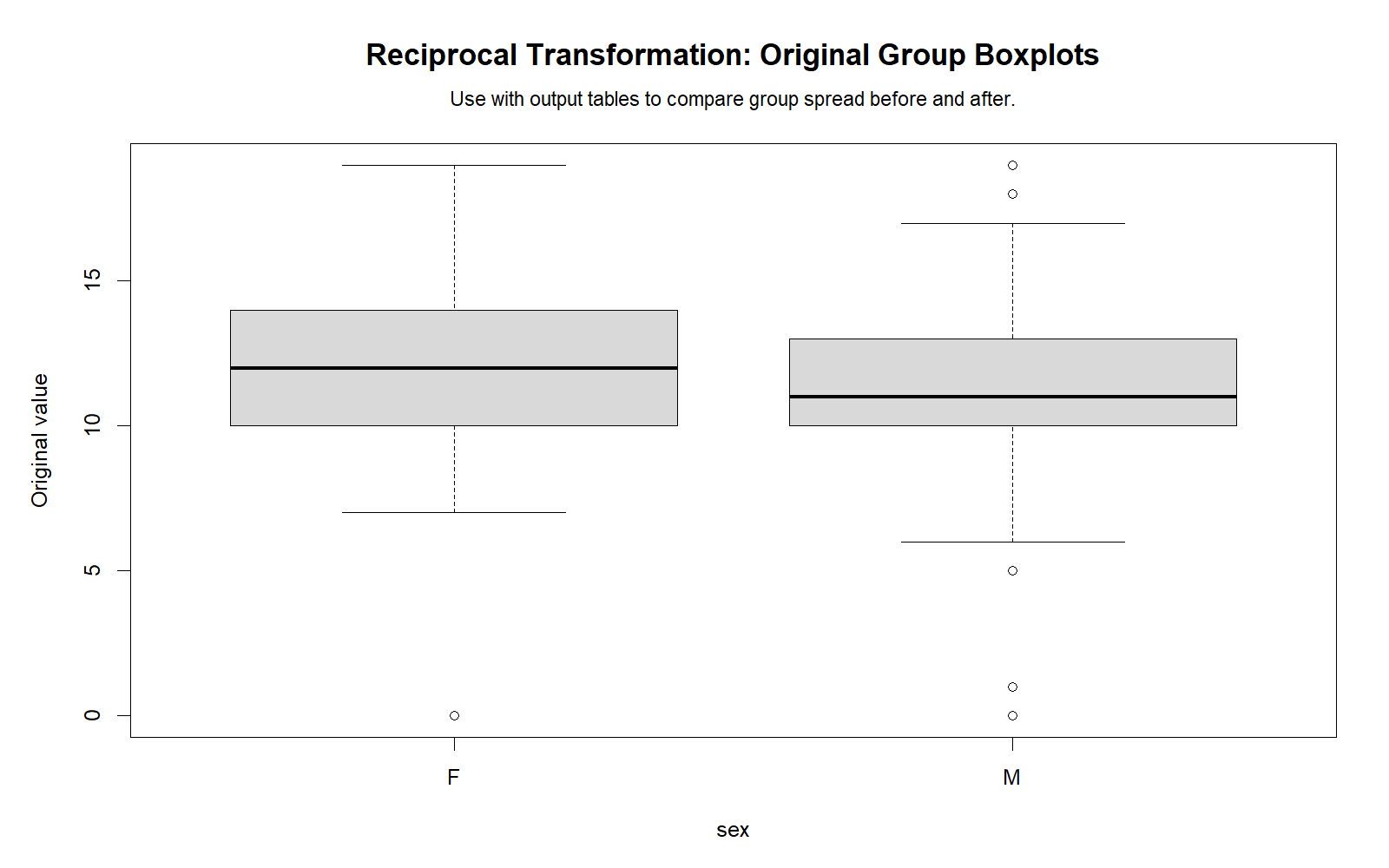
The R group boxplot chart validates the grouped transformation interpretation. It shows whether the reciprocal transformation reduces extreme high values and changes group spread. This is useful when the transformed variable will be used in group comparisons or models.
R Chart 7: Skewness Across Variables
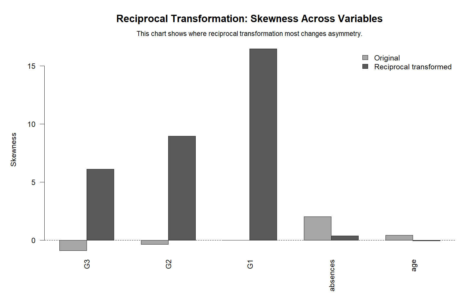
The R skewness-across-variables chart confirms that reciprocal transformation should be considered for variables with strong positive skewness rather than applied to every variable. This supports a targeted transformation workflow and avoids unnecessary changes to variables that are already reasonably symmetric.
SPSS, R, Python and Excel Workflows for Reciprocal Transformation
The same Reciprocal Transformation can be created in SPSS, R, Python and Excel. The workflow is always the same: choose a suitable positive or zero-shifted variable, compute the reciprocal version, compare the original and transformed distributions, check normality, and decide whether the transformed variable is useful and interpretable.
SPSS Workflow
| Step | SPSS Action | Purpose |
|---|---|---|
| Inspect original variable | Analyze > Descriptive Statistics > Explore | Check histogram, skewness, kurtosis and outliers. |
| Create reciprocal variable | Transform > Compute Variable | Use 1/(absences+1) when zeros are present. |
| Compare distributions | Explore original and transformed variables | Check whether shape improves. |
| Check Q-Q plots | Normality plots with tests | Assess normality before and after transformation. |
| Compare normality p-values | Tests of normality table | Determine whether p-values improve. |
| Export PDF | OUTPUT EXPORT or File > Export | Save the verified SPSS output. |
R Workflow
| Step | R Action | Purpose |
|---|---|---|
| Read data | read.csv() | Load the dataset. |
| Create transformed variable | 1 / (x + 1) | Apply zero-safe reciprocal transformation. |
| Compare skewness | e1071::skewness() | Check shape before and after. |
| Compare kurtosis | e1071::kurtosis() | Check tail behavior before and after. |
| Create Q-Q plots | qqnorm() and qqline() | Visualize normality improvement. |
| Create charts | Base R or ggplot2 | Build before-after figures. |
Python Workflow
| Step | Python Action | Purpose |
|---|---|---|
| Read data | pandas.read_csv() | Load the dataset. |
| Select variable | df["absences"] | Choose the skewed variable. |
| Create reciprocal variable | 1 / (x + 1) | Avoid division by zero. |
| Calculate diagnostics | scipy.stats.skew, kurtosis, normality tests | Compare before and after. |
| Create Q-Q plots | scipy.stats.probplot | Check normality visually. |
| Create charts | matplotlib | Build distribution, curve, p-value and group charts. |
Excel Workflow
| Excel Task | Formula or Tool | Purpose |
|---|---|---|
| Original variable | Place values in column A | Prepare original data. |
| Create reciprocal variable | =1/(A2+1) | Use zero-safe reciprocal transformation. |
| Calculate skewness | =SKEW(range) | Compare skewness before and after. |
| Calculate kurtosis | =KURT(range) | Compare tail behavior before and after. |
| Create histogram | Insert > Statistical Chart > Histogram | Visualize distribution before and after. |
| Create Q-Q style plot | Sort values and compare with normal scores | Approximate normality plot. |
Code Blocks for Reciprocal Transformation
SPSS Syntax for Reciprocal Transformation
* Reciprocal Transformation in SPSS.
* Example variable: absences.
* Zero-safe reciprocal formula: 1 / (absences + 1).

TITLE "Reciprocal Transformation Analysis".

COMPUTE reciprocal_absences = 1 / (absences + 1).
VARIABLE LABELS reciprocal_absences "Reciprocal transformation of absences: 1/(absences+1)".
EXECUTE.

FREQUENCIES VARIABLES=absences reciprocal_absences
  /STATISTICS=MEAN MEDIAN MODE STDDEV VARIANCE SKEWNESS SESKEW KURTOSIS SEKURT RANGE MINIMUM MAXIMUM
  /HISTOGRAM NORMAL
  /ORDER=ANALYSIS.

EXAMINE VARIABLES=absences reciprocal_absences
  /PLOT BOXPLOT HISTOGRAM NPPLOT
  /COMPARE GROUPS
  /STATISTICS DESCRIPTIVES
  /CINTERVAL 95
  /MISSING LISTWISE
  /NOTOTAL.

EXAMINE VARIABLES=absences reciprocal_absences BY sex
  /PLOT BOXPLOT
  /STATISTICS DESCRIPTIVES
  /MISSING LISTWISE
  /NOTOTAL.

OUTPUT EXPORT
  /CONTENTS EXPORT=VISIBLE
  /PDF DOCUMENTFILE="Reciprocal-Transformation-SPSS-Output.pdf".
Python Code for Reciprocal Transformation
import pandas as pd
import numpy as np
from scipy import stats

df = pd.read_csv("dataset.csv")

x = pd.to_numeric(df["absences"], errors="coerce")
df["reciprocal_absences"] = 1 / (x + 1)

def describe_shape(series):
    s = series.dropna()
    return {
        "n": len(s),
        "mean": s.mean(),
        "median": s.median(),
        "sd": s.std(ddof=1),
        "skewness": stats.skew(s, bias=False),
        "kurtosis": stats.kurtosis(s, fisher=True, bias=False),
        "shapiro_p": stats.shapiro(s.sample(min(len(s), 500), random_state=123)).pvalue
    }

original_summary = describe_shape(df["absences"])
reciprocal_summary = describe_shape(df["reciprocal_absences"])

summary_table = pd.DataFrame(
    [original_summary, reciprocal_summary],
    index=["Original absences", "Reciprocal absences"]
)

print(summary_table)

# Q-Q plot values can be created using scipy.stats.probplot
original_qq = stats.probplot(df["absences"].dropna(), dist="norm")
reciprocal_qq = stats.probplot(df["reciprocal_absences"].dropna(), dist="norm")

# Group summary
group_summary = df.groupby("sex")[["absences", "reciprocal_absences"]].agg(["count", "mean", "median", "std"])
print(group_summary)
R Code for Reciprocal Transformation
# Reciprocal Transformation in R

df <- read.csv("dataset.csv")

df$absences <- as.numeric(df$absences)
df$reciprocal_absences <- 1 / (df$absences + 1)

# install.packages("e1071")
library(e1071)

shape_summary <- function(x) {
  x <- na.omit(x)
  data.frame(
    n = length(x),
    mean = mean(x),
    median = median(x),
    sd = sd(x),
    skewness = skewness(x, type = 2),
    kurtosis = kurtosis(x, type = 2)
  )
}

original_summary <- shape_summary(df$absences)
reciprocal_summary <- shape_summary(df$reciprocal_absences)

summary_table <- rbind(
  Original = original_summary,
  Reciprocal = reciprocal_summary
)

print(summary_table)

# Q-Q plots
qqnorm(df$absences, main = "Original Absences Q-Q Plot")
qqline(df$absences)

qqnorm(df$reciprocal_absences, main = "Reciprocal Absences Q-Q Plot")
qqline(df$reciprocal_absences)

# Group summaries
aggregate(absences ~ sex, data = df, summary)
aggregate(reciprocal_absences ~ sex, data = df, summary)
Excel Formula Block for Reciprocal Transformation
Assume original absences values are in cells A2:A650.

Zero-safe reciprocal transformation:
=1/(A2+1)

Copy the formula down the full column.

Original skewness:
=SKEW(A2:A650)

Reciprocal skewness:
=SKEW(B2:B650)

Original kurtosis:
=KURT(A2:A650)

Reciprocal kurtosis:
=KURT(B2:B650)

Original mean:
=AVERAGE(A2:A650)

Reciprocal mean:
=AVERAGE(B2:B650)

Original median:
=MEDIAN(A2:A650)

Reciprocal median:
=MEDIAN(B2:B650)

Chart:
Create histograms for both columns.
Create boxplots for both columns.
Compare whether the transformed variable has less problematic skewness and tail behavior.
APA Reporting Wording for Reciprocal Transformation
APA reporting for Reciprocal Transformation should describe why the transformation was used, what formula was applied, whether a constant was added, and whether the transformed variable improved the assumption checks. The report should also explain the scale reversal.
APA-Style Transformation Report
A reciprocal transformation was applied to the positively skewed variable using the formula 1/(x + 1) because the original variable contained zero values. Before-after diagnostics were reviewed using histograms, Q-Q plots, skewness, kurtosis and normality p-values. The transformed variable was interpreted cautiously because reciprocal transformation reverses the direction of the original scale.
Short APA-Style Version
The original variable showed strong right-skewness, so a zero-safe Reciprocal Transformation, 1/(x + 1), was applied. The transformed distribution was then compared with the original distribution using Q-Q plots, skewness, kurtosis and normality p-values.
Scale-Reversal Wording
Because the reciprocal transformation reverses the scale, higher original values correspond to lower transformed values. Therefore, any interpretation of the transformed variable was made on the inverse scale and not directly as the original raw variable.
Common Mistakes in Reciprocal Transformation Interpretation
| Mistake | Why It Is a Problem | Correct Practice |
|---|---|---|
| Using 1/x when zeros exist | Division by zero is undefined. | Use a shifted formula such as 1/(x+1) when appropriate. |
| Forgetting scale reversal | High original values become low transformed values. | Explain the inverse interpretation clearly. |
| Transforming every variable | Transformation should solve a specific problem. | Use skewness and charts to choose suitable variables. |
| Using p-values alone | Normality p-values are sample-size sensitive. | Use Q-Q plots, histograms, skewness and kurtosis too. |
| Ignoring interpretability | Reciprocal values may be hard for readers to understand. | Report original-scale meaning where possible. |
| Assuming transformation always improves data | It can create new skewness or distort group comparisons. | Check before-after diagnostics before using the transformed variable. |
| Transforming negative values without checking | Negative and zero values can create difficult or undefined inverse behavior. | Inspect minimum, zeros and sign before transformation. |
Do not transform blindly: A Reciprocal Transformation should be justified by the distribution shape and the analysis goal. If the transformed variable is less interpretable and does not improve diagnostics, it should not be used as the final analysis variable.
When to Use Reciprocal Transformation
Use Reciprocal Transformation when the variable has strong positive skewness, extreme high values, a right-tail problem, or an inverse-type relationship that may become more stable after transformation. Do not use it for every skewed variable. It is strongest when the data are positive or can be shifted safely.
| Use Reciprocal Transformation When | Reason | Example |
|---|---|---|
| Variable is strongly right-skewed | Reciprocal transformation compresses high values. | Absence counts with a long right tail. |
| High values dominate the distribution | Inversion reduces their numerical influence. | Extreme counts or time values. |
| Q-Q plot has upper-tail departure | The transformation may improve normality alignment. | Before-after Q-Q plot comparison. |
| Skewness and kurtosis are extreme | The transformation can reduce shape problems. | Skewness-kurtosis before-after chart. |
| Model relationship is inverse-like | The transformed variable may fit the model better. | Outcome changes quickly at low x and slowly at high x. |
If normality or assumption issues remain after Reciprocal Transformation, consider alternatives such as robust analysis, bootstrapping, nonparametric tests, or other transformations. For assumption checks, use Q-Q plot normality check, P-P plot normality check, Levene test, Brown-Forsythe test, and Goldfeld-Quandt test.
Downloads and Resources for Reciprocal Transformation
The SPSS output PDF below verifies the Reciprocal Transformation workflow used for this guide. Use it as the supporting output file for SPSS interpretation, before-after distribution comparison, normality diagnostics and reporting.
FAQs About Reciprocal Transformation
What is Reciprocal Transformation?
Reciprocal Transformation is a data transformation that replaces each value with its inverse, usually 1/x or 1/(x+c).
What is the formula for Reciprocal Transformation?
The basic formula is 1/x. If the data contain zeros, a shifted formula such as 1/(x+1) is commonly used.
When should I use Reciprocal Transformation?
Use it when a variable has strong positive skewness, extreme high values or an inverse-type relationship that may be improved by compressing large values.
Can Reciprocal Transformation handle zero values?
The basic formula 1/x cannot handle zeros. If zeros exist, use a shifted version such as 1/(x+1), but explain the shift in the report.
Does Reciprocal Transformation reverse the scale?
Yes. Larger original values become smaller transformed values. This scale reversal must be explained when interpreting results.
Does Reciprocal Transformation always improve normality?
No. It may improve strongly right-skewed data, but it can also create new distortion. Always compare before-after histograms, Q-Q plots, skewness, kurtosis and p-values.
Is Reciprocal Transformation better than log transformation?
Not always. Log transformation is often easier to interpret and may be enough for moderate right skewness. Reciprocal transformation is stronger and should be used when justified.
How do I calculate Reciprocal Transformation in SPSS?
Use Transform > Compute Variable and enter a formula such as 1/(absences+1) for a zero-safe reciprocal transformation.
How do I calculate Reciprocal Transformation in Python?
Use df["reciprocal_x"] = 1 / (df["x"] + 1) when the variable contains zeros.
How do I calculate Reciprocal Transformation in R?
Use df$reciprocal_x <- 1 / (df$x + 1) for a zero-safe reciprocal transformation.
How do I calculate Reciprocal Transformation in Excel?
If the original value is in A2, use =1/(A2+1) for a zero-safe reciprocal transformation.
Should I report original or reciprocal-transformed results?
Report why the transformation was used, the exact formula, before-after diagnostic results, and the final interpretation. Keep original-scale meaning available whenever possible.
Can Reciprocal Transformation be used for negative values?
It can be mathematically applied to nonzero negative values, but interpretation becomes difficult. Inspect the minimum value and consider shifting or using another method.
What charts should I use after Reciprocal Transformation?
Use original versus transformed histograms, Q-Q plots before and after, skewness-kurtosis comparison, normality p-values, transformation curve and group boxplots.

