
Eta Squared, Partial Eta Squared, Omega Squared, Epsilon Squared, Cohen’s f and Variance Explained
ANOVA Effect Size: Eta Squared, Partial Eta Squared, Omega Squared, Cohen’s f, SPSS, Python, R and Excel Guide
ANOVA Effect Size explains how large a group difference is, not only whether the ANOVA F test is statistically significant. In this guide, G3 final grade is compared across four studytime groups. The output shows group means, sum of squares, eta squared, partial eta squared, omega squared, epsilon squared, Cohen’s f, variance explained, boxplot distribution, SPSS output, Python charts, R validation charts, Excel workflow, APA wording, common mistakes and FAQ schema.
Quick Answer: ANOVA Effect Size Result
The worked ANOVA Effect Size example compares G3 final grade across four studytime groups. The group means rise from about 10.844 in studytime group 1 to about 12.092 in group 2, 13.227 in group 3 and 13.057 in group 4. The F distribution chart shows an observed F value of about 15.88, while the critical F value is about 2.62. This means the group mean difference is statistically significant.
The effect-size charts show that eta squared and partial eta squared are both close to 0.069, while omega squared and epsilon squared are close to 0.064. The variance explained pie chart shows that studytime explains about 6.9% of the variation in G3, while about 93.1% remains unexplained or within-group variation. Cohen’s f is about 0.27, and the interpretation summary labels the effect as a medium effect.
Final interpretation: Studytime has a statistically significant and medium-sized effect on G3 final grade. The result is not only significant; it also explains about 6.9% of the total variation in G3. This is meaningful for educational data because student grades are influenced by many factors, so a single studytime variable explaining nearly 7% of variation is practically useful.
Important reporting point: The p value tells whether the group difference is statistically detectable. The effect size tells how large the difference is. For this output, the correct interpretation is that studytime has a significant medium effect on G3, with eta squared around .069 and Cohen’s f around .27.
Table of Contents
- What Is ANOVA Effect Size?
- ANOVA Effect Size Formula
- Diagnostic Null and Alternative Hypothesis
- Dataset and ANOVA Variables Used
- Python Chart-by-Chart Interpretation
- R Chart-by-Chart Validation
- SPSS Output Interpretation
- SPSS, R, Python and Excel Workflows
- Code Blocks for ANOVA Effect Size
- APA Reporting Wording
- Common Mistakes
- When to Use ANOVA Effect Size
- Downloads and Resources
- Related Guides
- FAQs
What Is ANOVA Effect Size?
ANOVA Effect Size measures the strength of the group effect in an ANOVA model. The ANOVA p value answers whether group means differ more than expected by random error. The effect size answers how much of the outcome variation is connected to the grouping variable.
In this example, studytime is the grouping factor and G3 final grade is the dependent variable. The ANOVA F test shows that studytime groups differ, but the effect-size output explains the size of that difference. Eta squared shows that studytime explains about 6.9% of G3 variation. Cohen’s f around 0.27 places the effect in the medium range.
Effect size is important because very large datasets can produce small p values for small differences, while smaller datasets can miss effects that are practically meaningful. A complete ANOVA report should include the F statistic, p value, group means and an effect-size measure such as eta squared, partial eta squared, omega squared, epsilon squared or Cohen’s f.
Simple definition: ANOVA effect size tells how much the group variable matters. In this example, studytime explains about 6.9% of the variation in G3, and Cohen’s f indicates a medium effect.
Effect-size interpretation is closely connected to Effect Size, Statistical Power, P Value, Confidence Interval, Null and Alternative Hypothesis, Type I and Type II Error, and T Test vs ANOVA.
ANOVA Effect Size Formula
ANOVA effect sizes are usually calculated from the same sum-of-squares table used for the F test. The between-group sum of squares represents variation explained by the group factor, while the within-group sum of squares represents unexplained variation inside the groups.
Eta Squared Formula
Eta squared estimates the proportion of total variation explained by the grouping variable. In this output, eta squared is about .069, so studytime explains about 6.9% of the total variation in G3.
Partial Eta Squared Formula
For a one-way ANOVA with one factor, eta squared and partial eta squared are often the same or very close. In this output, both are around .069.
Omega Squared Formula
Omega squared is usually a less biased estimate than eta squared because it adjusts for degrees of freedom and error variance. In this output, omega squared is about .064, slightly lower than eta squared.
Epsilon Squared Formula
Epsilon squared also adjusts the explained-variance estimate downward. In this example, epsilon squared is close to omega squared, around .064.
Cohen’s f Formula
Cohen’s f converts the explained-variance estimate into a standardized ANOVA effect-size scale. With eta squared around .069, Cohen’s f is about .27, which is labeled as a medium effect in the interpretation summary chart.
| Effect Size | Approximate Value | Meaning in This Output | Reporting Use |
|---|---|---|---|
| Eta squared | ≈ .069 | Studytime explains about 6.9% of total G3 variation. | Simple explained-variance measure. |
| Partial eta squared | ≈ .069 | Similar to eta squared in this one-way model. | Common SPSS effect-size measure. |
| Omega squared | ≈ .064 | Bias-adjusted explained-variance estimate. | Good for reporting a less inflated estimate. |
| Epsilon squared | ≈ .064 | Another adjusted explained-variance estimate. | Useful as a conservative ANOVA effect size. |
| Cohen’s f | ≈ .27 | Medium standardized ANOVA effect. | Useful for power analysis and comparison. |
Diagnostic Null and Alternative Hypothesis for ANOVA Effect Size
The ANOVA F test and ANOVA effect size answer different parts of the same research question. The F test decides whether the studytime group means differ statistically. The effect size explains how much studytime matters in practical terms.
| Question | Null or Diagnostic Statement | Result in This Output | Interpretation |
|---|---|---|---|
| ANOVA significance | H0: all studytime group means are equal. | Observed F ≈ 15.88, critical F ≈ 2.62. | Reject equal means. |
| Variance explained | Studytime explains no meaningful G3 variation. | Eta squared ≈ .069. | Studytime explains about 6.9% of G3 variation. |
| Practical size | The group effect is trivial. | Cohen’s f ≈ .27. | The effect is interpreted as medium. |
| Error variation | Most variation is not explained by the factor. | Unexplained/error ≈ 93.1%. | Other student, school and performance factors still explain most variation. |
Decision for this example: The studytime effect is statistically significant and medium in size. The result should not be described as huge because most variation remains within groups, but it should not be dismissed as trivial because studytime explains a visible and meaningful part of G3 performance.
Dataset and ANOVA Variables Used
The worked example uses the student performance dataset. The dependent variable is G3 final grade, and the grouping factor is studytime. The analysis compares mean G3 across four studytime groups and then calculates effect-size measures to show how much of the grade variation is explained by studytime.
| Variable or Output | Role | Why It Matters for ANOVA Effect Size | Where It Appears |
|---|---|---|---|
| G3 | Dependent variable | Final grade outcome being compared. | Group means, boxplot, F test and effect size. |
| studytime | Grouping factor | Explains part of the variation in G3. | Group means and explained-variance chart. |
| SS between | Explained variation | Variation attributed to studytime group differences. | Sum of squares decomposition. |
| SS within | Error variation | Variation left inside the studytime groups. | Sum of squares and pie chart. |
| F statistic | Significance test | Tests whether group means differ statistically. | F distribution chart. |
| Eta squared / omega squared / Cohen’s f | Effect size | Shows practical magnitude of the group effect. | Effect size comparison and interpretation summary. |
Before interpreting effect size, it is useful to understand Descriptive Statistics, Mean Median and Mode, Standard Deviation, Variance, Standard Error, Box Plot Interpretation, Confidence Interval, and Central Limit Theorem.
Python Chart-by-Chart Interpretation
The Python charts below show the first ANOVA effect-size workflow. They explain the group mean pattern, sum-of-squares decomposition, effect-size comparison, F statistic, variance explained, group distribution and final interpretation summary.
Python Chart 1: Group Means with 95% Confidence Intervals
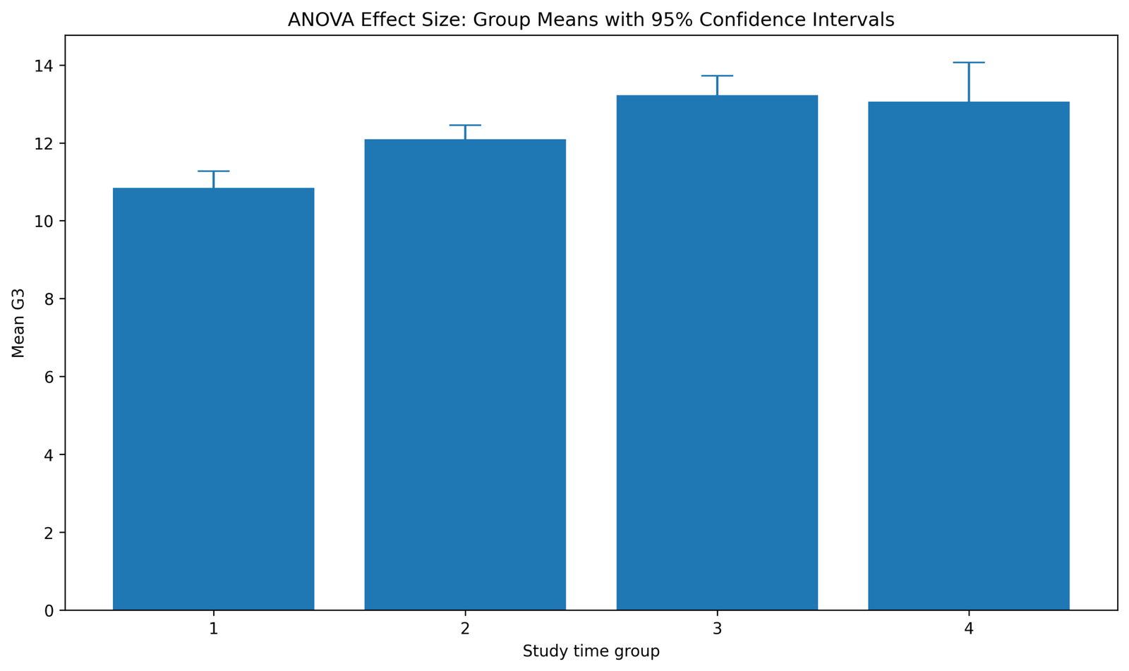
This chart shows the mean G3 score for each studytime group. Studytime group 1 has the lowest mean, group 2 is higher, group 3 has the highest mean and group 4 remains close to group 3. The pattern shows a clear rise in final grade as studytime increases from the lowest category to the higher categories.
The confidence intervals show the uncertainty around each group mean. Groups 1, 2 and 3 have comparatively tighter intervals, while group 4 has a wider interval. The wider interval for group 4 shows that its mean is less precisely estimated than the larger groups.
For ANOVA effect size, this chart explains the direction of the effect before the numerical effect-size values are reported. The effect is positive in practical terms because the higher studytime groups have higher G3 means than the lowest studytime group.
Python Chart 2: Sum of Squares Decomposition
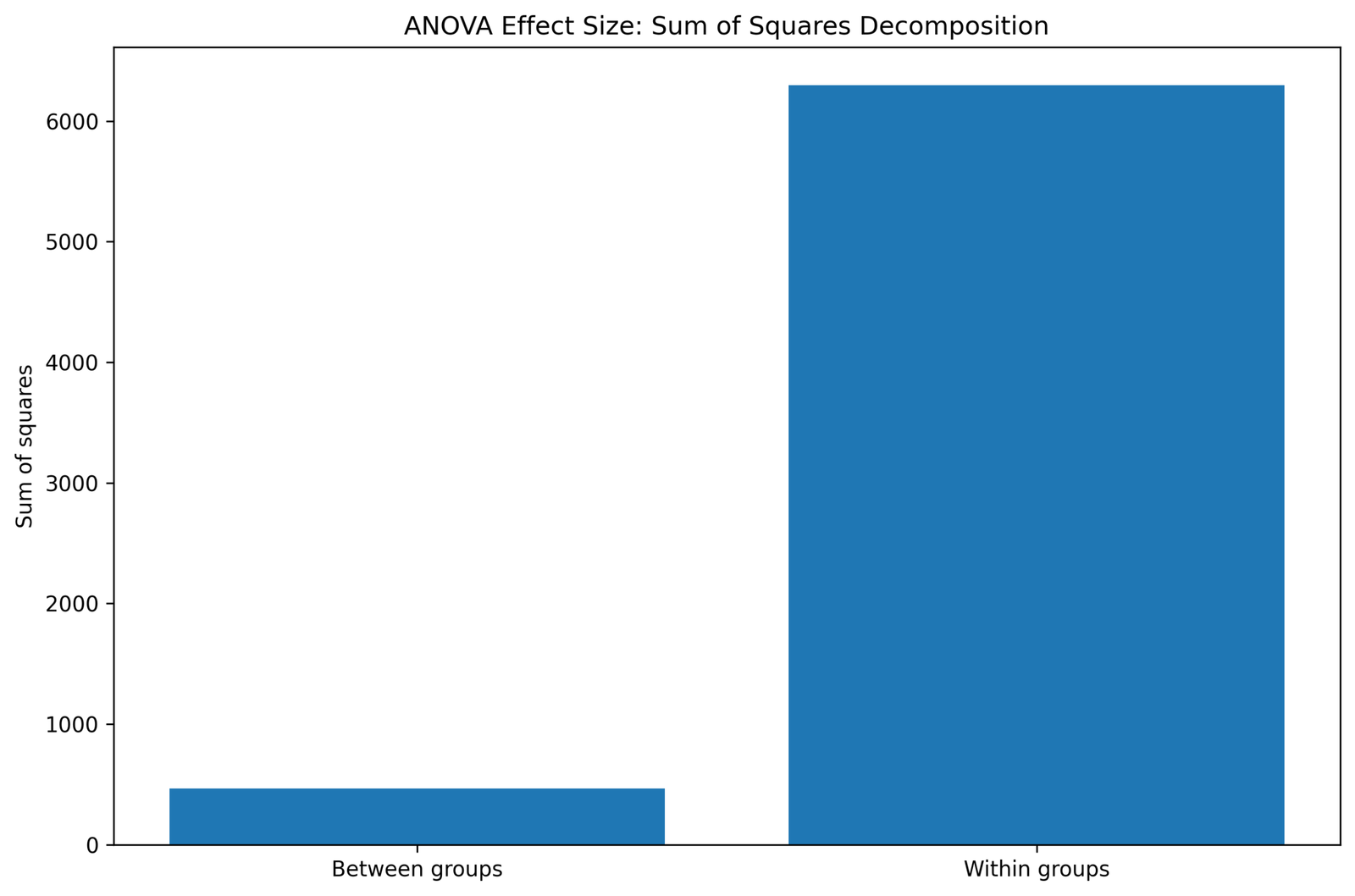
This chart separates the ANOVA variation into between-group variation and within-group variation. The between-group bar is much smaller, around 465, while the within-group bar is much larger, around 6298. This means most variation in G3 remains inside the studytime groups rather than being explained by studytime alone.
The chart does not mean studytime is unimportant. It means that student performance is influenced by many factors, so a single grouping variable explains only part of the total variation. The between-group sum of squares is still large enough relative to the error term to produce a significant F statistic.
In reporting, this chart supports the effect-size calculation. Eta squared is calculated by dividing the between-group sum of squares by the total sum of squares, which gives an explained-variance value near 6.9%.
Python Chart 3: Effect Size Comparison
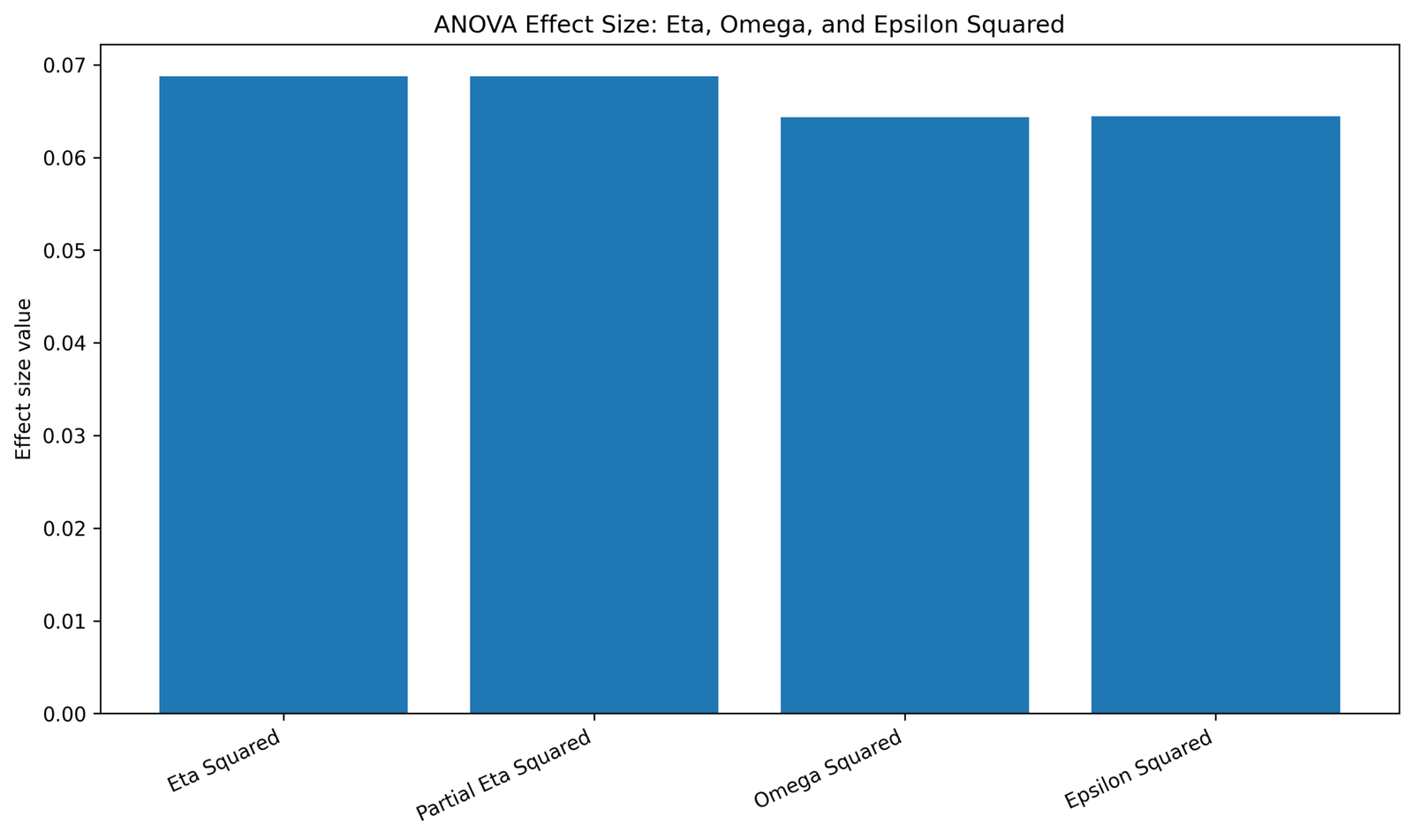
This chart compares four ANOVA effect-size estimates. Eta squared and partial eta squared are both close to .069. Omega squared and epsilon squared are slightly lower, near .064, because they adjust the explained-variance estimate downward.
The closeness of the four bars shows that the conclusion is stable across common ANOVA effect-size measures. The result is not dependent on only one formula. Whether eta squared, partial eta squared, omega squared or epsilon squared is used, the effect remains in the same practical range.
In reporting, eta squared is easiest for readers because it directly means about 6.9% explained variance. Omega squared or epsilon squared can be added as less biased estimates, especially when the article wants a more conservative effect-size statement.
Python Chart 4: F Statistic Distribution Curve
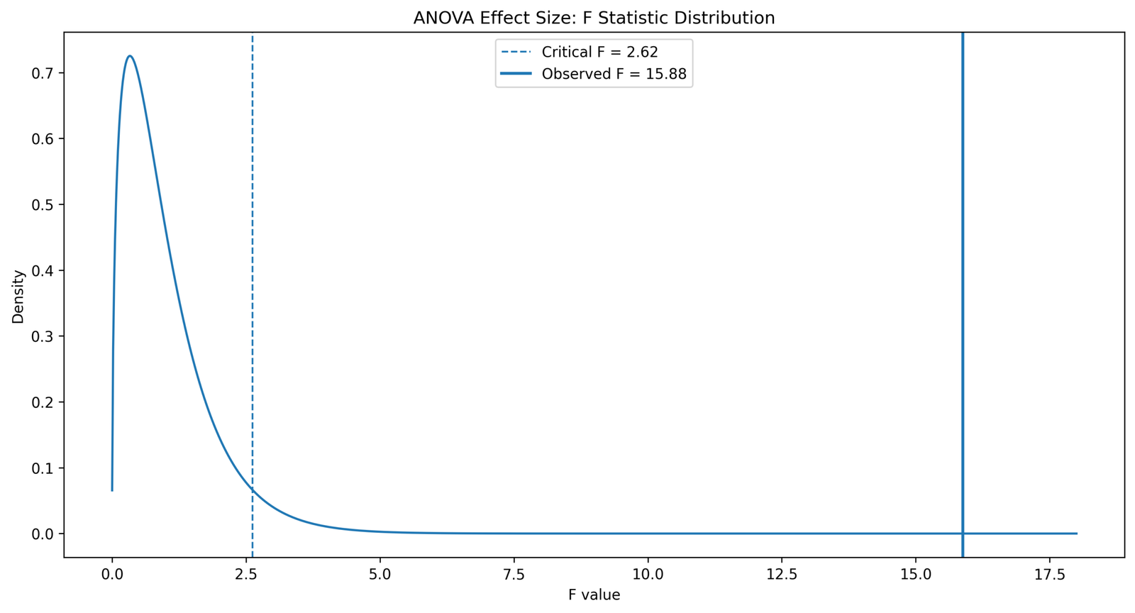
This chart shows the ANOVA F distribution with a critical F value of about 2.62 and an observed F value of about 15.88. The observed F statistic is far to the right of the critical value.
The chart shows that the group mean differences are statistically significant. The observed F value is not close to the rejection boundary; it is far beyond it, which supports a very small p value.
In reporting, this chart should be used to connect significance with effect size. The result can be written as statistically significant, but the practical interpretation should then use eta squared, omega squared and Cohen’s f rather than stopping at the F test.
Python Chart 5: Variance Explained Pie Chart
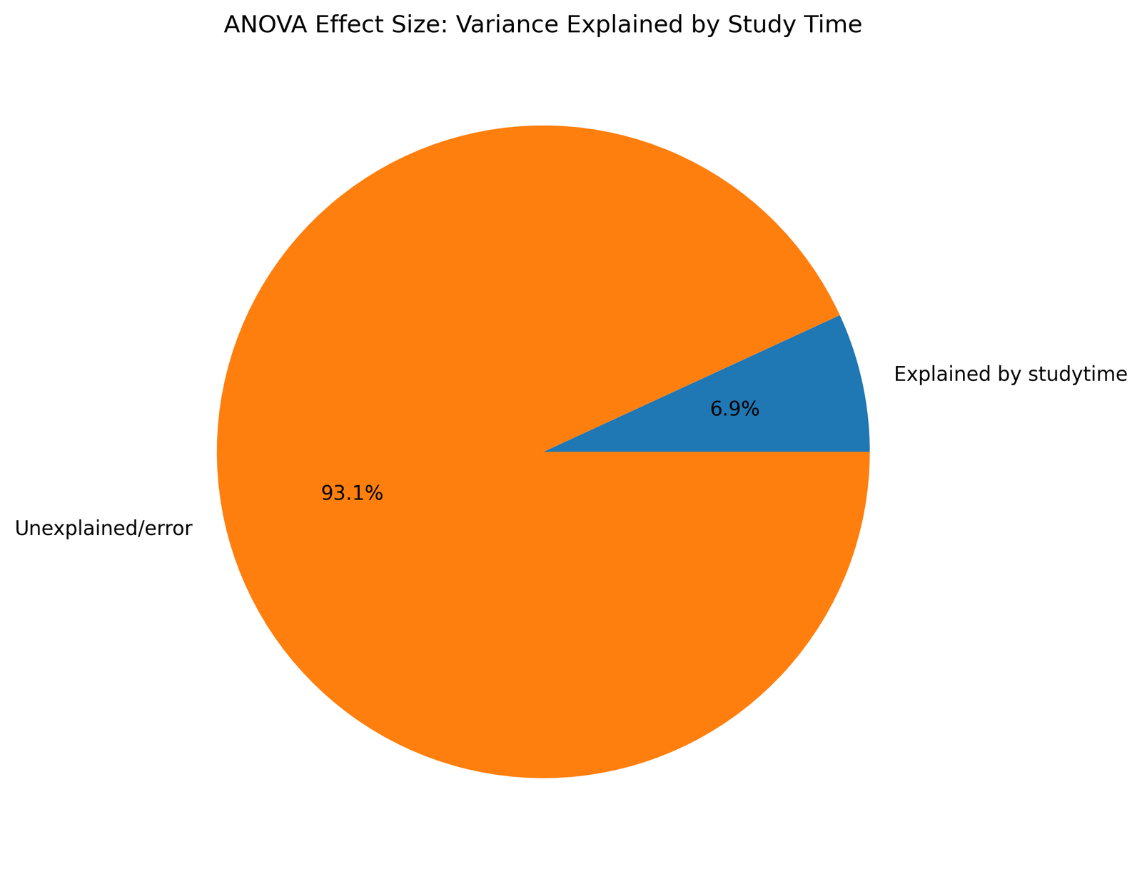
This pie chart shows the practical meaning of eta squared. Studytime explains about 6.9% of the variation in G3, while about 93.1% remains unexplained or inside the groups.
The result is realistic for educational data. Final grades are affected by previous grades, attendance, failures, school context, study habits, family background and many other variables. Studytime explains a visible part of G3, but it is not the only factor.
In reporting, this chart supports the phrase “studytime explained approximately 6.9% of the variance in G3.” This is clearer for students than only reporting eta squared = .069.
Python Chart 6: G3 Distribution by Studytime Group
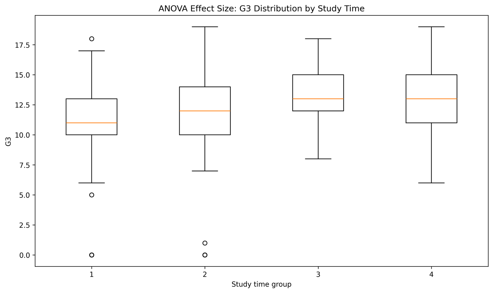
This boxplot shows the distribution of G3 scores across the four studytime groups. The median rises from studytime group 1 to groups 3 and 4. Group 1 has a lower center, group 2 is slightly higher, and groups 3 and 4 are centered near the higher G3 range.
The chart also shows low outliers in groups 1 and 2. Group 1 includes very low scores, including a point near zero, and group 2 also contains low values near zero and one. Groups 3 and 4 have higher centers and do not show the same low-outlier pattern in this figure.
For ANOVA effect-size interpretation, the boxplot explains why the effect is medium rather than tiny. The group distributions overlap, so studytime does not completely separate G3 scores, but the centers are clearly higher in the higher studytime groups.
Python Chart 7: Effect Size Interpretation Summary
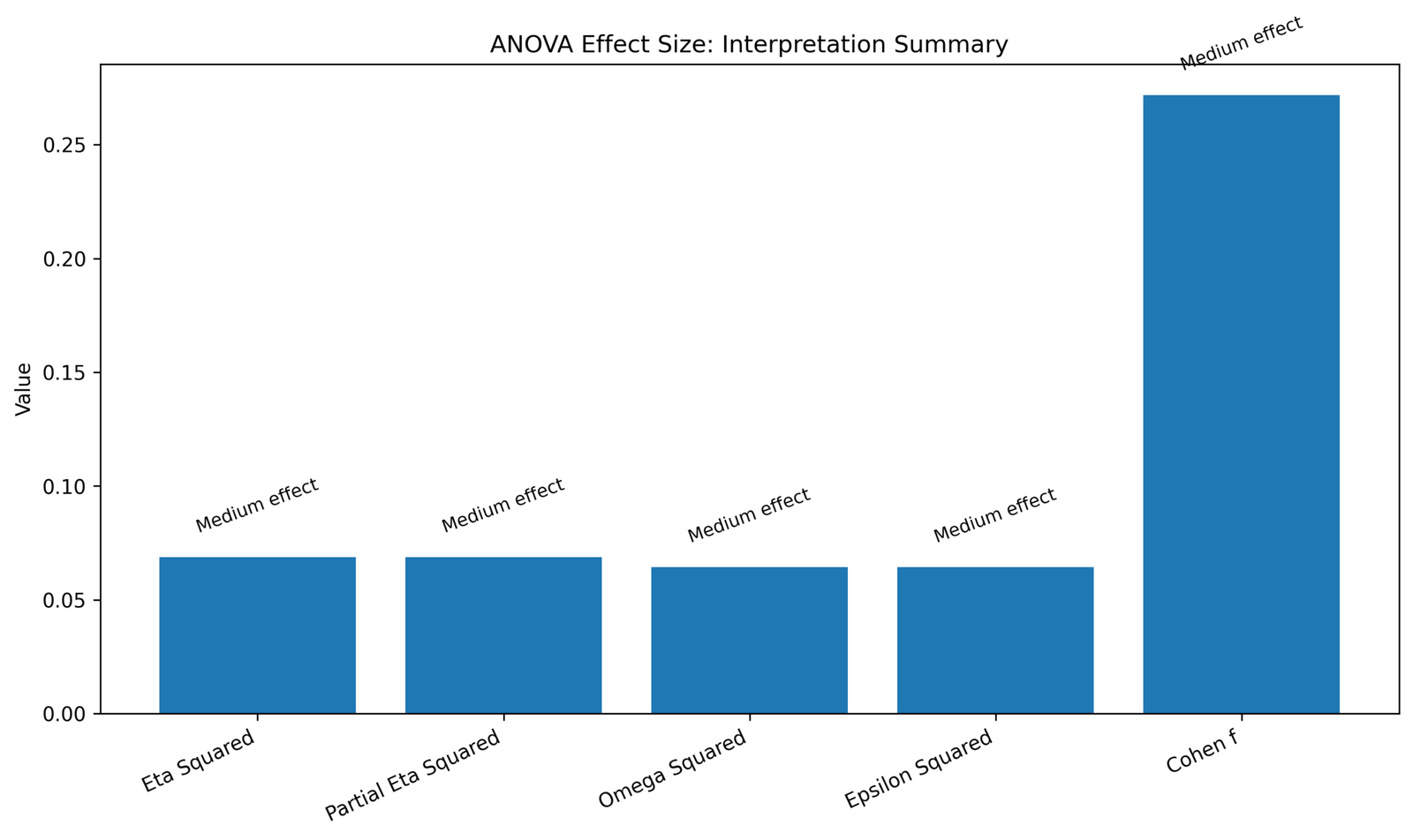
This summary chart places eta squared, partial eta squared, omega squared, epsilon squared and Cohen’s f together. The explained-variance measures sit around .064 to .069, while Cohen’s f is around .27.
The chart labels the effect as a medium effect. This is the most useful plain-language interpretation for readers because it connects the numeric effect-size values with a practical category.
In the final report, this chart supports the sentence: “The studytime effect was statistically significant and medium in size, with η² around .069 and Cohen’s f around .27.” This gives both statistical and practical meaning.
R Chart-by-Chart Validation
The R validation charts repeat the same ANOVA effect-size workflow in a second software environment. The R outputs confirm the same group mean pattern, sum-of-squares structure, effect-size range, F statistic result, explained-variance percentage and interpretation label.
R Chart 1: Group Means with 95% Confidence Intervals
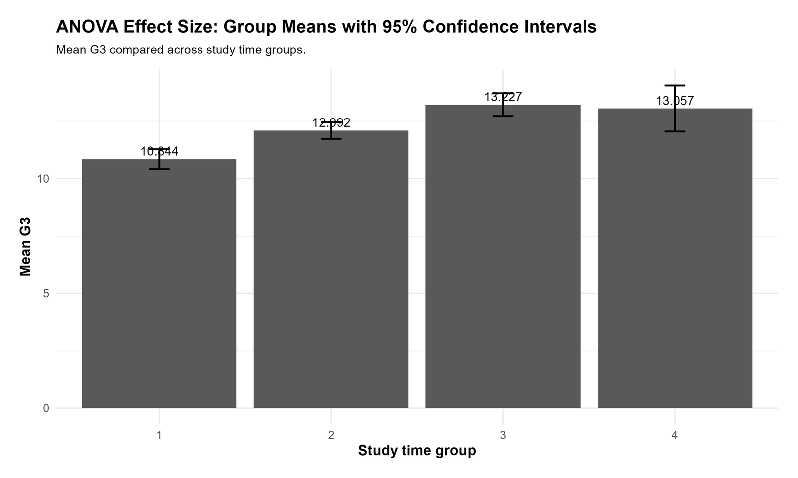
This R chart validates the same group mean pattern shown in Python. Studytime group 1 has the lowest mean G3, group 2 is higher, group 3 has the highest mean and group 4 remains close to group 3.
The confidence intervals show that the mean estimates are not equally precise across all groups. The higher uncertainty for group 4 is visible in the wider interval, while the first three groups have more compact intervals.
In reporting, this R chart confirms that the direction of the effect is stable across software. The higher studytime groups show higher final-grade performance, which gives the effect size its practical interpretation.
R Chart 2: Sum of Squares Decomposition
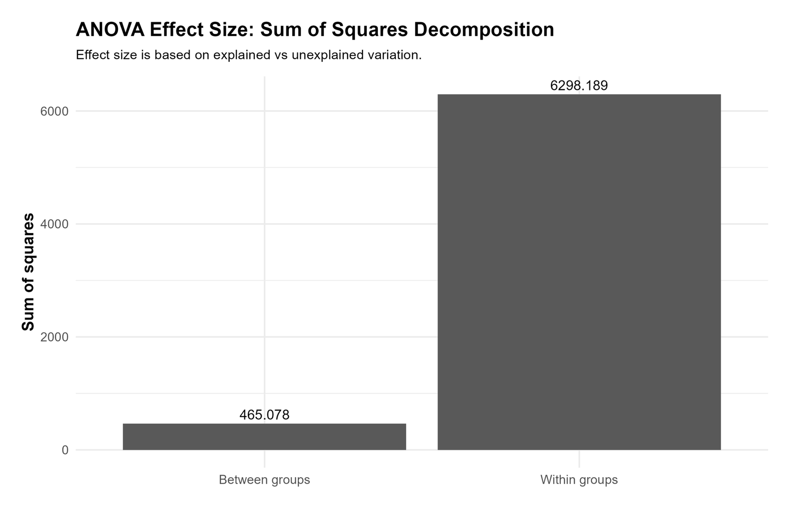
This R chart confirms that within-group variation is much larger than between-group variation. The between-group component is the part explained by studytime, while the within-group component is the error or unexplained part.
The large within-group bar explains why the pie chart shows 93.1% unexplained variation. The smaller between-group bar explains the 6.9% studytime contribution.
In reporting, this chart supports the formula behind eta squared. The effect size is not guessed from the bar chart; it is calculated from the between-group sum of squares divided by total sum of squares.
R Chart 3: Effect Size Comparison
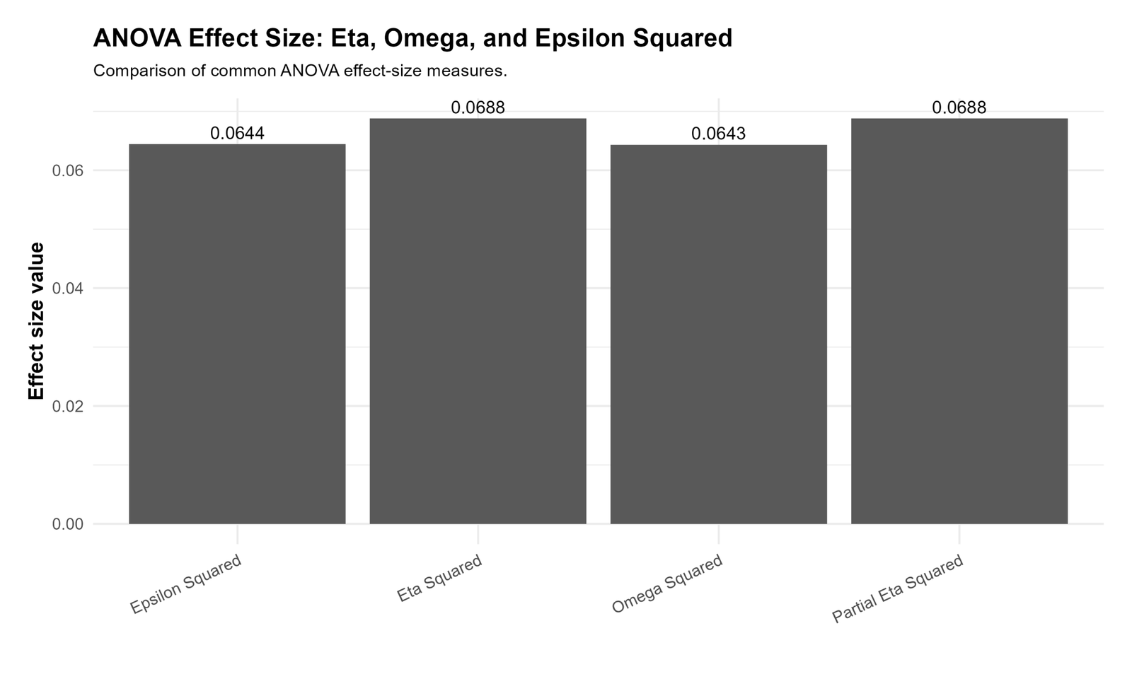
The R effect-size comparison shows the same relationship among the four estimates. Eta squared and partial eta squared are slightly higher, while omega squared and epsilon squared are slightly lower.
This pattern is expected because omega squared and epsilon squared adjust the effect-size estimate for error and degrees of freedom. They are often preferred when a less optimistic estimate is needed.
In reporting, this R chart supports a balanced conclusion: the effect is medium, and the less biased estimates still remain close to the eta squared result. The practical interpretation does not change across the measures.
R Chart 4: F Statistic Distribution Curve
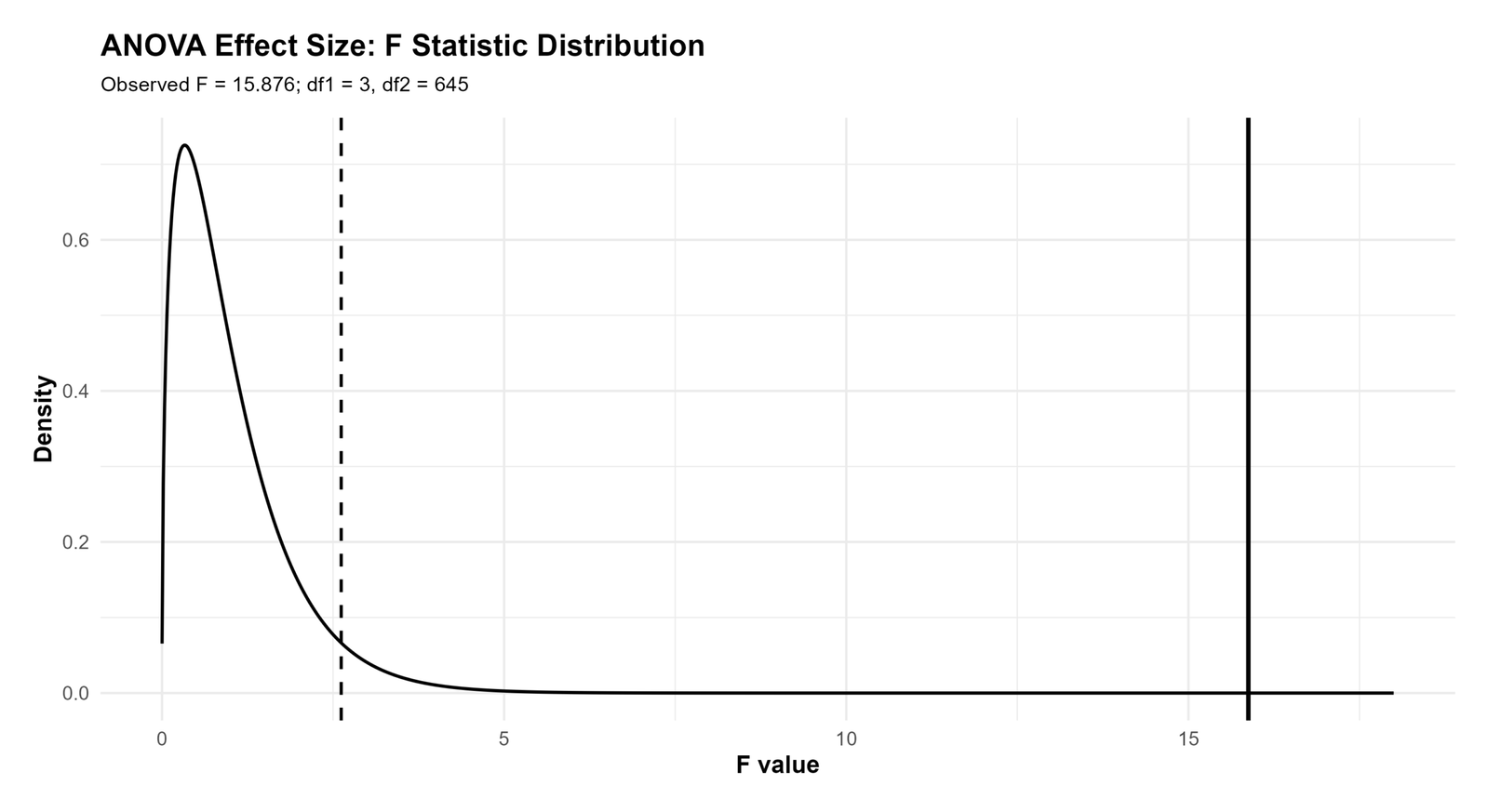
The R F distribution curve confirms the same significance decision. The observed F statistic is around 15.88, while the critical F value is around 2.62.
The observed value is far to the right of the critical value, so the studytime effect is statistically significant. This supports the statement that the group mean differences are not explained by random within-group variation alone.
In reporting, this figure should be paired with the effect-size table. The F statistic tells that the effect exists statistically, while eta squared and Cohen’s f explain how large the effect is.
R Chart 5: Variance Explained Pie Chart
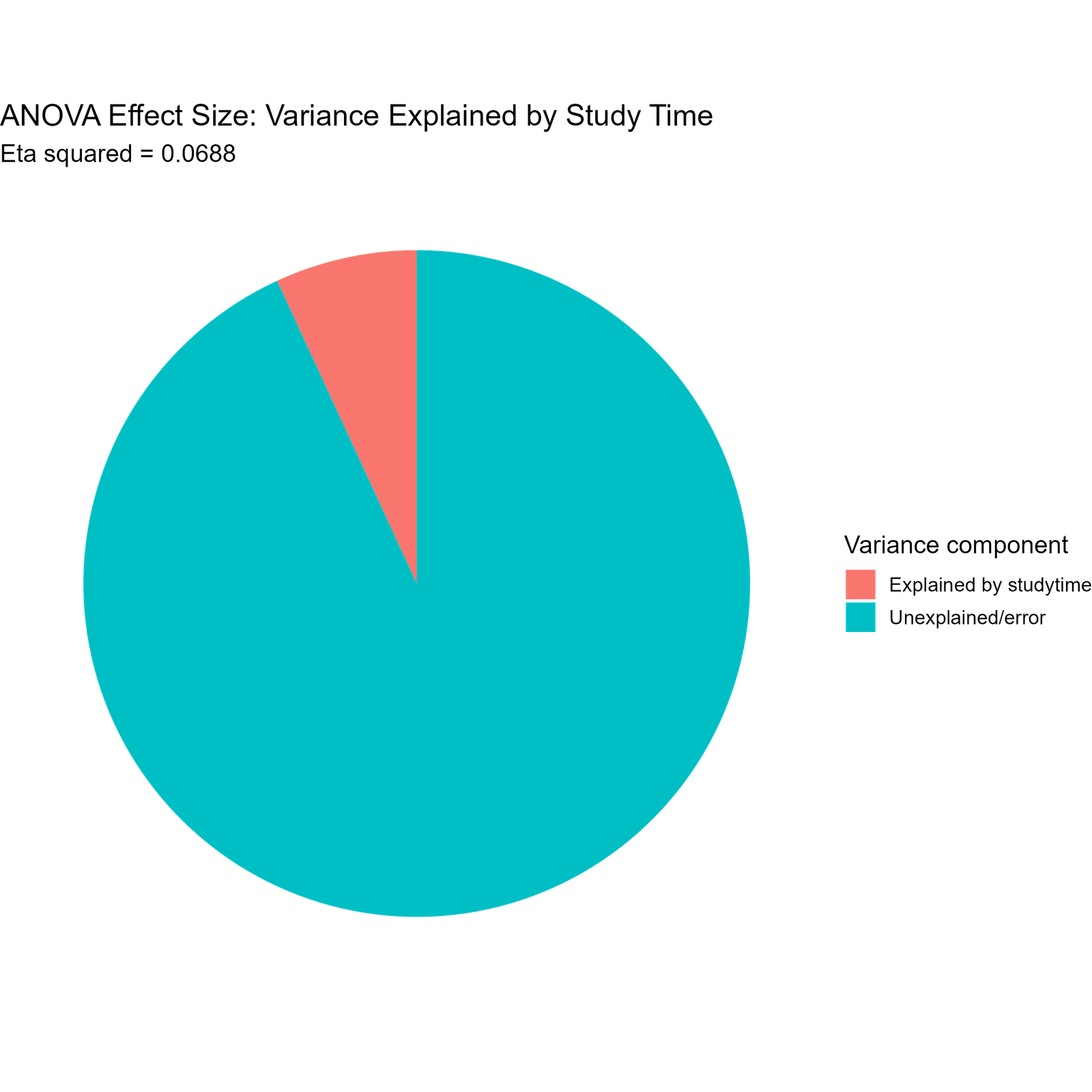
The R pie chart confirms that studytime explains about 6.9% of the variation in G3, while the remaining 93.1% is unexplained or within-group variation.
This chart is useful because it converts eta squared into a visual proportion. The effect is visible, but the large unexplained portion reminds readers that studytime is only one factor in student achievement.
In reporting, this chart supports wording such as “studytime accounted for approximately 6.9% of the variance in final grade.” That sentence is more meaningful than presenting eta squared without explanation.
R Chart 6: G3 Distribution by Studytime Group
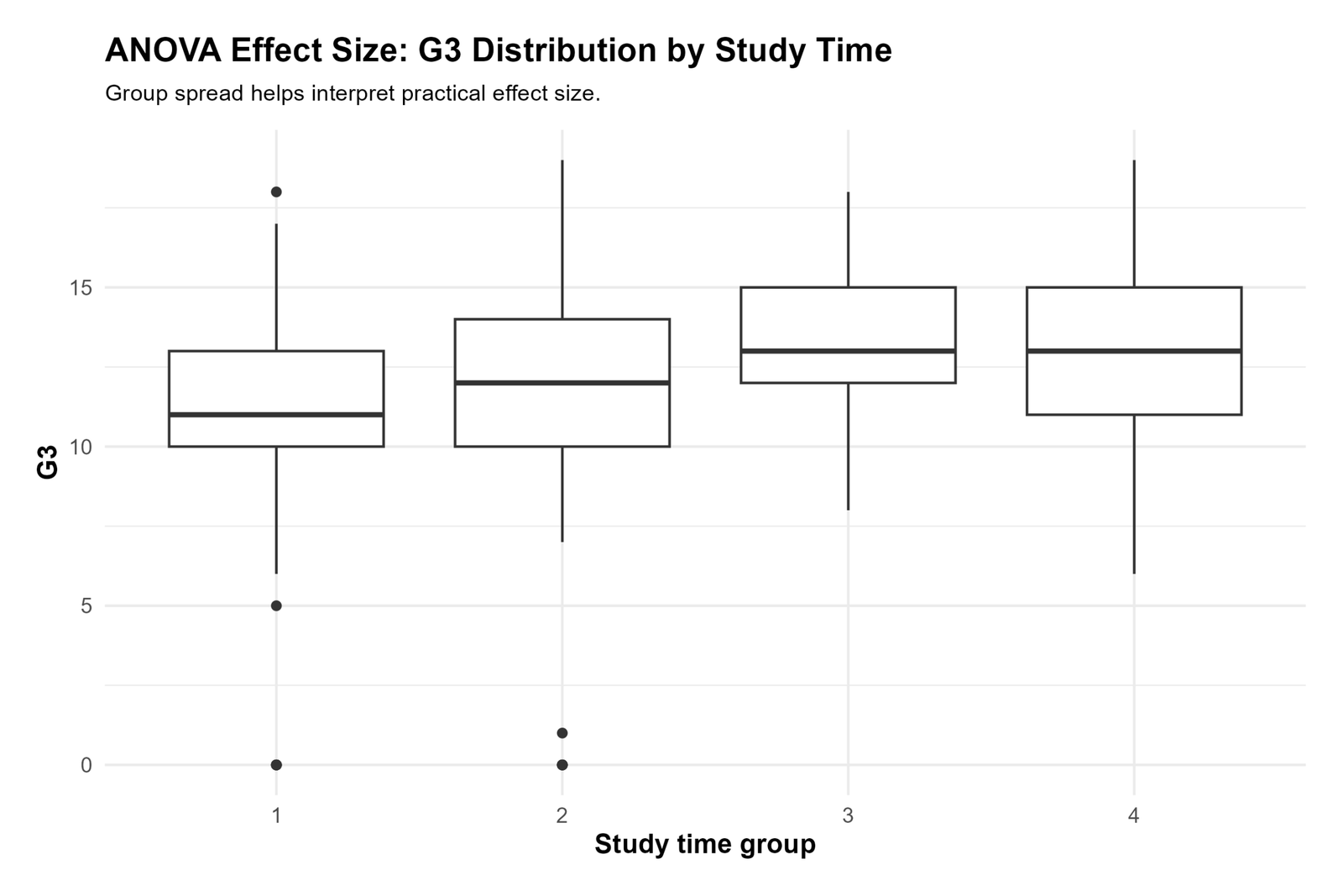
The R boxplot confirms that the higher studytime groups have higher centers than the lower studytime groups. Groups 3 and 4 are centered around higher G3 values than group 1.
The chart also confirms that the group distributions overlap. This overlap explains why the effect is medium rather than very large. Studytime helps explain G3, but it does not completely determine student performance.
In reporting, this chart should be used to connect effect size with the real distribution of scores. The group centers differ, but individual students still vary widely within each studytime group.
R Chart 7: Effect Size Interpretation Summary
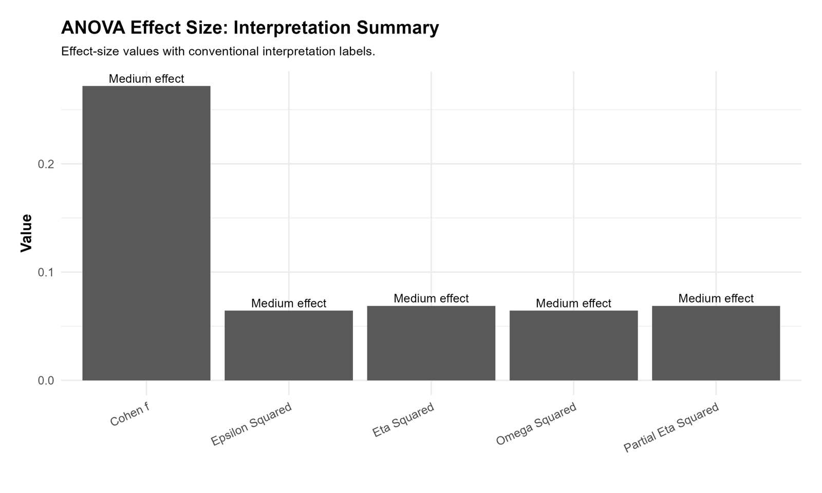
The R interpretation summary confirms the same medium-effect conclusion. The explained-variance measures remain near .064 to .069, and Cohen’s f remains near .27.
The result is consistent with the Python output. Both workflows support the same practical conclusion: studytime has a statistically significant and medium-sized association with G3 final grade.
In reporting, this chart supports the final summary sentence for the whole post: “The ANOVA effect size indicated a medium studytime effect on G3, with approximately 6.9% of variance explained.”
SPSS Output Interpretation for ANOVA Effect Size
The SPSS output PDF should be used as the final software verification file for the ANOVA Effect Size workflow. It should contain the group descriptive output, ANOVA table, effect-size statistics, variance-explained interpretation and exported evidence used for reporting.
Download ANOVA Effect Size SPSS Output PDF
SPSS Output Items to Read
| SPSS Output Item | What It Shows | How It Is Used | Reporting Meaning |
|---|---|---|---|
| Descriptives | Group n, mean, standard deviation and confidence interval. | Shows which studytime groups have higher G3 means. | Report the group means before the effect-size interpretation. |
| ANOVA table | Between-group and within-group sum of squares, df, mean squares, F and p. | Tests whether the group mean difference is statistically significant. | Report F, df and p value. |
| Eta squared | Explained variance from studytime. | Shows the simple proportion of variance explained. | Report as η² ≈ .069. |
| Partial eta squared | Effect variance relative to effect plus error variance. | Common effect-size measure in SPSS GLM output. | Report when SPSS provides partial η². |
| Omega squared | Bias-adjusted effect size. | Gives a more conservative estimate than eta squared. | Use when reporting a less inflated estimate. |
| Cohen’s f | Standardized ANOVA effect size. | Useful for power analysis and medium-effect interpretation. | Report as f ≈ .27 when relevant. |
SPSS PDF: Final Verification
The ANOVA Effect Size SPSS Output PDF should be placed in the downloads section and referenced inside the SPSS interpretation section. The PDF gives readers a direct way to verify the software output behind the effect-size values.
The strongest SPSS-style conclusion is that studytime has a statistically significant medium effect on G3. The effect is meaningful but not dominant because studytime explains about 6.9% of the variance, while most variation remains within groups.
SPSS Reporting Summary
The SPSS report should describe the F test and the effect size together. A correct interpretation is that studytime group means differ significantly, and the magnitude of the difference is medium. Eta squared and partial eta squared are about .069, while omega squared and epsilon squared are slightly lower at about .064.
A clean SPSS-style sentence is: “The studytime effect was significant, F(3, 645) ≈ 15.88, p < .001, η² ≈ .069, indicating a medium effect and about 6.9% variance explained in G3.”
SPSS, R, Python and Excel Workflows for ANOVA Effect Size
The same ANOVA Effect Size workflow can be reproduced in SPSS, R, Python and Excel. The key outputs are group means, sum of squares, F statistic, p value, eta squared, partial eta squared, omega squared, epsilon squared and Cohen’s f.
SPSS Workflow
| Step | SPSS Menu or Syntax | Purpose |
|---|---|---|
| Open data | File > Open > Data | Load the dataset with G3 and studytime. |
| Run ANOVA | Analyze > Compare Means > One-Way ANOVA | Test mean differences across studytime groups. |
| Use GLM when effect size is needed | Analyze > General Linear Model > Univariate | Request partial eta squared and model effect output. |
| Request descriptive output | Options > Descriptive statistics | Report group means and confidence intervals. |
| Calculate extra effect sizes | Use syntax, spreadsheet or exported table | Calculate eta squared, omega squared and Cohen’s f. |
| Export output | OUTPUT EXPORT | Save the SPSS output PDF for verification. |
R Workflow
| Step | R Action | Purpose |
|---|---|---|
| Read data | read.csv("dataset.csv") | Load the dataset. |
| Set factor | df$studytime <- as.factor(df$studytime) | Define the grouping variable. |
| Fit ANOVA | aov(G3 ~ studytime, data=df) | Run the one-way ANOVA. |
| Get sum of squares | summary(model) | Extract between and within sum of squares. |
| Calculate effect sizes | effectsize::eta_squared() and related functions | Estimate eta squared, omega squared and epsilon squared. |
| Plot effect size | Bar chart and pie chart | Show practical interpretation visually. |
Python Workflow
| Step | Python Action | Purpose |
|---|---|---|
| Read data | pandas.read_csv() | Load the dataset. |
| Fit ANOVA model | ols("G3 ~ C(studytime)", data=df).fit() | Fit the group mean model. |
| ANOVA table | sm.stats.anova_lm(model, typ=2) | Extract sum of squares, df, F and p value. |
| Eta squared | ss_between / ss_total | Calculate explained variance. |
| Omega squared | Bias-adjusted formula | Estimate a less inflated effect size. |
| Cohen’s f | sqrt(eta_sq/(1-eta_sq)) | Convert explained variance to standardized ANOVA effect size. |
Excel Workflow
| Excel Task | Formula or Tool | Purpose |
|---|---|---|
| Run ANOVA | Data Analysis ToolPak > ANOVA: Single Factor | Get SS between, SS within, df, MS and F. |
| Total sum of squares | =SS_between + SS_within | Calculate total variation. |
| Eta squared | =SS_between / SS_total | Calculate proportion of variance explained. |
| Omega squared | =(SS_between - df_between*MS_within)/(SS_total + MS_within) | Calculate adjusted effect size. |
| Cohen’s f | =SQRT(EtaSquared/(1-EtaSquared)) | Calculate standardized ANOVA effect size. |
| Pie chart | Explained vs unexplained variance | Visualize eta squared as a percentage. |
Code Blocks for ANOVA Effect Size
SPSS Syntax for ANOVA Effect Size
* ANOVA Effect Size in SPSS.
* Dependent variable: G3.
* Grouping factor: studytime.

TITLE "ANOVA Effect Size: G3 by Studytime".

ONEWAY G3 BY studytime
  /STATISTICS DESCRIPTIVES HOMOGENEITY
  /MISSING ANALYSIS.

UNIANOVA G3 BY studytime
  /METHOD=SSTYPE(3)
  /INTERCEPT=INCLUDE
  /PRINT=DESCRIPTIVE ETASQ HOMOGENEITY
  /CRITERIA=ALPHA(.05)
  /DESIGN=studytime.

OUTPUT EXPORT
  /CONTENTS EXPORT=VISIBLE
  /PDF DOCUMENTFILE="ANOVA-Effect-Size-SPSS-Output.pdf".
Python Code for ANOVA Effect Size
import pandas as pd
import numpy as np
import statsmodels.api as sm
from statsmodels.formula.api import ols

df = pd.read_csv("dataset.csv")

df["G3"] = pd.to_numeric(df["G3"], errors="coerce")
df["studytime"] = df["studytime"].astype("category")

df_model = df.dropna(subset=["G3", "studytime"])

model = ols("G3 ~ C(studytime)", data=df_model).fit()
anova_table = sm.stats.anova_lm(model, typ=2)

ss_between = anova_table.loc["C(studytime)", "sum_sq"]
df_between = anova_table.loc["C(studytime)", "df"]
ss_within = anova_table.loc["Residual", "sum_sq"]
df_within = anova_table.loc["Residual", "df"]
ss_total = ss_between + ss_within
ms_within = ss_within / df_within

eta_sq = ss_between / ss_total
partial_eta_sq = ss_between / (ss_between + ss_within)
omega_sq = (ss_between - df_between * ms_within) / (ss_total + ms_within)
epsilon_sq = (ss_between - df_between * ms_within) / ss_total
cohen_f = np.sqrt(eta_sq / (1 - eta_sq))

print(anova_table)
print("Eta squared:", eta_sq)
print("Partial eta squared:", partial_eta_sq)
print("Omega squared:", omega_sq)
print("Epsilon squared:", epsilon_sq)
print("Cohen's f:", cohen_f)
R Code for ANOVA Effect Size
df <- read.csv("dataset.csv")

df$G3 <- as.numeric(df$G3)
df$studytime <- as.factor(df$studytime)

df_model <- na.omit(df[, c("G3", "studytime")])

model <- aov(G3 ~ studytime, data = df_model)

summary(model)

anova_table <- summary(model)[[1]]

ss_between <- anova_table["studytime", "Sum Sq"]
df_between <- anova_table["studytime", "Df"]
ss_within <- anova_table["Residuals", "Sum Sq"]
df_within <- anova_table["Residuals", "Df"]
ss_total <- ss_between + ss_within
ms_within <- ss_within / df_within

eta_sq <- ss_between / ss_total
partial_eta_sq <- ss_between / (ss_between + ss_within)
omega_sq <- (ss_between - df_between * ms_within) / (ss_total + ms_within)
epsilon_sq <- (ss_between - df_between * ms_within) / ss_total
cohen_f <- sqrt(eta_sq / (1 - eta_sq))

data.frame(
  eta_squared = eta_sq,
  partial_eta_squared = partial_eta_sq,
  omega_squared = omega_sq,
  epsilon_squared = epsilon_sq,
  cohen_f = cohen_f
)
Excel Formulas for ANOVA Effect Size
Run:
Data > Data Analysis > ANOVA: Single Factor

Total sum of squares:
=SS_Between + SS_Within

Eta squared:
=SS_Between / SS_Total

Partial eta squared:
=SS_Between / (SS_Between + SS_Within)

Omega squared:
=(SS_Between - df_Between * MS_Within) / (SS_Total + MS_Within)

Epsilon squared:
=(SS_Between - df_Between * MS_Within) / SS_Total

Cohen's f:
=SQRT(EtaSquared / (1 - EtaSquared))

Variance explained percentage:
=EtaSquared * 100

Unexplained percentage:
=(1 - EtaSquared) * 100
APA Reporting Wording
When reporting ANOVA Effect Size, include the F statistic, degrees of freedom, p value, group means and effect size. The effect size should be explained in plain language so readers understand what the number means.
APA-style report: A one-way ANOVA was conducted to compare G3 final grade across four studytime groups. The group effect was statistically significant, F(3, 645) ≈ 15.88, p < .001. The effect size indicated a medium effect, η² ≈ .069, meaning that studytime explained approximately 6.9% of the variance in G3. The less biased estimates, omega squared and epsilon squared, were slightly lower at approximately .064, and Cohen’s f was approximately .27.
Short reporting version: Studytime had a significant medium effect on G3, F(3, 645) ≈ 15.88, p < .001, η² ≈ .069, Cohen’s f ≈ .27.
Common Mistakes
| Mistake | Why It Is Wrong | Correct Practice |
|---|---|---|
| Reporting only the p value | The p value does not show how large the effect is. | Report eta squared, omega squared or Cohen’s f. |
| Calling a significant result large | Statistical significance and practical size are different. | Use effect-size interpretation labels. |
| Ignoring omega squared | Eta squared can be slightly optimistic. | Include omega squared when a conservative estimate is useful. |
| Confusing eta squared with partial eta squared | They are not always the same in multi-factor models. | State which measure is being reported. |
| Not explaining percent variance | Readers may not understand η² = .069. | Write that studytime explains about 6.9% of G3 variation. |
| Ignoring assumptions | Effect size is still interpreted from a model. | Check ANOVA Assumptions, Levene Test and residual diagnostics. |
When to Use ANOVA Effect Size
Use ANOVA Effect Size whenever an ANOVA F test is reported. The F test and p value show whether group means differ statistically, while the effect size shows whether the difference is small, medium or large in practical terms.
| Situation | Effect Size to Report | Why It Matters |
|---|---|---|
| One-way ANOVA | Eta squared, omega squared or Cohen’s f. | Shows how much the single factor explains. |
| SPSS GLM output | Partial eta squared. | Commonly available in SPSS output. |
| Educational data | Eta squared plus plain-language percent variance. | Helps readers understand practical importance. |
| Power analysis | Cohen’s f. | Used for sample-size and power calculations. |
| Conservative reporting | Omega squared or epsilon squared. | Reduces overstatement of explained variance. |
For connected mean-comparison topics, see T Test vs ANOVA, ANOVA Assumptions, Welch’s T Test, Two Sample T Test, Two Tailed T Test, T Test Assumptions, One Sample T Test, Independent Samples T Test, and ANCOVA.
Downloads and Resources for ANOVA Effect Size
The SPSS output PDF below verifies the ANOVA Effect Size workflow, including group summaries, ANOVA output, effect-size interpretation and final reporting values. Replace placeholder script links with final uploaded files after the dataset, Python script, R script, SPSS syntax and Excel workbook are uploaded to WordPress Media Library.
Download Dataset
Practice dataset with G3 and studytime variables.
Download ANOVA Effect Size SPSS Output PDF
SPSS output PDF for ANOVA effect-size calculation and reporting.
Download Python Script
Python code for ANOVA, eta squared, omega squared, Cohen’s f and charts.
Download R Script and Excel Workbook
R validation code and Excel formulas for ANOVA effect-size workflow.
FAQs About ANOVA Effect Size
What is ANOVA effect size?
ANOVA effect size measures how large a group effect is. It shows practical magnitude, while the ANOVA p value shows statistical significance.
What is eta squared in ANOVA?
Eta squared is the proportion of total variance explained by the ANOVA group factor. In this example, eta squared is about .069, meaning studytime explains about 6.9% of G3 variation.
What is partial eta squared?
Partial eta squared is the proportion of effect-plus-error variance explained by a factor. In a one-way ANOVA, it is often the same or very close to eta squared.
What is omega squared?
Omega squared is a bias-adjusted ANOVA effect size. It is often slightly smaller than eta squared and can be a more conservative estimate.
What is epsilon squared?
Epsilon squared is another adjusted ANOVA effect-size measure. In this output it is close to omega squared, around .064.
What is Cohen’s f in ANOVA?
Cohen’s f is a standardized ANOVA effect size calculated from eta squared. In this example, Cohen’s f is about .27, which is interpreted as a medium effect.
How do I report ANOVA effect size in APA format?
Report the F statistic, degrees of freedom, p value and effect size. Example: F(3, 645) ≈ 15.88, p < .001, η² ≈ .069.
Is eta squared of .069 small or medium?
Eta squared around .069 is commonly interpreted as a medium effect in this educational example, especially because Cohen’s f is about .27.
Should I report eta squared or omega squared?
Eta squared is easier to explain as percent variance explained, while omega squared is more conservative. Reporting both is useful when the article needs a complete effect-size explanation.
Why is effect size needed when p value is significant?
A significant p value shows that a difference exists statistically. Effect size shows whether the difference is practically meaningful.

