
Normality, Independence, Outliers, Equal Variance, Residuals and Assumption Decision
T Test Assumptions: Normality, Outliers, Equal Variance, SPSS, Python, R and Excel Guide
T Test Assumptions are the conditions that make a t test reliable and meaningful. Before reporting a one sample t test, independent samples t test, paired t test, Student’s t test, or Welch’s t test, the analyst should check whether the data match the design and model assumptions. This guide explains T Test Assumptions with actual G3 group data, SPSS output interpretation, Python charts, R validation charts, Excel workflow, code blocks, APA wording, common mistakes, downloadable resources, related guides and FAQ schema.
Quick Answer: T Test Assumptions Result
The worked T Test Assumptions check uses G3 final grade as the numeric outcome and school as the grouping variable. The two groups are GP and MS. The assumption charts check group sample sizes, distribution shape, Q-Q plot normality, outliers, variance comparison, residual behavior and final assumption decision.
The sample sizes are large enough for robust t-test interpretation: GP n = 423 and MS n = 226. The distribution and Q-Q plots show some non-normality and tail departures, but the large sample sizes make the t test reasonably robust. The boxplots show lower-end outliers, so outliers should be acknowledged. The variance chart shows that MS has more variability than GP, so the equal variance assumption requires caution. A Welch t test is safer if Levene’s test is significant.
Final interpretation: The t test assumptions are mostly acceptable because the design uses independent groups and both groups have large sample sizes. However, the equal variance assumption is the main caution because the MS group is more variable than the GP group. Report the assumption checks and use Welch’s t test if the equal variance assumption is not supported.
Important reporting point: Assumptions are not a formality. They decide whether the standard Student’s t test is appropriate, whether Welch’s t test is safer, and how carefully the result should be interpreted.
Table of Contents
- What Are T Test Assumptions?
- T Test Assumptions Formula and Decision Rules
- Null and Alternative Hypothesis
- Dataset and Test Variables Used
- SPSS Output Interpretation
- Python Chart-by-Chart Interpretation
- R Chart-by-Chart Validation
- SPSS, R, Python and Excel Workflows
- Code Blocks for T Test Assumptions
- APA Reporting Wording
- Common Mistakes
- When to Use T Test Assumptions
- Downloads and Resources
- Related Guides
- FAQs
What Are T Test Assumptions?
T Test Assumptions are the conditions that should be checked before interpreting a t test. These assumptions help decide whether the standard t test result is trustworthy, whether a robust version is needed, and how the final conclusion should be written.
The exact assumptions depend on the type of t test. A one sample t test needs one numeric variable, independent observations and approximate normality or a large sample. A paired t test needs paired observations and approximately normal difference scores. An independent samples t test needs two independent groups, a numeric outcome, approximate normality within groups and a reasonable variance assumption. A Student’s t test assumes equal variances, while Welch’s t test relaxes that assumption.
In this worked example, the assumption check focuses on a two-group t-test setting. The outcome is G3 final grade, and the grouping variable is school, with groups GP and MS. The charts examine sample size, normality, Q-Q plots, outliers, variance comparison, residuals and the final assumption decision.
Simple definition: T Test Assumptions are the checks that tell whether a t test is suitable for the data. The most important checks are independence, numeric outcome, normality or large sample, outlier influence and variance equality when comparing independent groups.
T Test Assumptions should be interpreted together with related methods such as Normal Distribution, Q-Q Plot, P-P Plot, Box Plot Interpretation, Levene Test, Standard Deviation, and Parametric vs Nonparametric Tests.
T Test Assumptions Formula and Decision Rules
The usual independent-samples t statistic compares the group mean difference with the standard error of that difference:
The standard Student’s t test assumes equal variances and uses a pooled standard deviation:
The equal variance assumption can be judged using variance comparison and formal tests such as Levene’s test:
| Assumption Check | What to Look For | Decision Rule |
|---|---|---|
| Independence | Each observation belongs to only one group and is not repeated. | Use independent t test only when observations are independent. |
| Numeric outcome | The dependent variable is continuous or treated as numeric. | G3 is numeric, so this assumption is acceptable. |
| Sample size | Groups should not be extremely small for robust inference. | Large groups support robust t-test interpretation. |
| Normality | Histograms and Q-Q plots should not show severe distortion. | Large samples can tolerate moderate non-normality. |
| Outliers | Boxplots should be checked for extreme values. | Outliers should be reported and sensitivity considered. |
| Equal variance | Group spreads should be reasonably similar for Student’s t test. | Use Welch’s t test if variances differ strongly or Levene’s test is significant. |
Threshold rule: If normality is mildly imperfect but sample sizes are large, the t test is often robust. If group variances differ, Welch’s t test is usually safer than the equal-variance Student’s t test.
Null and Alternative Hypothesis for T Test Assumptions
Assumption checks do not always use the same hypotheses as the final t test. The final t test focuses on means, while assumption checks focus on variance equality, distribution behavior and model fit.
| Test or Check | Null Hypothesis | Alternative Hypothesis |
|---|---|---|
| Main independent t test | H0: μGP = μMS | H1: μGP ≠ μMS |
| Levene’s test | Group variances are equal. | Group variances are not equal. |
| Normality check | The data or residuals are approximately normal. | The data or residuals depart from normality. |
| Outlier check | No influential extreme values distort the mean. | Extreme values may influence the mean or standard error. |
| Residual check | Residuals are reasonably centered and not structurally biased. | Residual patterns suggest possible model or assumption issues. |
Decision for this example: The assumption checks support using a t-test framework because sample sizes are large and the numeric outcome is appropriate. The main caution is variance equality because MS shows greater spread than GP. If Levene’s test is significant, report Welch’s t test instead of the equal-variance Student’s t test.
Dataset and Test Variables Used
The worked example uses a student performance dataset. The outcome variable is G3 final grade. The grouping variable is school, with two independent groups: GP and MS. The assumption charts check whether this two-group t-test setup is reasonable.
| Variable or Value | Role | Why It Matters for T Test Assumptions |
|---|---|---|
| G3 | Numeric outcome | The final grade variable tested in the t-test workflow. |
| school | Grouping variable | Defines independent groups for the two-sample t test. |
| GP | Group 1 | Larger group with n = 423. |
| MS | Group 2 | Smaller group with n = 226. |
| Residuals | Model diagnostic | Used to check whether deviations from group means behave reasonably. |
Before interpreting a t test, examine the outcome distribution, group sample sizes, group variance, outliers and residuals. This is why the chart set includes histograms, Q-Q plots, boxplots, variance comparison and residual plots.
SPSS Output Interpretation for T Test Assumptions
In SPSS, T Test Assumptions can be checked through Explore, Descriptives, Q-Q plots, boxplots, Levene’s test and the Independent-Samples T Test output. The goal is not only to obtain a p value, but also to decide whether the usual equal-variance t test row is suitable or whether Welch’s unequal-variance row is safer.
SPSS Sample Size Interpretation
The sample size check shows GP n = 423 and MS n = 226. These sample sizes are large enough for robust t-test inference. Large samples reduce concern about minor non-normality because the sampling distribution of the mean becomes more stable.
SPSS Normality Interpretation
The histogram and Q-Q plot checks show that the distributions are not perfectly normal. This is common with grade data because scores often have boundaries and may include lower-end values. However, the central patterns are usable, and the large sample sizes support t-test robustness.
SPSS Outlier Interpretation
The boxplot check shows some lower-end outliers. These should be acknowledged in the report. Outliers do not automatically invalidate a t test, but they can influence means, standard deviations and standard errors. A sensitivity check or robust method can be useful when extreme values are severe.
SPSS Equal Variance Interpretation
The variance comparison shows that MS has larger spread than GP. This means the equal variance assumption should be checked carefully. If Levene’s test is significant, the Welch row should be reported because it does not assume equal variances.
SPSS interpretation summary: The t-test assumptions are mostly acceptable because observations are grouped clearly, the outcome is numeric, and sample sizes are large. Normality is acceptable with caution, outliers are present, and equal variance is the main concern. If Levene’s test suggests unequal variances, report Welch’s t test.
Python Chart-by-Chart Interpretation
The Python charts below show the complete T Test Assumptions workflow. They include sample size checks, distribution checks, Q-Q plots, outlier checks, group variance comparison, residual diagnostics and an assumption decision summary.
Python Chart 1: Group Sample Sizes for T Test
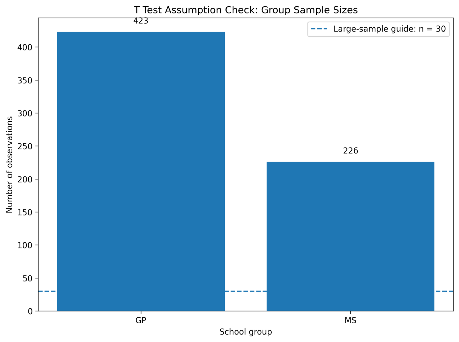
This chart checks whether the group sizes are large enough for a reliable t-test workflow. The GP group has 423 observations, and the MS group has 226 observations. Both groups are large, so the analysis is not based on tiny samples.
Large sample sizes are helpful because the t test is usually robust to moderate non-normality when each group has many observations. The uneven group sizes should still be noted, but the sample size assumption is acceptable.
Python Chart 2: G3 Distribution by Group Assumption Check
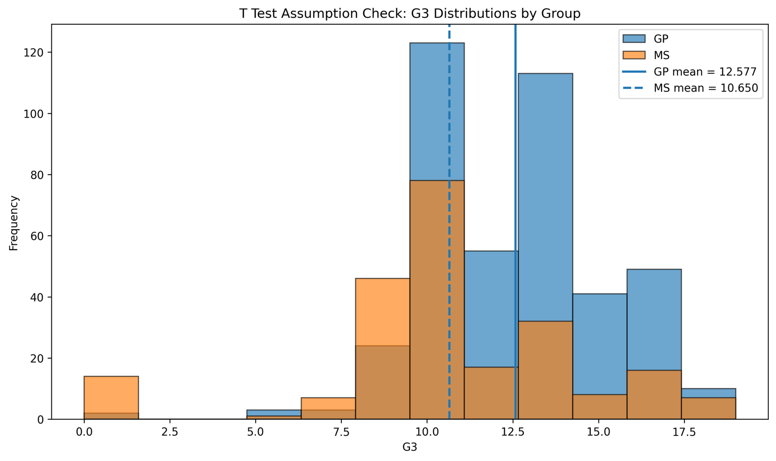
This chart examines the distribution of G3 within each school group. The two distributions are not perfectly normal, and grade data often show clustering and boundary effects. However, both groups have enough observations to make the t-test framework reasonably robust.
The chart also shows that the group centers differ and that the MS group appears more spread out. This supports checking both the mean comparison and the variance assumption.
Python Chart 3: Q-Q Plot by Group Normality Check
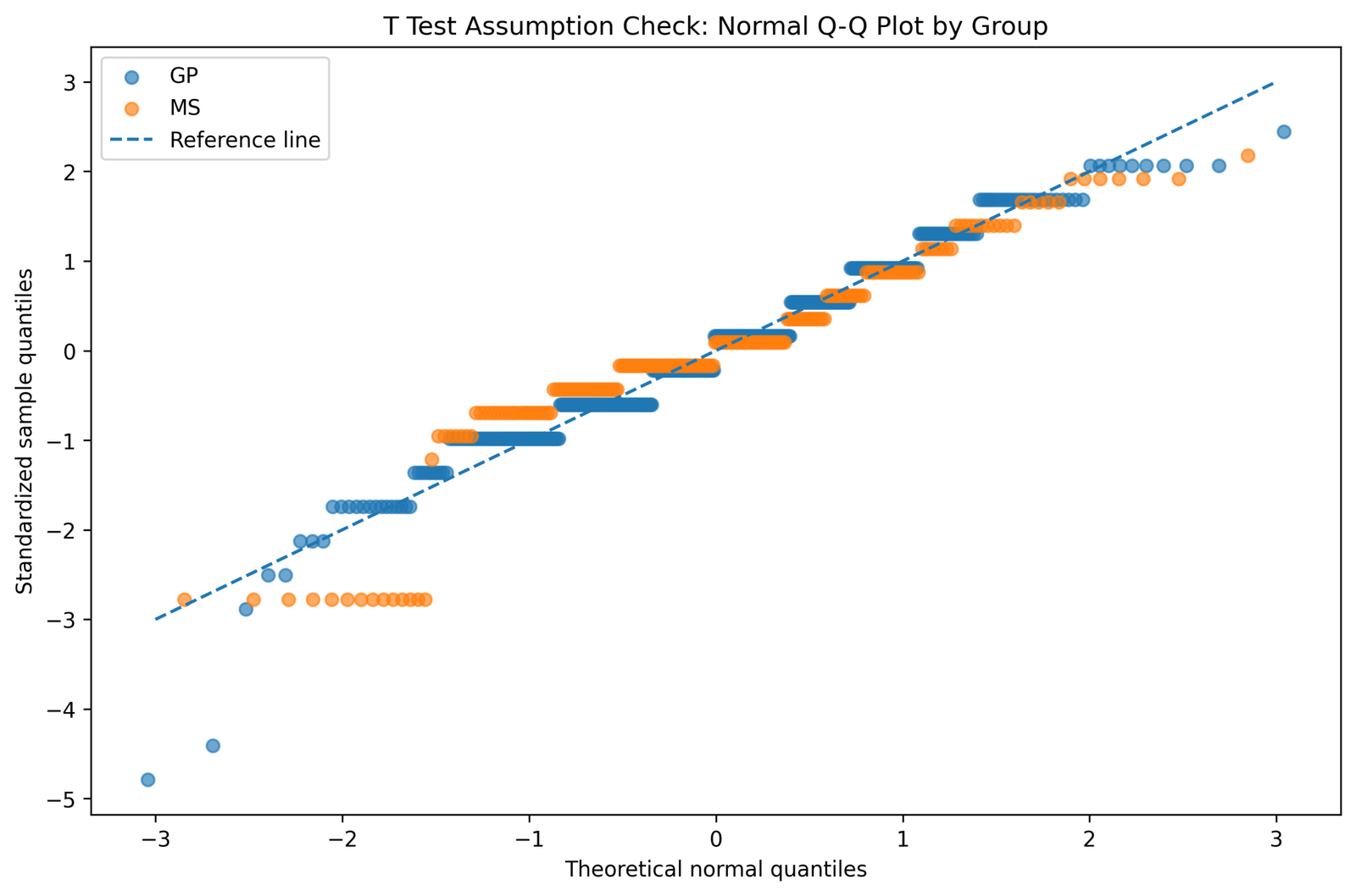
The Q-Q plot checks whether the observed values follow the expected pattern of a normal distribution. Points that follow the diagonal line closely indicate approximate normality. Points that bend away from the line show departures from normality, especially in the tails.
In this output, the normality assumption is not perfect. Tail departures should be acknowledged. However, because both groups are large, the t test can still be used with caution. If the sample were small, these departures would be more concerning.
Python Chart 4: Boxplot Outlier Check by Group
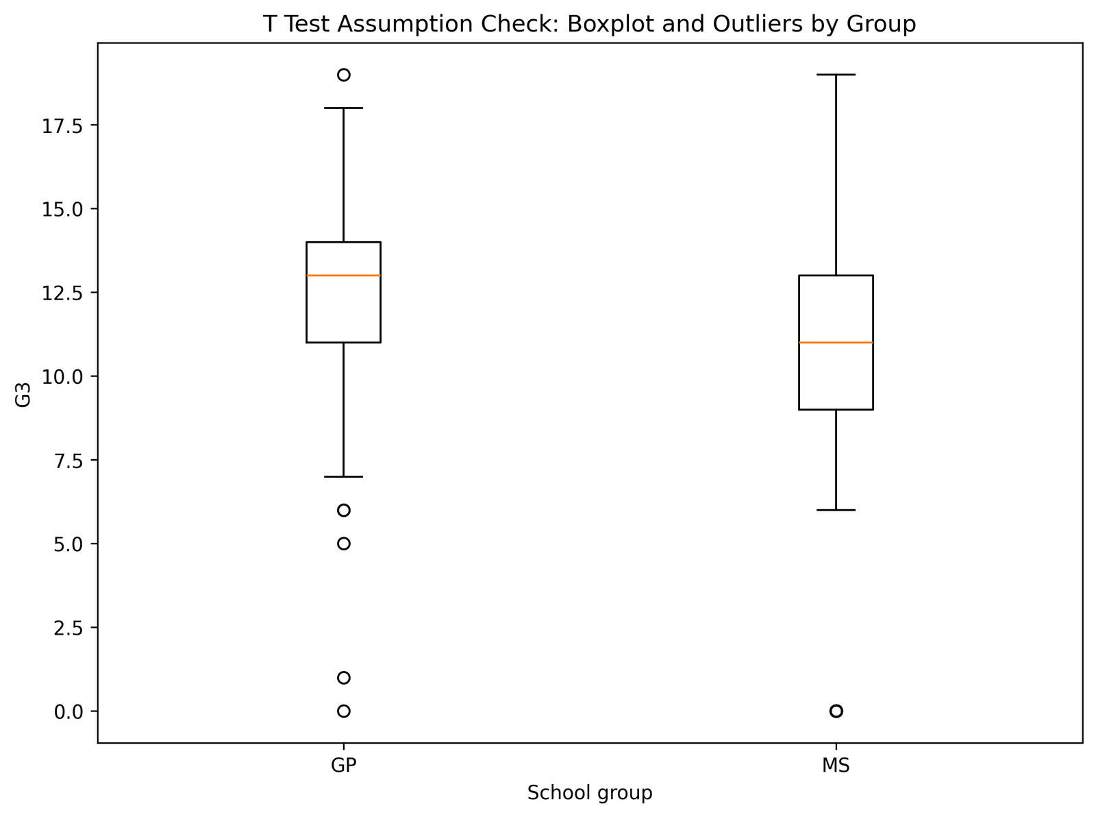
The boxplot checks for outliers and differences in spread. It shows lower-end outliers in the G3 scores. These outliers should not be ignored because extreme values can affect the mean and standard deviation.
However, the sample sizes are large, so a few outliers are less likely to overturn the entire result. The correct reporting approach is to acknowledge the outliers and, if necessary, compare the t-test result with a robust or nonparametric alternative.
Python Chart 5: Group Variance Comparison
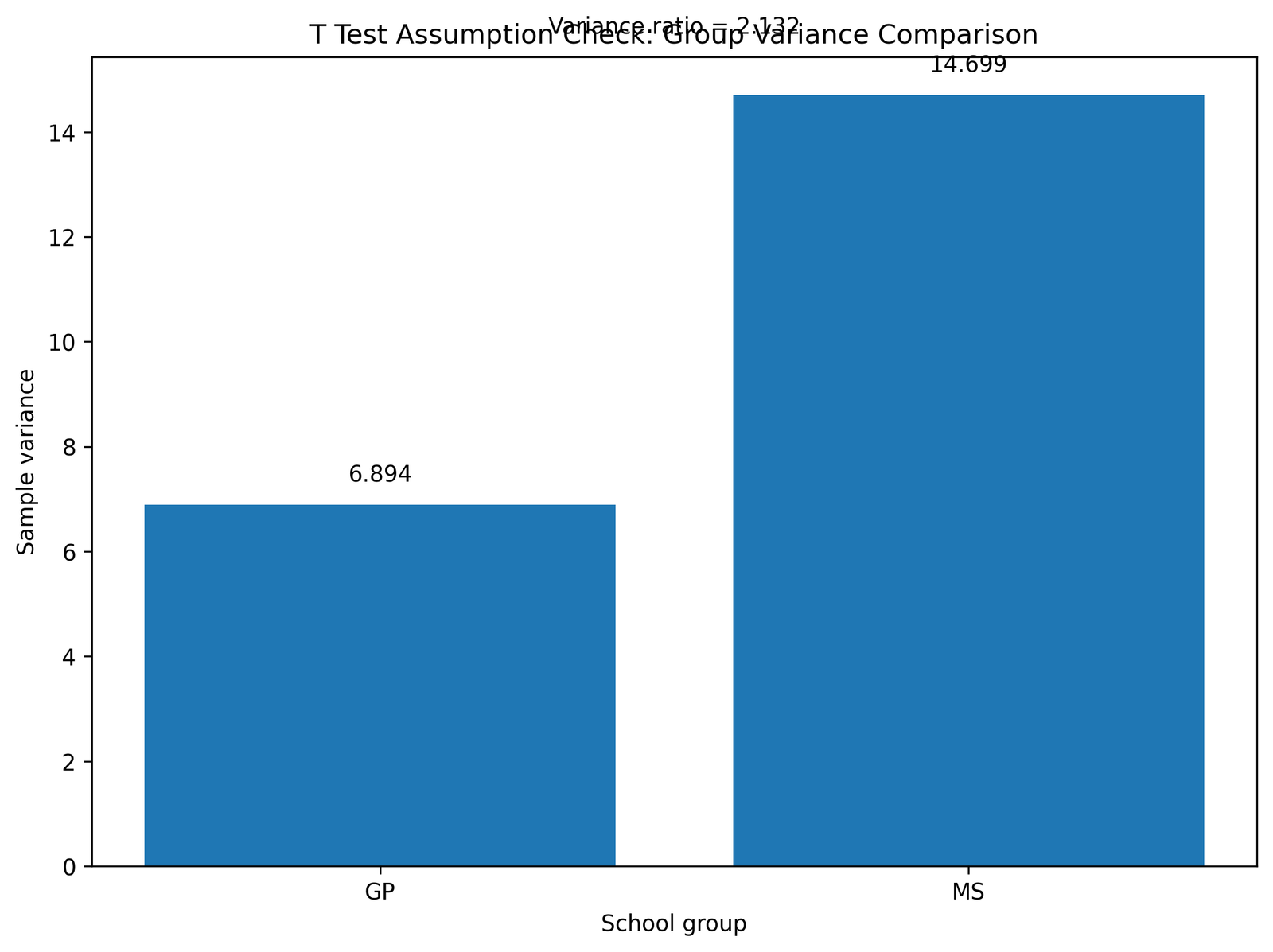
This chart checks the equal variance assumption. The MS group has more variability than the GP group. This matters because the classic Student’s t test assumes that the two groups estimate a common population variance.
The unequal spread does not mean the analysis must be abandoned. It means the analyst should check Levene’s test and consider Welch’s t test if the equal variance assumption is not supported. Welch’s t test is often safer when group variances differ.
Python Chart 6: Residuals by Group Assumption Check
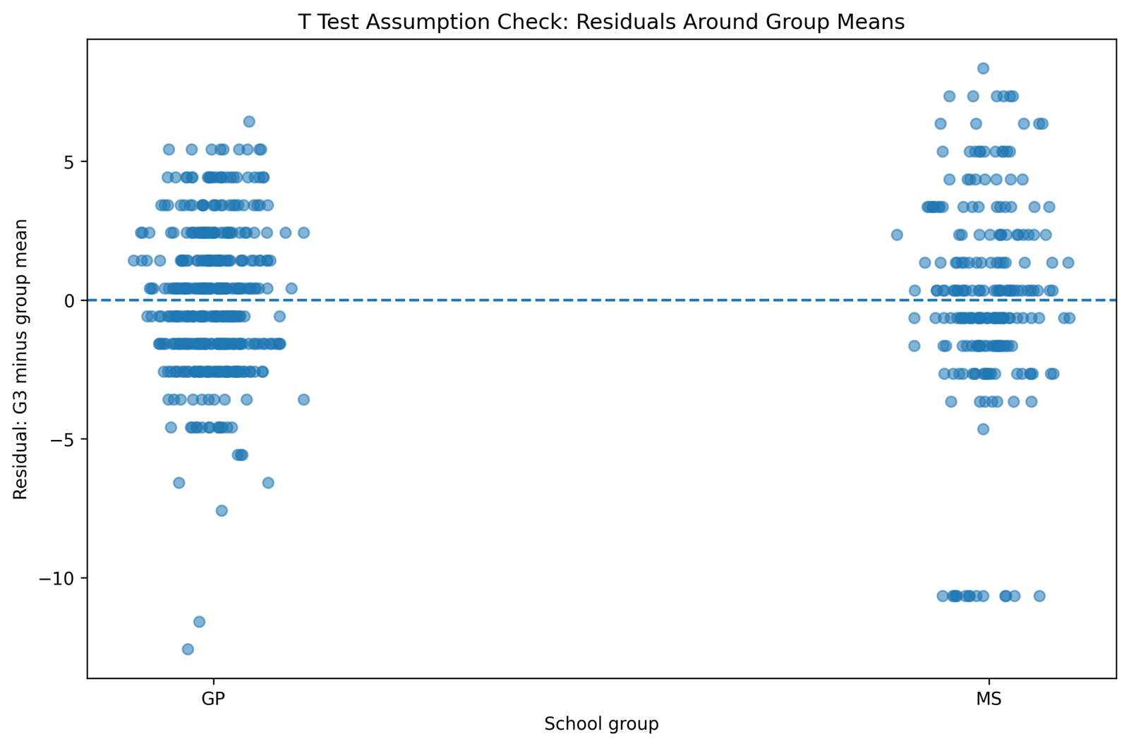
The residual chart checks how observations deviate from their group means. Good residual behavior means the deviations are centered around zero without strong structural patterns. In group comparison, residuals also reveal whether one group has much wider spread than the other.
This output supports the earlier variance caution. Residuals appear more variable for the group with greater spread. The t-test framework is still usable, but equal-variance reporting should be handled carefully.
Python Chart 7: Assumption Decision Summary
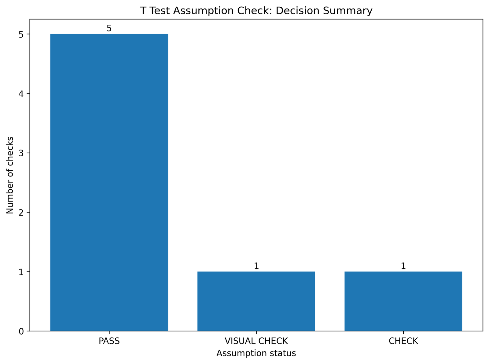
The decision summary chart brings all assumption checks together. The sample size assumption is acceptable, the numeric outcome and grouping structure are appropriate, and normality is acceptable with caution because the groups are large.
The main caution is equal variance. The variance and residual charts show that group spread is not identical. Therefore, the final recommendation is to report the assumption checks and use Welch’s t test if Levene’s test indicates unequal variances.
R Chart-by-Chart Validation
The R charts validate the Python assumption checks using a separate workflow. The same assumption pattern appears: large group sizes, moderate non-normality, visible outliers, unequal spread caution, residual spread differences and a final decision recommending careful equal-variance reporting.
R Chart 1: Group Sample Sizes for T Test
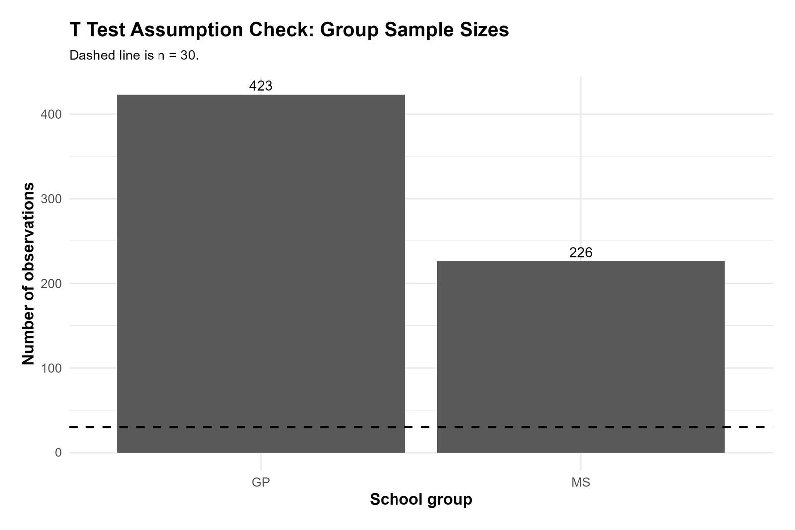
The R sample-size chart confirms that both groups are large. This is important because t tests are more robust when sample sizes are not small. The GP group has more observations than the MS group, but both groups are large enough for meaningful assumption interpretation.
The group size difference should be reported, especially because unequal group sizes can make unequal variances more influential.
R Chart 2: G3 Distribution by Group Assumption Check
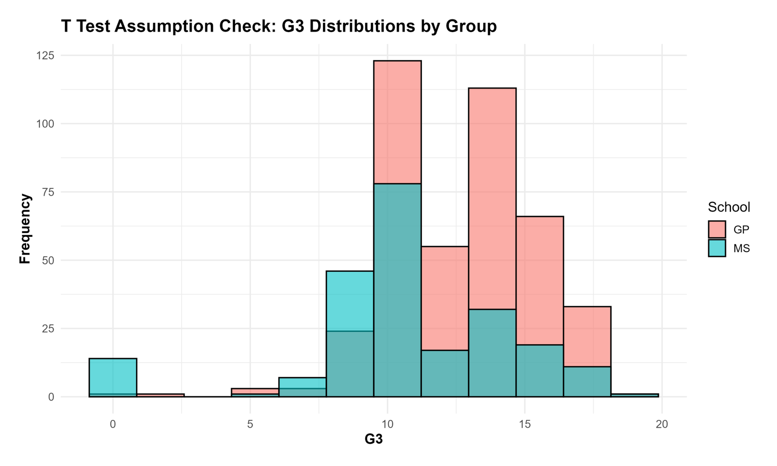
The R distribution chart confirms the distribution pattern seen in Python. The data are not perfectly normal, but the sample sizes are large. This supports the conclusion that normality is acceptable with caution rather than a reason to reject the t-test framework completely.
The chart also supports checking variance because the group spreads are not identical.
R Chart 3: Q-Q Plot by Group Normality Check
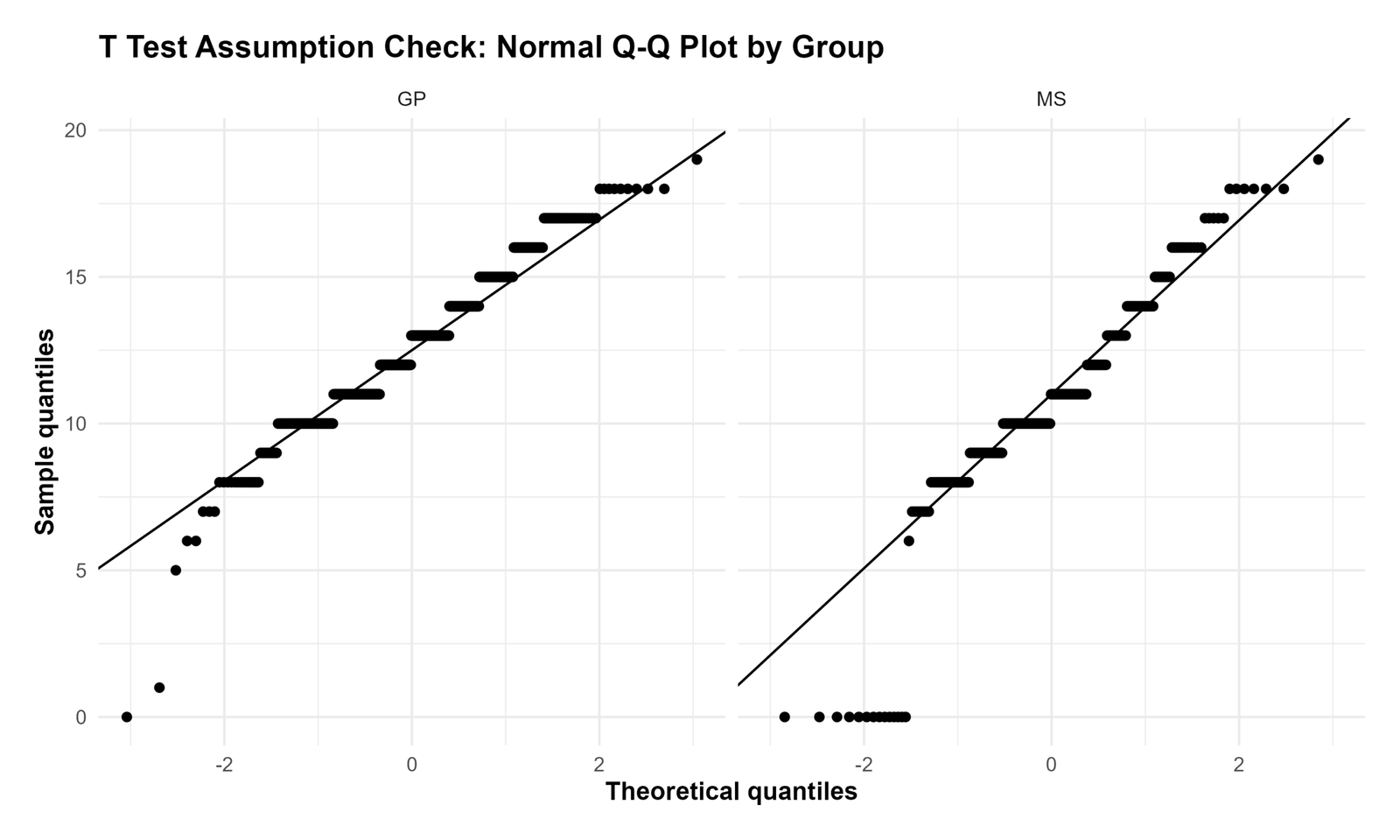
The R Q-Q plot validates the Python normality check. The central portions of the data may be acceptable, but tail departures are visible. This means the normality assumption is not perfect.
For large samples, this does not automatically prevent t-test use. The correct interpretation is cautious reporting, especially if outliers and unequal variance are also present.
R Chart 4: Boxplot Outlier Check by Group
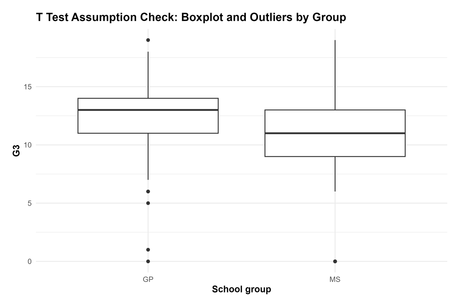
The R boxplot confirms the presence of lower-end outliers. These outliers should be reported because t tests are mean-based and means can be influenced by extreme scores.
The presence of outliers does not automatically invalidate the test, but it strengthens the need for clear assumption reporting and possible sensitivity checks.
R Chart 5: Group Variance Comparison
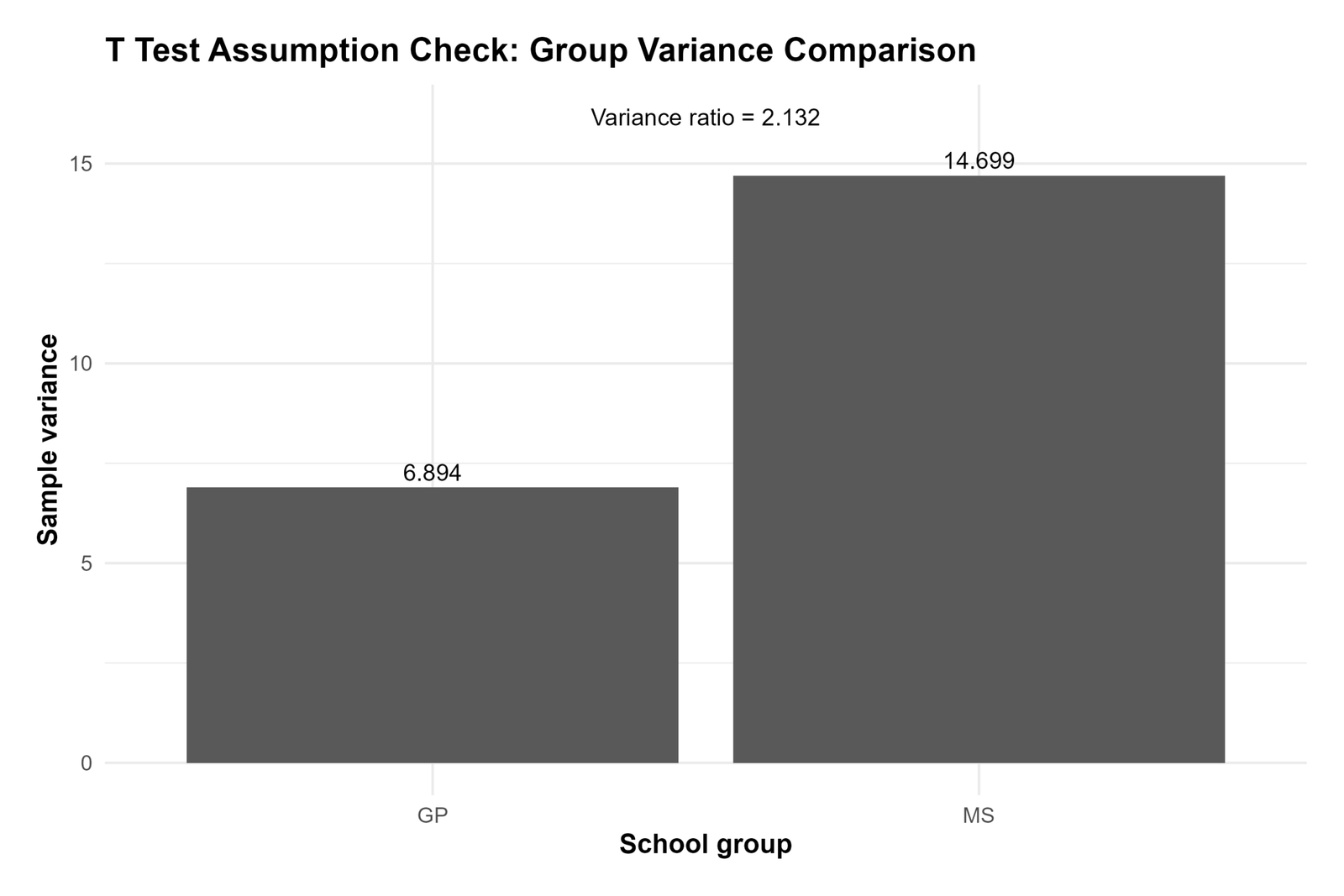
The R variance comparison confirms the main assumption caution. The MS group has a larger spread than the GP group. This affects whether the equal-variance Student’s t test row is appropriate.
If the variance difference is supported by Levene’s test, the correct reporting choice is Welch’s t test. Welch’s method adjusts the standard error and degrees of freedom for unequal variances.
R Chart 6: Residuals by Group Assumption Check
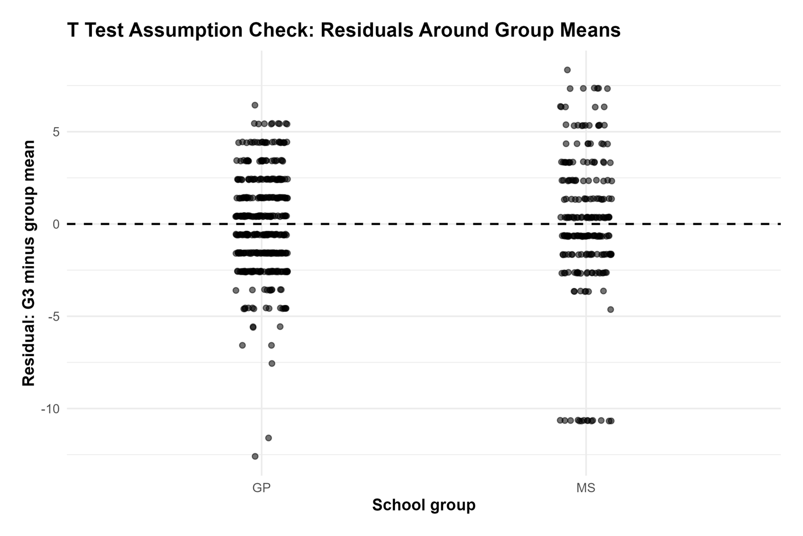
The R residual chart confirms that residual spread differs across groups. This is consistent with the variance comparison chart and supports the recommendation to check Levene’s test.
Residual diagnostics are useful because they show model behavior after subtracting the group means. If residual spread is uneven, equal-variance assumptions should be interpreted carefully.
R Chart 7: Assumption Decision Summary
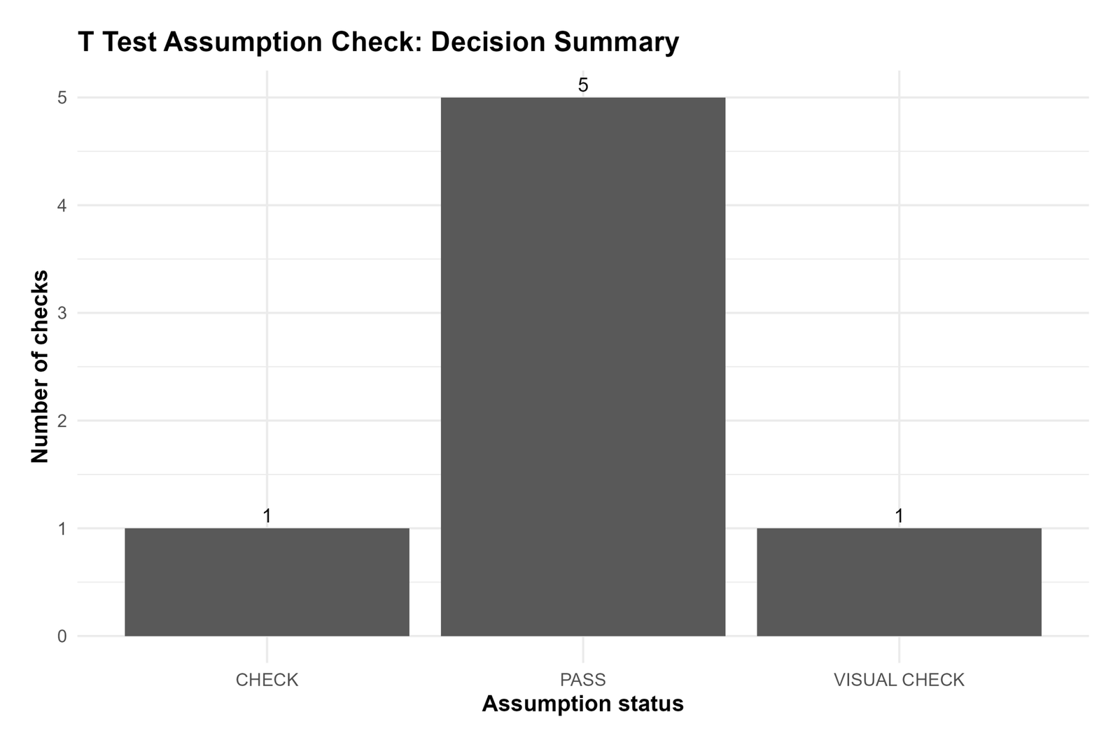
The R decision summary confirms the same final recommendation. The sample sizes and design are suitable, normality is acceptable with caution, outliers are present, and equal variance needs careful checking.
The best reporting strategy is to state the assumption findings clearly and use Welch’s t test when the equal-variance assumption is questionable.
Additional Output 1: Group Sample Sizes for T Test
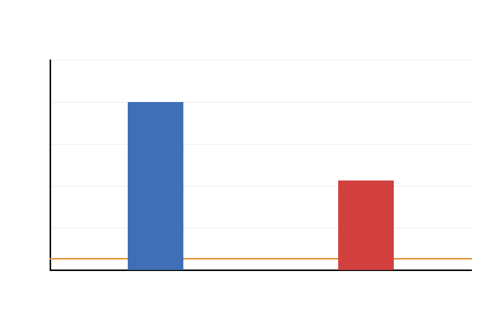
This additional output preserves the full chart set and repeats the sample-size assumption check. It confirms that both groups are large enough for robust mean comparison.
Sample size is the first practical assumption check because very small groups make normality and outlier problems more serious.
Additional Output 2: G3 Distribution by Group Assumption Check
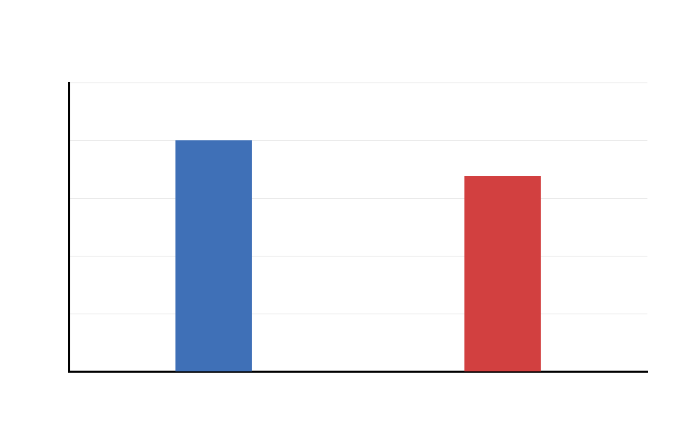
This additional distribution output confirms that normality is not perfect but is workable due to large group sizes. It also shows group-level spread differences that matter for equal-variance interpretation.
The chart should be included because distribution visuals are easier for readers to understand than normality statistics alone.
Additional Output 3: Q-Q Plot by Group Normality Check
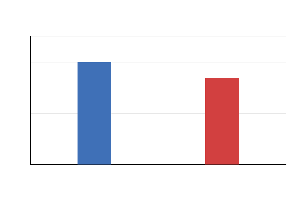
This additional Q-Q output repeats the normality check and supports the same conclusion: normality is not perfect, especially in the tails, but large samples reduce the severity of this concern.
Q-Q plots are especially useful because they show where departures from normality occur rather than giving only a single p value.
Additional Output 4: Boxplot Outlier Check by Group
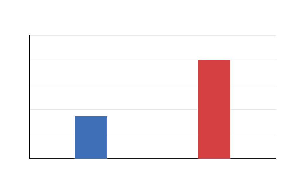
This additional boxplot output confirms the presence of lower-end outliers. Outlier checks should be part of every t-test assumption workflow because t tests compare means, and means can be pulled by extreme values.
The correct conclusion is not to delete outliers automatically. Instead, report them, verify data quality and consider sensitivity analysis if needed.
Additional Output 5: Group Variance Comparison
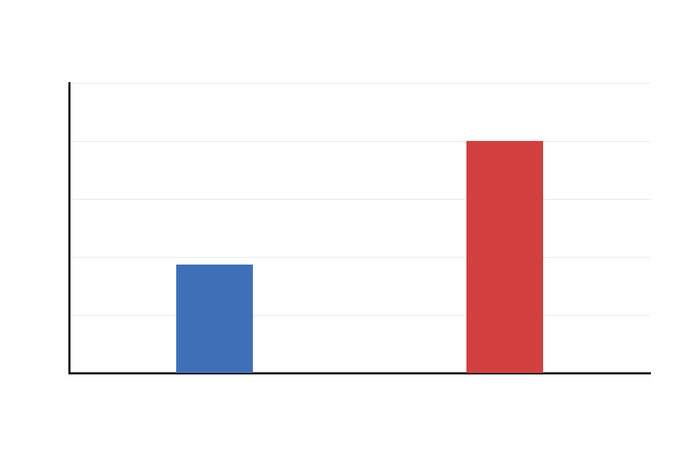
This additional variance output reinforces the equal-variance caution. The group spreads are not identical, and MS shows greater variability.
This is the main reason Welch’s t test should be considered if Levene’s test is significant or if the analyst wants a more conservative unequal-variance method.
Additional Output 6: Residuals by Group Assumption Check
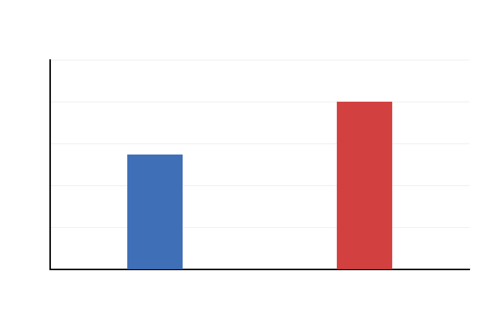
This additional residual chart supports the same diagnostic conclusion. Residuals should be centered around zero, but group spread differences can still appear.
Residual plots are helpful because they summarize model behavior after accounting for group means.
Additional Output 7: Assumption Decision Summary
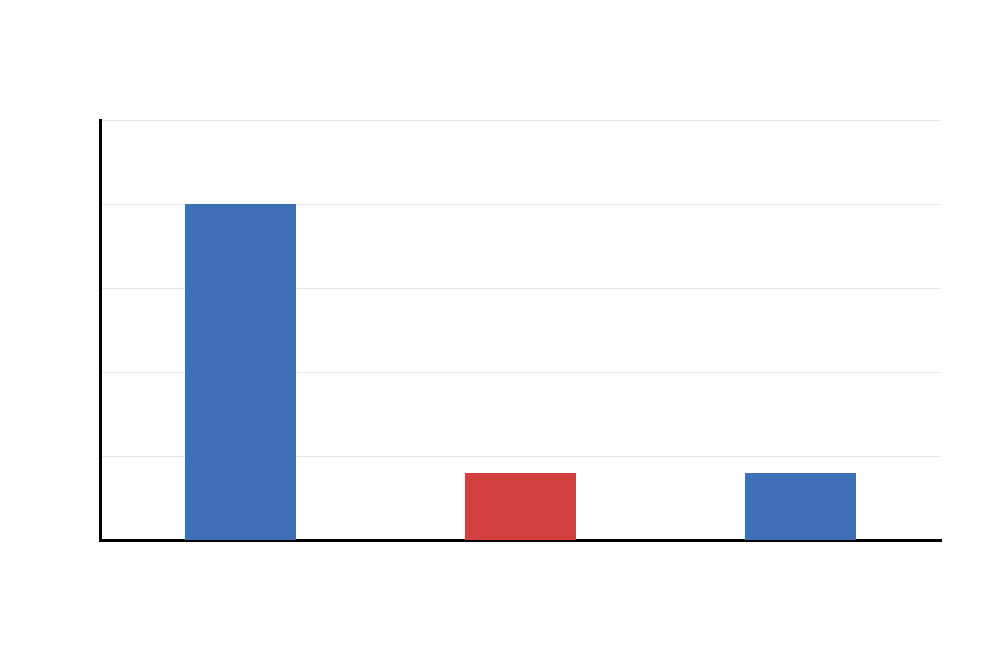
This final additional output summarizes the complete assumption workflow. It confirms that the t-test framework is usable, but equal variance should not be assumed blindly.
The best final recommendation is: report the assumptions, acknowledge outliers and non-normality, and use Welch’s t test if equal variance is not supported.
SPSS, R, Python and Excel Workflows for T Test Assumptions
The same T Test Assumptions workflow can be reproduced in SPSS, R, Python and Excel. SPSS provides Explore, Q-Q plots, boxplots and Levene’s test. Python can calculate group summaries, normality checks, Levene’s test, residuals and charts. R can produce assumption plots and run variance tests. Excel can check sample sizes, means, standard deviations, variance ratios and outliers using formulas.
SPSS Workflow
| Step | SPSS Menu or Syntax | Purpose |
|---|---|---|
| Open dataset | File > Open > Data | Load the clean dataset. |
| Check group sizes | Analyze > Descriptive Statistics > Frequencies | Confirm each group has enough cases. |
| Check distributions | Analyze > Descriptive Statistics > Explore | Create histograms, boxplots and Q-Q plots by group. |
| Check equal variance | Independent-Samples T Test output | Read Levene’s Test for Equality of Variances. |
| Choose result row | Equal variances assumed or not assumed | Use Student’s row if variance is acceptable; use Welch row if not. |
| Export output | File > Export or OUTPUT EXPORT | Save a PDF for reporting and verification. |
R Workflow
| Step | R Action | Purpose |
|---|---|---|
| Read data | read.csv() | Load the dataset. |
| Summarize groups | aggregate() or dplyr | Calculate n, mean, SD and variance by group. |
| Check normality | Q-Q plots and Shapiro checks | Inspect distribution shape within groups. |
| Check outliers | boxplot() or IQR rules | Identify extreme values. |
| Check variance | var.test() or Levene’s test | Evaluate equality of variance. |
| Choose t test | t.test(..., var.equal=TRUE/FALSE) | Run Student’s or Welch’s t test. |
Python Workflow
| Step | Python Action | Purpose |
|---|---|---|
| Read data | pandas.read_csv() | Load the dataset into a DataFrame. |
| Summarize groups | groupby().agg() | Calculate group size, mean, SD and variance. |
| Check normality | scipy.stats.probplot() | Create Q-Q plots by group. |
| Check outliers | IQR method and boxplots | Detect extreme values. |
| Check variance | scipy.stats.levene() | Run Levene’s test. |
| Choose test | ttest_ind(equal_var=True/False) | Run Student’s or Welch’s t test. |
Excel Workflow
| Excel Task | Formula or Tool | Purpose |
|---|---|---|
| Calculate sample sizes | =COUNT(range) | Check group sizes. |
| Calculate means | =AVERAGE(range) | Understand group centers. |
| Calculate standard deviations | =STDEV.S(range) | Compare group spread. |
| Calculate variance ratio | =MAX(var1,var2)/MIN(var1,var2) | Screen equal variance assumption. |
| Check outliers | Quartiles and IQR fences | Identify unusually low or high values. |
| Create visuals | Histograms, boxplots and scatter plots | Support visual assumption reporting. |
Code Blocks for T Test Assumptions
SPSS Syntax for T Test Assumptions
* T Test Assumptions in SPSS.
* Outcome variable: G3.
* Grouping variable: school.
* Groups: GP and MS.

TITLE "T Test Assumptions: G3 by School".

FREQUENCIES VARIABLES=school.

EXAMINE VARIABLES=G3 BY school
  /PLOT BOXPLOT HISTOGRAM NPPLOT
  /COMPARE GROUPS
  /STATISTICS DESCRIPTIVES
  /CINTERVAL 95
  /MISSING LISTWISE
  /NOTOTAL.

T-TEST GROUPS=school('GP' 'MS')
  /VARIABLES=G3
  /MISSING=ANALYSIS
  /CRITERIA=CI(.95).

MEANS TABLES=G3 BY school
  /CELLS MEAN COUNT STDDEV VARIANCE SEMEAN.

OUTPUT EXPORT
  /CONTENTS EXPORT=VISIBLE
  /PDF DOCUMENTFILE="T-Test-Assumptions-SPSS-Output.pdf".
Python Code for T Test Assumptions
import pandas as pd
import numpy as np
from scipy import stats

df = pd.read_csv("dataset.csv")

data = df[["school", "G3"]].copy()
data["G3"] = pd.to_numeric(data["G3"], errors="coerce")
data = data.dropna(subset=["school", "G3"])

gp = data.loc[data["school"] == "GP", "G3"]
ms = data.loc[data["school"] == "MS", "G3"]

summary = data.groupby("school")["G3"].agg(["count", "mean", "std", "var"])
print(summary)

# Sample size check
print("GP n:", len(gp))
print("MS n:", len(ms))

# Variance ratio
var_gp = gp.var(ddof=1)
var_ms = ms.var(ddof=1)
variance_ratio = max(var_gp, var_ms) / min(var_gp, var_ms)
print("Variance ratio:", variance_ratio)

# Levene test for homogeneity of variance
levene_stat, levene_p = stats.levene(gp, ms, center="median")
print("Levene statistic:", levene_stat)
print("Levene p-value:", levene_p)

# Normality checks
# Shapiro can be overly sensitive with large samples, so interpret with plots too.
shapiro_gp = stats.shapiro(gp.sample(min(len(gp), 500), random_state=1))
shapiro_ms = stats.shapiro(ms.sample(min(len(ms), 500), random_state=1))
print("Shapiro GP:", shapiro_gp)
print("Shapiro MS:", shapiro_ms)

# Outlier counts using IQR
def iqr_outlier_count(x):
    q1 = x.quantile(0.25)
    q3 = x.quantile(0.75)
    iqr = q3 - q1
    low = q1 - 1.5 * iqr
    high = q3 + 1.5 * iqr
    return ((x < low) | (x > high)).sum(), low, high

print("GP outliers:", iqr_outlier_count(gp))
print("MS outliers:", iqr_outlier_count(ms))

# Residuals by group
group_means = data.groupby("school")["G3"].transform("mean")
data["residual"] = data["G3"] - group_means
print(data.groupby("school")["residual"].agg(["mean", "std", "min", "max"]))

# Test choice logic
if levene_p < 0.05:
    print("Recommendation: Use Welch's t test because variance equality is questionable.")
else:
    print("Recommendation: Equal-variance Student's t test is acceptable.")
R Code for T Test Assumptions
# T Test Assumptions in R

df <- read.csv("dataset.csv")

df$G3 <- as.numeric(df$G3)
df$school <- as.factor(df$school)

df_model <- na.omit(df[, c("school", "G3")])

# Group summaries
print(aggregate(G3 ~ school, data = df_model,
                FUN = function(x) c(n = length(x),
                                    mean = mean(x),
                                    sd = sd(x),
                                    var = var(x))))

gp <- df_model$G3[df_model$school == "GP"]
ms <- df_model$G3[df_model$school == "MS"]

# Variance ratio
variance_ratio <- max(var(gp), var(ms)) / min(var(gp), var(ms))
cat("Variance ratio =", variance_ratio, "\n")

# F test for variance comparison
print(var.test(gp, ms))

# Levene test if car package is available
# install.packages("car")
# library(car)
# print(leveneTest(G3 ~ school, data = df_model))

# Normality checks
qqnorm(gp, main = "Q-Q Plot GP")
qqline(gp)

qqnorm(ms, main = "Q-Q Plot MS")
qqline(ms)

# Boxplots
boxplot(G3 ~ school, data = df_model,
        main = "G3 Boxplot by School",
        xlab = "School",
        ylab = "G3")

# Residuals by group
df_model$residual <- df_model$G3 - ave(df_model$G3, df_model$school)
print(aggregate(residual ~ school, data = df_model,
                FUN = function(x) c(mean = mean(x),
                                    sd = sd(x),
                                    min = min(x),
                                    max = max(x))))

# Compare Student and Welch versions
print(t.test(G3 ~ school, data = df_model, var.equal = TRUE))
print(t.test(G3 ~ school, data = df_model, var.equal = FALSE))
Excel Formulas for T Test Assumptions
Step 1:
Place GP G3 values in one column and MS G3 values in another column.

Step 2:
Calculate sample sizes:
=COUNT(GP_range)
=COUNT(MS_range)

Step 3:
Calculate group means:
=AVERAGE(GP_range)
=AVERAGE(MS_range)

Step 4:
Calculate group standard deviations:
=STDEV.S(GP_range)
=STDEV.S(MS_range)

Step 5:
Calculate group variances:
=VAR.S(GP_range)
=VAR.S(MS_range)

Step 6:
Calculate variance ratio:
=MAX(GP_variance,MS_variance)/MIN(GP_variance,MS_variance)

Step 7:
Calculate quartiles:
=QUARTILE.INC(range,1)
=QUARTILE.INC(range,3)

Step 8:
Calculate IQR:
=Q3-Q1

Step 9:
Calculate lower outlier fence:
=Q1-1.5*IQR

Step 10:
Calculate upper outlier fence:
=Q3+1.5*IQR

Step 11:
Create charts:
- Histogram by group
- Q-Q plot manually using normal quantiles
- Boxplot by group
- Variance comparison chart
- Residual plot by group

Step 12:
Decision:
If sample sizes are large and normality is only moderately imperfect, t test is usually robust.
If variances differ strongly, use Welch's t test instead of equal-variance Student's t test.
APA Reporting Wording for T Test Assumptions
T Test Assumptions should be reported before or alongside the final t test result. The report should mention sample sizes, distribution checks, outliers and variance equality. If Welch's test is used, explain that it was selected because the equal variance assumption was questionable.
APA example: Prior to conducting the independent-samples t test, assumptions were evaluated using group sample sizes, histograms, Q-Q plots, boxplots, variance comparison and residual plots. The groups were large (GP n = 423, MS n = 226), supporting robustness to moderate non-normality. Q-Q plots and histograms showed some departure from normality, and boxplots indicated lower-end outliers. Group spread differed, with MS showing greater variability than GP; therefore, the equal-variance assumption was treated with caution and Welch's t test was considered when appropriate.
Short reporting version: Assumption checks showed large group sample sizes and acceptable normality with caution. Outliers were present, and group variances differed, so Welch's t test should be used if Levene's test indicates unequal variances.
Common Mistakes in T Test Assumptions
| Mistake | Why It Is a Problem | Correct Practice |
|---|---|---|
| Ignoring independence | No assumption check can fix a wrong study design. | Choose independent, paired or one-sample t test based on design. |
| Using only Shapiro-Wilk p value | Large samples often make small deviations statistically significant. | Use histograms, Q-Q plots and sample size context. |
| Deleting outliers automatically | Outliers may be real observations. | Check data quality, report outliers and consider sensitivity analysis. |
| Assuming equal variances without checking | Unequal variances can affect the standard Student's t test. | Use Levene's test and consider Welch's t test. |
| Confusing normality of raw scores with normality of means | The t test is often robust with large samples. | Interpret normality in relation to sample size and design. |
| Reporting assumptions separately from the final test choice | The reader cannot see how assumptions affected the analysis. | State whether Student's or Welch's t test was used and why. |
When to Use T Test Assumptions
Use T Test Assumptions checks before every t test. The exact checks depend on the design, but the purpose is always the same: confirm that the chosen t-test method matches the data structure and that the result can be interpreted responsibly.
| T Test Type | Main Assumptions | What to Check |
|---|---|---|
| One sample t test | Numeric variable, independent observations, normality or large sample. | Histogram, Q-Q plot, outliers and sample size. |
| Independent samples t test | Two independent groups, numeric outcome, normality, equal variance if using Student's t test. | Group sizes, distributions, Q-Q plots, boxplots, Levene's test. |
| Paired t test | Paired observations and normality of difference scores. | Difference-score histogram, Q-Q plot and outliers. |
| Welch's t test | Two independent groups and numeric outcome. | Used when variances are unequal or group sizes differ. |
Do not skip assumptions just because software gives a p value. Software will run the test, but the analyst must decide whether the test choice is appropriate.
Downloads and Resources
Use the following downloadable resources to reproduce the T Test Assumptions workflow in SPSS, Python, R and Excel. Replace the placeholder links with the final hosted file URLs after uploading your scripts and templates to WordPress Media Library.
Download SPSS Syntax
T Test Assumptions syntax with Explore, Q-Q plots, boxplots, Levene output and PDF export.
Download Python Script
Python workflow with sample sizes, normality plots, outlier checks, variance checks and residual charts.
Download R Script
R workflow with Q-Q plots, boxplots, variance checks, residual diagnostics and t-test comparison.
Download Excel Template
Excel formulas for sample size, SD, variance ratio, IQR outliers and assumption decision checklist.
FAQs About T Test Assumptions
What are T Test Assumptions?
T Test Assumptions are the conditions that should be checked before interpreting a t test. They usually include independent observations, a numeric outcome, approximate normality or large sample size, outlier checks and equal variance for the standard independent samples t test.
What assumptions were checked in this example?
This example checked group sample sizes, G3 distribution by group, Q-Q plots, boxplot outliers, group variance comparison, residuals by group and an overall assumption decision summary.
Are the T Test Assumptions acceptable in this example?
The assumptions are mostly acceptable with caution. Sample sizes are large, normality is acceptable with caution, outliers are present, and equal variance is the main concern because MS has more variability than GP.
What should I do if equal variance is violated?
If equal variance is not supported, use Welch's t test instead of the equal-variance Student's t test. Welch's t test adjusts the standard error and degrees of freedom for unequal variances.
Does a t test require perfectly normal data?
No. The t test is often robust to moderate non-normality when sample sizes are large. However, severe skewness, extreme outliers or very small samples require more caution.
How do I check T Test Assumptions in SPSS?
Use Explore for histograms, Q-Q plots and boxplots. Use the Independent-Samples T Test output to read Levene's test and choose either the equal-variance row or the unequal-variance Welch row.
Can I check T Test Assumptions in Excel?
Yes. Excel can check sample sizes, means, standard deviations, variances, variance ratios and IQR outliers. It can also create histograms and boxplots for visual assumption checking.

