
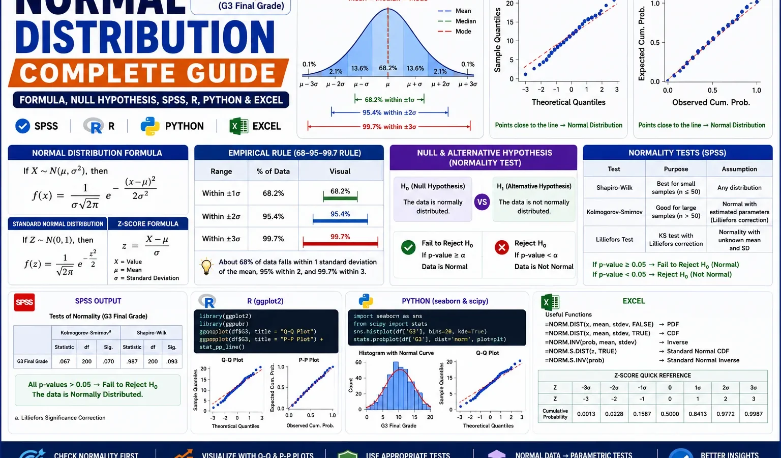
Normality Test, Bell Curve, Q-Q Plot, P-P Plot and Z-Score Guide
Normal distribution is the bell-shaped probability distribution used in many statistical tests, confidence intervals and regression assumptions. This guide explains the normal distribution formula, null hypothesis, alternative hypothesis, SPSS normality tests, Python charts, R charts, Q-Q plot, P-P plot, z-scores, empirical rule and Excel workflow using G3 final grade from the student-por.csv dataset.
Quick Answer: Is G3 Normally Distributed?
The normal distribution check for G3 final grade does not support normality. The SPSS output reports N = 649, mean = 11.91, standard deviation = 3.231, skewness = -0.913 and kurtosis = 2.712. The formal normality tests also reject normality: Kolmogorov-Smirnov statistic = .124, df = 649, p = .000 and Shapiro-Wilk statistic = .926, df = 649, p = .000. In SPSS reporting, p = .000 should be written as p < .001, not as an exact zero.
Null hypothesis: G3 final grade follows a normal distribution. Alternative hypothesis: G3 final grade does not follow a normal distribution. Because both normality tests have p < .001, we reject the null hypothesis. The histogram, Q-Q plot, P-P plot, z-score distribution and empirical rule check all support the same practical decision: G3 is approximately centered around 12, but it has a low-score tail, heavy-tail behavior and clear deviation from a perfect normal bell curve.
Final normality decision: Reject the normality null hypothesis. G3 is not normally distributed according to the Kolmogorov-Smirnov and Shapiro-Wilk tests. The visual charts show why: there are many central scores around 10 to 15, but there are also very low scores near 0 that pull the left tail away from a normal curve.
Table of Contents
- What Is Normal Distribution?
- Normal Distribution Formula
- Null and Alternative Hypothesis for Normal Distribution
- Dataset and SPSS-Ready Files Used
- Verified SPSS Normal Distribution Results
- Python Charts and Full Interpretation
- R Validation Charts
- How to Check Normal Distribution in Python, R, SPSS and Excel
- How to Report the Normal Distribution Decision
- Common Mistakes
- Download SPSS Output
- FAQs
What Is Normal Distribution?
A normal distribution is a continuous, bell-shaped distribution where values are symmetrically distributed around the mean. In an ideal normal distribution, the mean, median and mode are equal, the curve is balanced on both sides, and most values are close to the center. The standard normal distribution is a special normal distribution with mean = 0 and standard deviation = 1.
Normal distribution is important because many statistical methods assume that the outcome, residuals or sampling distribution is approximately normal. It affects how we interpret confidence intervals, one-sample tests, regression diagnostics and assumption checks. However, real datasets rarely look perfectly normal. That is why analysts should combine formal normality tests with visual checks such as a Q-Q plot normality check, P-P plot normality check, histogram interpretation and box plot interpretation.
In this worked example, G3 final grade has a mean of 11.91 and a standard deviation of 3.231. The center is clear, but the distribution is not perfectly normal because low scores near 0 create a left-tail problem. This is also visible in the z-score range, where the minimum standardized value is -3.69 and the maximum is only 2.20. A perfectly normal distribution would usually show a more balanced tail pattern.
Simple meaning: Normal distribution means a bell-shaped pattern. Most values are near the mean, fewer values appear far away from the mean, and the left and right tails should be roughly balanced. For G3, the bell shape is only partial because the left tail is too strong.
Normal Distribution Formula
The probability density function of a normal distribution is written as:
f(x) = [1 / (σ√(2π))] × e^[-(x - μ)² / (2σ²)]| Symbol | Meaning | G3 example |
|---|---|---|
| x | A specific observed value | A G3 score such as 10, 11, 12 or 13 |
| μ | Mean of the distribution | 11.91 |
| σ | Standard deviation | 3.231 |
| π | Mathematical constant pi | Used in the curve formula |
| e | Natural exponential constant | Used to create the bell curve shape |
The standard normal distribution uses z-scores. A z-score tells how many standard deviations an observed value is from the mean:
z = (x - mean) / standard deviationFor example, a G3 score of 0 is far below the mean. Using the SPSS output values, its approximate z-score is (0 – 11.91) / 3.231 = -3.69. This is a very low standardized value and explains why the left tail creates a normality problem. A G3 score of 19 has a z-score of about 2.20, which is high but not as extreme as the low-score tail.
Null and Alternative Hypothesis for Normal Distribution
A normality test uses a formal hypothesis decision. This is important for SEO and for statistical reporting because readers often search for “normal distribution null hypothesis,” “normality test alternative hypothesis,” or “reject the null hypothesis for normal distribution.”
| Hypothesis | Statement | Meaning for G3 final grade |
|---|---|---|
| Null hypothesis | H0: G3 is normally distributed. | The observed G3 values are consistent with a normal bell curve. |
| Alternative hypothesis | H1: G3 is not normally distributed. | The observed G3 values differ significantly from a normal bell curve. |
| Decision rule | If p < .05, reject H0. | A significant Kolmogorov-Smirnov or Shapiro-Wilk result means normality is rejected. |
| SPSS result | K-S p = .000; Shapiro-Wilk p = .000 | Report both as p < .001. |
| Final decision | Reject H0 | G3 does not follow a normal distribution. |
Hypothesis decision: The null hypothesis of normality is rejected for G3 final grade. The result is statistically significant in both Kolmogorov-Smirnov and Shapiro-Wilk tests. This means the observed G3 distribution differs from the expected normal distribution.
Practical caution: With a large sample such as N = 649, formal normality tests can detect small deviations. Therefore, do not rely on p-values alone. Read the result together with the histogram, Q-Q plot, P-P plot, z-score distribution and empirical rule check. For more normality methods, see the Kolmogorov-Smirnov test, Lilliefors test, DAgostino Pearson test, Ryan-Joiner test and Cramer-von Mises test.
Dataset and SPSS-Ready Files Used
This guide uses the student-por.csv dataset. The main variable is G3 final grade. Python and R were used to generate visual checks, while SPSS was used to verify descriptive statistics, Kolmogorov-Smirnov normality results, Shapiro-Wilk normality results, z-scores and empirical rule frequencies.
| Item | Value or file | Purpose |
|---|---|---|
| Main dataset | student-por.csv | Student performance data used for the normal distribution example. |
| Main variable | G3 final grade | Outcome checked for normality. |
| Valid cases | 649 | No missing G3 cases in the SPSS output. |
| SPSS output | Normal-Distribution-SPSS-Output.pdf | Confirms descriptive statistics, normality tests, z-scores and empirical rule counts. |
| Python charts | 5 charts | Normal curve histogram, Q-Q plot, P-P plot, z-score histogram and empirical rule chart. |
| R charts | 5 charts | Independent R validation of the same visual normality checks. |
External dataset source: UCI Machine Learning Repository: Student Performance dataset.
Verified SPSS Normal Distribution Results
The SPSS output gives the most important normal distribution statistics for G3 final grade. The distribution has a clear center around 12, but the skewness, kurtosis, formal normality tests and low-end z-scores show that it is not a perfect normal distribution.
Descriptive Statistics for G3
| Statistic | SPSS value | Normal distribution interpretation |
|---|---|---|
| N | 649 | The normality check used 649 valid G3 scores. |
| Mean | 11.91 | The fitted normal curve is centered at 11.91. |
| Median | 12.00 | The middle score is close to the mean, so the center is clear. |
| Mode | 11 | The most frequent score is 11. |
| Standard deviation | 3.231 | Used to fit the normal curve and calculate z-scores. |
| Variance | 10.437 | The squared spread of G3 scores. |
| Minimum | 0 | Very low value creating a left-tail deviation. |
| Maximum | 19 | Highest observed grade. |
| Range | 19 | G3 spans from 0 to 19. |
| Interquartile range | 4 | The middle 50% of G3 values covers about four grade points. |
| Skewness | -0.913 | Negative skewness shows a low-score tail. |
| Kurtosis | 2.712 | Positive excess kurtosis suggests heavier tails or sharper concentration than a normal distribution. |
SPSS Tests of Normality
| Normality test | Statistic | df | Sig. | Decision |
|---|---|---|---|---|
| Kolmogorov-Smirnov with Lilliefors correction | .124 | 649 | .000 | Reject H0; G3 is not normally distributed. |
| Shapiro-Wilk | .926 | 649 | .000 | Reject H0; G3 is not normally distributed. |
The Kolmogorov-Smirnov test compares the observed cumulative distribution with a theoretical normal distribution. The Shapiro-Wilk test is another formal test of normality. Both tests have p < .001, so the normality null hypothesis is rejected. This result should be reported clearly, but it should not be interpreted without the visual checks because large datasets can make small distribution differences statistically significant.
G3 Frequency Table Pattern
| G3 score | Frequency | Percent | Normality meaning |
|---|---|---|---|
| 0 | 15 | 2.3% | Creates a strong low-end tail and a very negative z-score. |
| 10 | 97 | 14.9% | Dense central grade region. |
| 11 | 104 | 16.0% | Most frequent score and major central peak. |
| 12 | 72 | 11.1% | Close to the median and fitted normal center. |
| 13 | 82 | 12.6% | Another dense central grade value. |
| 19 | 2 | 0.3% | High-end value, but less extreme than the low-score tail. |
Z-Score and Empirical Rule Results
| Band | Observed proportion | Normal expected proportion | Interpretation |
|---|---|---|---|
| Mean ± 1 SD | 0.773 | 0.683 | More G3 values than expected are packed near the center. |
| Mean ± 2 SD | 0.971 | 0.955 | Slightly more values than expected fall within two standard deviations. |
| Mean ± 3 SD | 0.975 | 0.997 | Fewer values than expected fall within three standard deviations because 16 low-score cases fall outside the band. |
The empirical rule check is one of the most practical ways to explain the normal distribution result. A normal distribution should have about 68.3% of values within one standard deviation, 95.5% within two standard deviations and 99.7% within three standard deviations. For G3, the one-standard-deviation and two-standard-deviation bands are higher than normal expectation, but the three-standard-deviation band is lower because the low score of 0 has a z-score of about -3.69. This is another reason the final decision is to reject the normality null hypothesis.
Python Charts and Full Interpretation
1. Normal Distribution Histogram Curve for G3
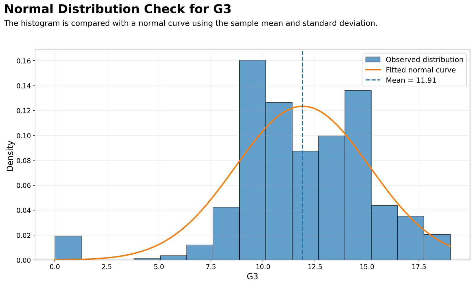
This histogram compares the observed G3 distribution with a fitted normal curve. The blue bars show the observed density of G3 scores, the orange curve shows the normal distribution expected from the sample mean and standard deviation, and the dashed vertical line marks the mean at about 11.91. The central part of the distribution is concentrated between about 10 and 15, so the fitted normal curve captures the broad location of the data. However, the histogram does not follow the curve perfectly. There is a visible bar near 0, showing very low final grades that are much farther left than a clean normal bell curve would expect. The bars around 10 to 11 and 14 to 15 are also uneven, suggesting a discrete grade distribution rather than a smooth continuous normal distribution. This chart supports the formal hypothesis decision: the distribution has a central bell-like region, but the low-score tail and uneven grade clustering mean we reject the null hypothesis of perfect normality.
2. Q-Q Plot for G3
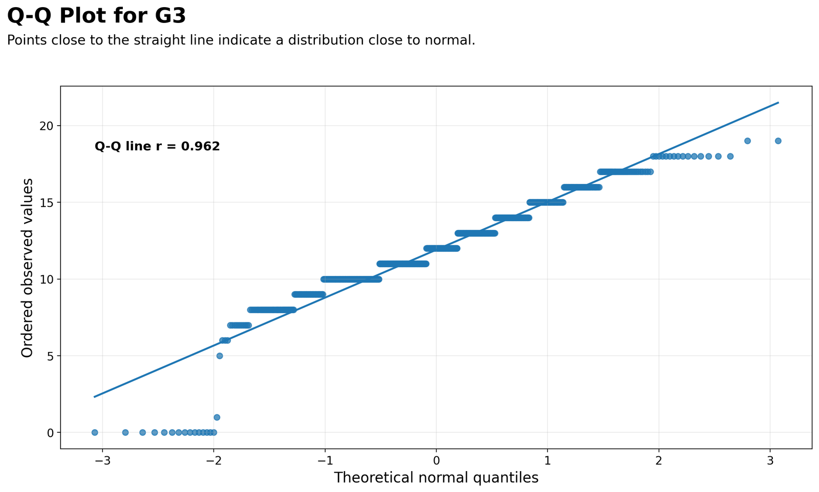
The Q-Q plot checks whether the ordered observed G3 values follow the theoretical quantiles of a normal distribution. If G3 were normally distributed, the points would sit close to the diagonal reference line across the full range. The chart reports a Q-Q line correlation of about r = 0.962, which means the middle of the distribution has a fairly strong linear pattern. However, normality is not judged only by the middle. The left tail shows clear deviation because many low values sit far away from the reference line, especially around score 0. The upper tail also flattens because G3 is bounded at the high end and has only a few scores near 18 and 19. The stepped pattern occurs because G3 is an integer grade variable rather than a continuous measurement. This chart shows partial normal-like behavior in the center but non-normal behavior in the tails. Therefore, it agrees with the SPSS Kolmogorov-Smirnov and Shapiro-Wilk results: reject the normality null hypothesis.
3. P-P Plot for G3
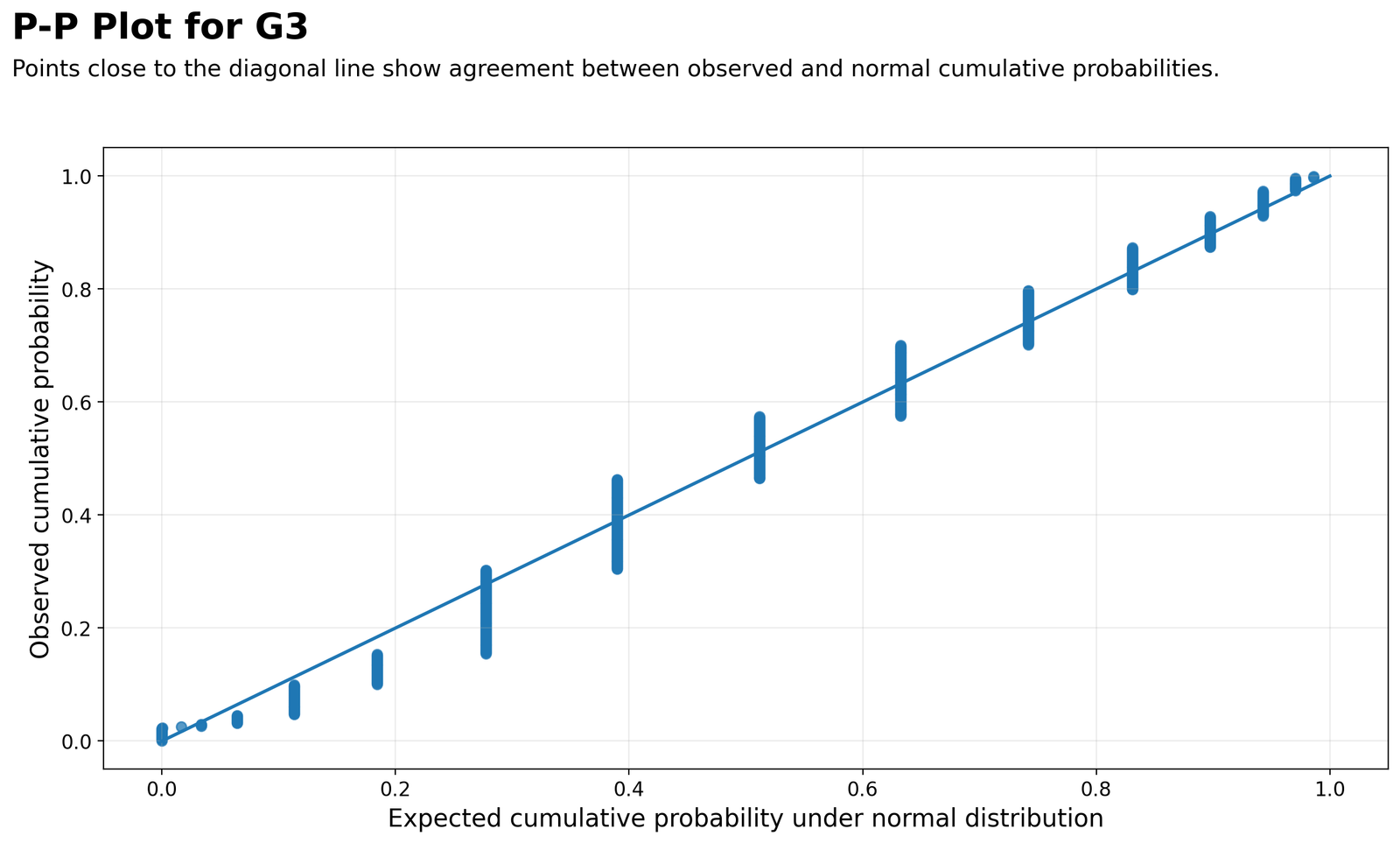
The P-P plot compares observed cumulative probabilities with expected cumulative probabilities under a normal distribution. Points close to the diagonal line suggest agreement between the observed and expected cumulative probabilities. In this chart, many points follow the diagonal reasonably well through the middle range, which means the cumulative pattern of G3 is not completely unrelated to a normal curve. However, the vertical step groups show that the variable has repeated integer scores, and several sections depart from the line. The lower-left region reflects the unusual low-score tail, while the middle probability bands show clustering around common grades such as 10, 11, 12 and 13. The P-P plot is often less sensitive to extreme tails than the Q-Q plot, so it may look more acceptable in the center. Even so, it still shows a distribution that is only approximately normal in the middle and not normal in the tails. For the hypothesis decision, the P-P plot supports the same conclusion: do not accept normality as a clean assumption for G3.
4. Standardized Normal Distribution for G3

This chart converts G3 scores into z-scores and compares the standardized values with the standard normal curve. In a standard normal distribution, the mean is 0 and the standard deviation is 1. SPSS confirms the standardized G3 z-score mean is approximately 0.0000 and the standard deviation is 1.0000. The dashed vertical guide lines show standard deviation positions. Most z-scores fall between about -1 and 1, which is expected for a central grade cluster. However, the left tail extends to about -3.69, while the right tail reaches only about 2.20. This imbalance is a strong visual sign of negative skewness. The very low G3 scores are much farther below the mean than the highest scores are above the mean. That is why the standardized chart does not match the standard normal curve perfectly. It supports rejecting the null hypothesis and helps explain the result in practical units: the problem is not just the center, but the unequal tail distance.
5. Empirical Rule Check
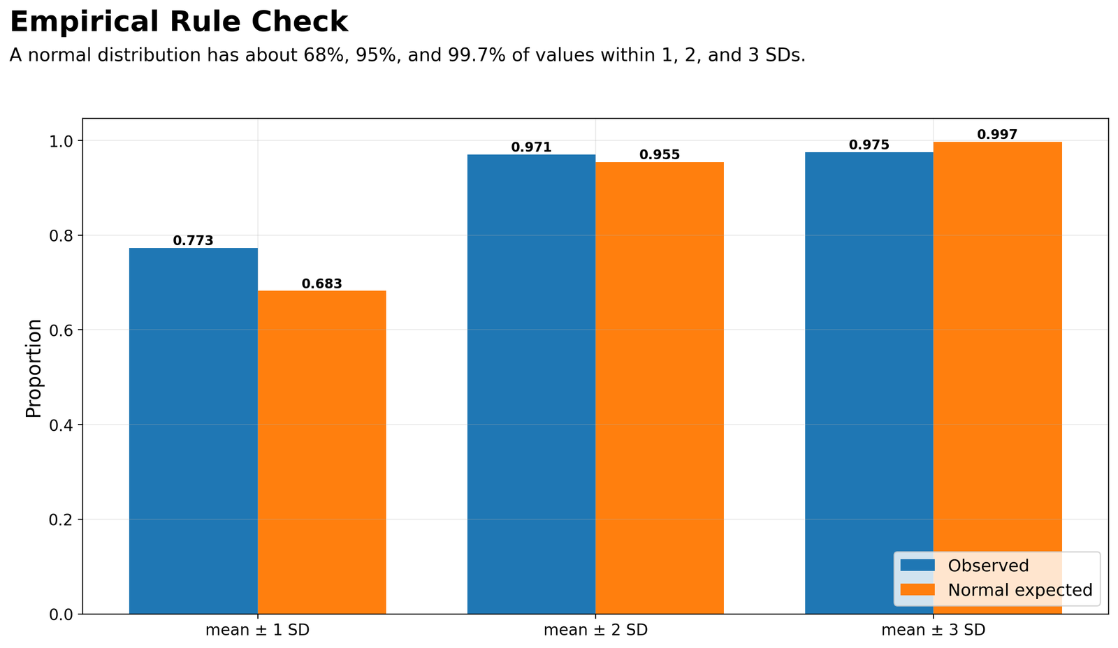
The empirical rule chart compares the observed G3 proportions with the expected proportions for a normal distribution. A normal distribution should place about 0.683 of values within one standard deviation, 0.955 within two standard deviations and 0.997 within three standard deviations. The observed G3 values are 0.773 within one standard deviation, 0.971 within two standard deviations and 0.975 within three standard deviations. The first result means G3 has more values packed near the center than a normal distribution would expect. The second result is also slightly higher than expected. The third result is lower than expected because 16 cases fall outside the three-standard-deviation band, mainly the very low grades. This is a strong practical explanation of the normality rejection: the center is crowded, but the extreme low tail is too far from the mean. Therefore, the empirical rule does not support a clean normal distribution.
R Validation Charts
The R charts validate the same result through a separate workflow. They confirm that the normality decision is not only a Python result. The R histogram, Q-Q plot, P-P plot, z-score chart and empirical rule chart all support the same interpretation: G3 has a central mound but does not fully satisfy normal distribution assumptions.
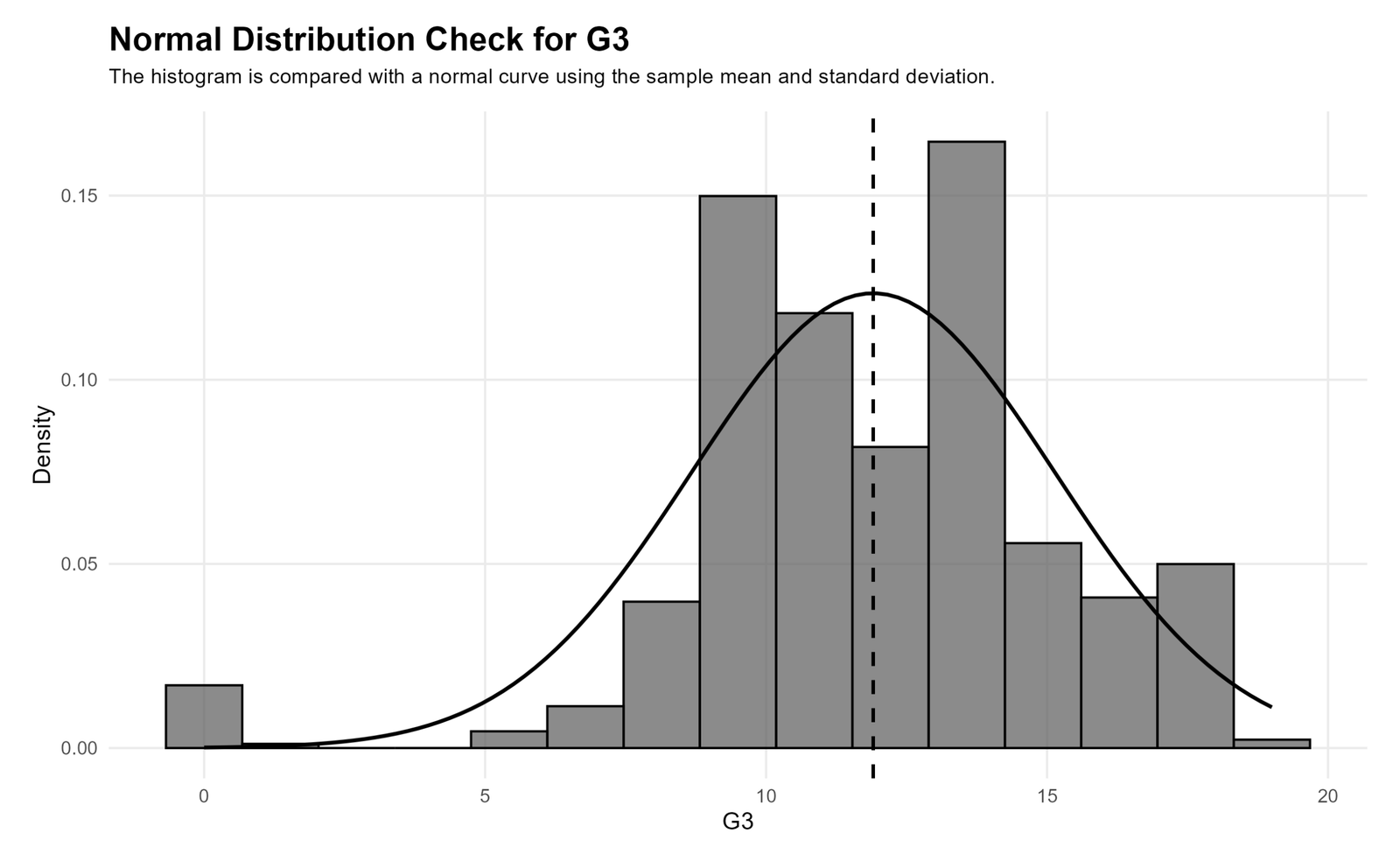
The R histogram confirms the same central pattern shown by Python. The G3 scores cluster in the middle, but the low-score tail and uneven bar heights prevent the distribution from matching a smooth bell curve. The fitted curve identifies where a normal distribution would place the density, while the observed bars show that the real data are more discrete and tail-heavy on the low side.
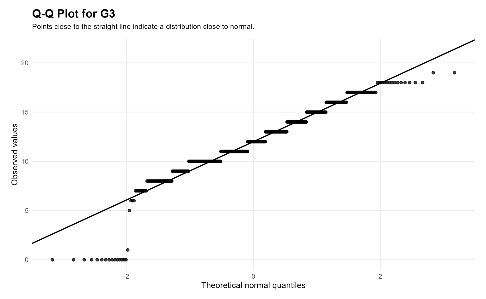
The R Q-Q plot again shows that the middle values follow the line better than the tails. The low scores depart strongly from the expected normal quantiles, and the upper scores flatten because G3 is bounded. This visual evidence supports the normality test decision to reject the null hypothesis.
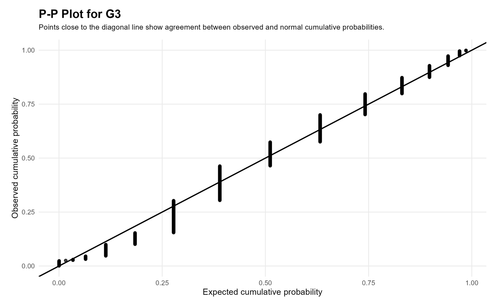
The R P-P plot shows cumulative probability agreement in some middle sections but visible step patterns and deviations across the range. Because G3 is an integer grade variable, repeated values create vertical clusters. The chart supports a moderate central fit but not a full normal distribution.

The R z-score chart confirms that standardizing G3 places the mean around 0 and the standard deviation around 1, but it also shows an unbalanced tail structure. The left tail reaches farther than the right tail, which matches the SPSS skewness value of -0.913. This confirms that the problem is not the scale of measurement; the problem is the shape of the distribution after standardization.
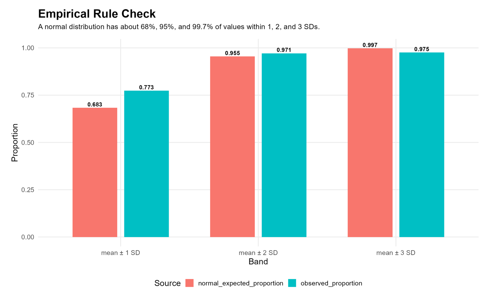
The R empirical rule chart validates the Python and SPSS proportions. The observed proportion within one standard deviation is higher than normal expectation, and the observed proportion within three standard deviations is lower than the 99.7% normal rule. This pattern indicates central clustering plus extreme low-tail influence. It supports the final conclusion that G3 is not normally distributed.
How to Check Normal Distribution in Python, R, SPSS and Excel
Normal Distribution Check in Python
Python can calculate descriptive statistics, z-scores, Q-Q plots, P-P plots, Shapiro-Wilk normality test and empirical rule checks.
import pandas as pd
import numpy as np
from scipy import stats
import matplotlib.pyplot as plt

df = pd.read_csv("spss_ready_data.csv")
g3 = pd.to_numeric(df["G3"], errors="coerce").dropna()

n = len(g3)
mean_g3 = g3.mean()
sd_g3 = g3.std(ddof=1)
z = (g3 - mean_g3) / sd_g3

print("H0: G3 is normally distributed.")
print("H1: G3 is not normally distributed.")
print("N:", n)
print("Mean:", round(mean_g3, 2))
print("SD:", round(sd_g3, 3))
print("Skewness:", round(stats.skew(g3, bias=False), 3))
print("Excess kurtosis:", round(stats.kurtosis(g3, fisher=True, bias=False), 3))

shapiro_stat, shapiro_p = stats.shapiro(g3)
print("Shapiro-Wilk:", round(shapiro_stat, 3), "p =", shapiro_p)

# Standard K-S using estimated mean and SD is not identical to SPSS Lilliefors correction.
ks_stat, ks_p = stats.kstest(g3, "norm", args=(mean_g3, sd_g3))
print("K-S:", round(ks_stat, 3), "p =", ks_p)

for k in [1, 2, 3]:
    observed = np.mean(np.abs(z) <= k)
    print(f"Within {k} SD:", round(observed, 3))

# Histogram with fitted normal curve
x = np.linspace(g3.min(), g3.max(), 300)
pdf = stats.norm.pdf(x, mean_g3, sd_g3)

plt.hist(g3, bins=15, density=True, alpha=0.65, edgecolor="black")
plt.plot(x, pdf, linewidth=3)
plt.axvline(mean_g3, linestyle="--", linewidth=2)
plt.title("Normal Distribution Check for G3")
plt.xlabel("G3")
plt.ylabel("Density")
plt.show()
Normal Distribution Check in R
R can calculate the same statistics and also run the Lilliefors test using the nortest package.
student <- read.csv("spss_ready_data.csv")
g3 <- na.omit(as.numeric(student$G3))

n_G3 <- length(g3)
mean_G3 <- mean(g3)
sd_G3 <- sd(g3)
z_G3 <- as.numeric(scale(g3))

cat("H0: G3 is normally distributed.\n")
cat("H1: G3 is not normally distributed.\n")
cat("N:", n_G3, "\n")
cat("Mean:", round(mean_G3, 2), "\n")
cat("SD:", round(sd_G3, 3), "\n")
cat("Minimum z:", round(min(z_G3), 2), "\n")
cat("Maximum z:", round(max(z_G3), 2), "\n")

shapiro.test(g3)

# install.packages("nortest")
library(nortest)
lillie.test(g3)

observed_1sd <- mean(abs(z_G3) <= 1)
observed_2sd <- mean(abs(z_G3) <= 2)
observed_3sd <- mean(abs(z_G3) <= 3)

print(data.frame(
  band = c("mean ± 1 SD", "mean ± 2 SD", "mean ± 3 SD"),
  observed = c(observed_1sd, observed_2sd, observed_3sd),
  normal_expected = c(0.683, 0.955, 0.997)
))
Normal Distribution Check in SPSS
SPSS can produce descriptives, normality tests, histograms, Q-Q plots, detrended Q-Q plots and z-score variables.
* Normal Distribution Analysis for G3 Final Grade.
* H0: G3 is normally distributed.
* H1: G3 is not normally distributed.

SET UNICODE=ON.
SET DECIMAL=DOT.
SET PRINTBACK=OFF.
SET MPRINT=OFF.

GET DATA
 /TYPE=TXT
 /FILE="D:\DATA ANALYSIS\B Normality and Assumption Tests\Normal Distribution\SPSS_Output\clean_data\spss_ready_data.csv"
 /ENCODING='UTF8'
 /DELCASE=LINE
 /DELIMITERS=","
 /QUALIFIER='"'
 /ARRANGEMENT=DELIMITED
 /FIRSTCASE=2
 /IMPORTCASE=ALL.

DATASET NAME StudentData WINDOW=FRONT.

TITLE "Normal Distribution Analysis for G3 Final Grade".

DESCRIPTIVES VARIABLES=G3
 /SAVE
 /STATISTICS=MEAN STDDEV MIN MAX.

FREQUENCIES VARIABLES=G3 ZG3
 /STATISTICS=MEAN MEDIAN MODE STDDEV VARIANCE SKEWNESS SESKEW KURTOSIS SEKURT RANGE MINIMUM MAXIMUM
 /ORDER=ANALYSIS.

EXAMINE VARIABLES=G3
 /PLOT BOXPLOT HISTOGRAM NPPLOT
 /STATISTICS DESCRIPTIVES
 /CINTERVAL 95
 /MISSING LISTWISE
 /NOTOTAL.

NPAR TESTS
 /K-S(NORMAL)=G3
 /MISSING ANALYSIS.

COMPUTE within_1sd = (ABS(ZG3) <= 1).
COMPUTE within_2sd = (ABS(ZG3) <= 2).
COMPUTE within_3sd = (ABS(ZG3) <= 3).
EXECUTE.

FREQUENCIES VARIABLES=within_1sd within_2sd within_3sd.

OUTPUT EXPORT
 /CONTENTS EXPORT=VISIBLE
 /PDF DOCUMENTFILE="D:\DATA ANALYSIS\B Normality and Assumption Tests\Normal Distribution\SPSS_Output\Normal-Distribution-SPSS-Output.pdf".
Normal Distribution Check in Excel
Excel can calculate a normal distribution curve, z-scores and empirical rule counts. If G3 values are in B2:B650, use these formulas.
| Excel task | Formula | Purpose |
|---|---|---|
| Mean | =AVERAGE(B2:B650) | Calculates the center of G3. |
| Standard deviation | =STDEV.S(B2:B650) | Calculates the sample spread. |
| Skewness | =SKEW(B2:B650) | Checks left or right asymmetry. |
| Kurtosis | =KURT(B2:B650) | Checks excess tail weight. |
| Z-score for row 2 | =(B2-$E$2)/$E$3 | Assumes mean is in E2 and SD is in E3. |
| Normal density | =NORM.DIST(B2,$E$2,$E$3,FALSE) | Creates fitted normal curve values. |
| Normal cumulative probability | =NORM.DIST(B2,$E$2,$E$3,TRUE) | Creates expected cumulative probabilities. |
| Within 1 SD | =COUNTIFS(C2:C650,">=-1",C2:C650,"<=1")/COUNT(C2:C650) | Checks observed proportion within one standard deviation. |
| Within 2 SD | =COUNTIFS(C2:C650,">=-2",C2:C650,"<=2")/COUNT(C2:C650) | Checks observed proportion within two standard deviations. |
| Within 3 SD | =COUNTIFS(C2:C650,">=-3",C2:C650,"<=3")/COUNT(C2:C650) | Checks observed proportion within three standard deviations. |
How to Report the Normal Distribution Decision
A good normal distribution report should include the variable, sample size, mean, standard deviation, skewness, kurtosis, normality test results, p-value decision and visual interpretation. It should also mention whether the null hypothesis was rejected or not.
APA-style report: Normality was assessed for G3 final grade using visual plots and formal normality tests. The variable had 649 valid observations, with M = 11.91 and SD = 3.231. The distribution showed negative skewness (skewness = -0.913) and positive kurtosis (kurtosis = 2.712). The Kolmogorov-Smirnov test with Lilliefors correction was significant, D(649) = .124, p < .001, and the Shapiro-Wilk test was also significant, W(649) = .926, p < .001. Therefore, the null hypothesis of normality was rejected. The histogram, Q-Q plot, P-P plot and z-score distribution confirmed that G3 had a central mound but deviated from normality because of a low-score tail.
Plain-language report: G3 final grade is not normally distributed. Most scores are near the middle, around 10 to 15, but several very low scores create a left-tail problem. The normality tests were significant, so the normal distribution assumption should not be accepted without caution.
When normality is rejected, the next decision depends on the purpose of the analysis. Some methods are robust when sample size is large, especially if group sizes are reasonable. However, for assumption-heavy analysis, check transformations, robust methods, nonparametric alternatives or residual-based diagnostics. For possible transformation workflows, see reciprocal transformation. For variance assumptions, use Levene test, Brown-Forsythe test or Cochran C test. For regression assumption diagnostics, see Ramsey RESET test and Goldfeld-Quandt test.
Common Mistakes
1. Saying p = .000 means the p-value is zero
SPSS displays .000 when the value is very small. In reporting, write p < .001.
2. Accepting normality because the histogram looks roughly bell-shaped
The histogram may look approximately bell-shaped in the middle, but the tails can still violate normality. For G3, the low-score tail is the main issue.
3. Ignoring the Q-Q plot tails
The center of a Q-Q plot can look acceptable while the tails show strong departures. Normality requires the whole distribution to behave reasonably, not only the middle.
4. Confusing normal distribution with standard normal distribution
A normal distribution can have any mean and standard deviation. A standard normal distribution always has mean 0 and standard deviation 1.
5. Treating large-sample normality tests too mechanically
Large samples can make small deviations statistically significant. Use visual evidence, sample size and analysis purpose together.
6. Forgetting that grade data are discrete
G3 is an integer grade variable, so Q-Q and P-P plots show step patterns. This discreteness contributes to departures from a smooth continuous normal curve.
7. Not linking normality to the planned analysis
Normality is not checked for its own sake. It should be connected to the next method, such as a t test, ANOVA, regression model, confidence interval or transformation decision.
Download SPSS Output and Verification Files
The SPSS output PDF verifies the descriptive statistics, G3 frequency table, z-score table, Kolmogorov-Smirnov test, Shapiro-Wilk test, normal curve histogram, Q-Q plot, detrended Q-Q plot and empirical rule counts used in this guide.
External References for Normal Distribution
This post uses verified Python, R and SPSS outputs together with standard statistical documentation and dataset references.
FAQs About Normal Distribution
What is normal distribution?
Normal distribution is a bell-shaped probability distribution where values are symmetrically distributed around the mean.
What is the normal distribution formula?
The normal distribution formula is f(x) = [1 / (σ√(2π))] × e^[-(x - μ)² / (2σ²)], where μ is the mean and σ is the standard deviation.
What is the standard normal distribution?
The standard normal distribution is a normal distribution with mean 0 and standard deviation 1.
What is the null hypothesis for a normality test?
The null hypothesis is that the variable follows a normal distribution.
What is the alternative hypothesis for a normality test?
The alternative hypothesis is that the variable does not follow a normal distribution.
Was G3 normally distributed?
No. The Kolmogorov-Smirnov and Shapiro-Wilk tests were significant with p < .001, so the null hypothesis of normality was rejected.
What were the SPSS normality test results for G3?
The Kolmogorov-Smirnov statistic was .124 with df = 649 and p < .001. The Shapiro-Wilk statistic was .926 with df = 649 and p < .001.
What does the Q-Q plot show?
The Q-Q plot shows whether observed values follow theoretical normal quantiles. For G3, the middle values were closer to the line, but the tails deviated, especially the low-score tail.
What does the P-P plot show?
The P-P plot compares observed and expected cumulative probabilities. For G3, it showed partial agreement in the middle but visible departures and step patterns.
What is the empirical rule?
The empirical rule says a normal distribution has about 68.3% of values within one standard deviation, 95.5% within two standard deviations and 99.7% within three standard deviations.
What were the empirical rule results for G3?
G3 had 77.3% of values within one standard deviation, 97.1% within two standard deviations and 97.5% within three standard deviations.
How do you check normal distribution in Excel?
Calculate the mean, standard deviation and z-scores, then use NORM.DIST for the expected normal curve and compare observed values with expected proportions.

