
Z-Scores, Normal Curve, Empirical Rule and Normality Diagnostics
Standard Normal Distribution: Formula, Z-Score, Interpretation, SPSS, Python, R and Excel Guide
Standard Normal Distribution is the normal distribution after standardization, where the mean becomes 0 and the standard deviation becomes 1. It is used to interpret z-scores, compare values measured on different scales, calculate probabilities, apply the empirical rule, and check normality. This guide explains Standard Normal Distribution with verified SPSS output, Python charts, R validation charts, Excel workflow, z-score formula, Q-Q plot, empirical CDF, normality tests, APA reporting wording, and downloadable resources.
Quick Answer: Standard Normal Distribution Result
The verified SPSS output standardizes G3 final grade into a z-score variable. The original G3 variable has N = 649, minimum = 0, maximum = 19, mean = 11.91, and standard deviation = 3.231. After z-score transformation, the standardized G3 variable has N = 649, minimum z = -3.685, maximum z = 2.196, mean = .00000, and standard deviation = 1.000000. This confirms that the z-score transformation worked correctly.
Hypothesis-style interpretation: A perfect standard normal variable has mean = 0, standard deviation = 1, skewness = 0, and kurtosis = 0 when excess kurtosis is used. The standardized G3 variable has the expected mean and standard deviation, but its shape is not perfectly normal. SPSS reports skewness = -0.913, kurtosis = 2.712, Kolmogorov-Smirnov D = .124, p < .001, and Shapiro-Wilk W = .926, p < .001. Therefore, the variable is correctly standardized, but it does not perfectly follow a normal distribution.
Final interpretation: The z-score transformation successfully converted G3 into a standardized variable with mean approximately 0 and standard deviation 1. However, the normality output shows that the standardized scores are not perfectly normal because the distribution is negatively skewed and leptokurtic. The Standard Normal Distribution framework is still useful for interpreting relative standing, z-score bands, empirical rule comparisons, and normality diagnostics.
Important note: Standardizing a variable does not automatically make it normally distributed. A z-score transformation changes the scale to mean 0 and standard deviation 1, but it does not remove skewness, kurtosis, outliers, or distributional irregularities. This is why the Q-Q plot, empirical CDF, Kolmogorov-Smirnov test, and Shapiro-Wilk test are still needed.
Table of Contents
- What Is the Standard Normal Distribution?
- Standard Normal Distribution Formula and Z-Score Formula
- Null and Alternative Hypothesis for Standard Normal Distribution
- Dataset and Standardized Variables Used
- Verified SPSS Output Interpretation
- Python Chart-by-Chart Interpretation
- R Chart-by-Chart Validation
- SPSS, R, Python and Excel Workflows
- Code Blocks for Standard Normal Distribution
- APA Reporting Wording
- Common Mistakes
- When to Use Standard Normal Distribution
- Downloads and Resources
- Related Guides
- FAQs
What Is the Standard Normal Distribution?
The Standard Normal Distribution is a special normal distribution with a mean of 0 and a standard deviation of 1. Values on this distribution are called z-scores. A z-score tells how many standard deviations a value is above or below the mean. A z-score of 0 means the value is exactly at the mean. A z-score of +1 means the value is one standard deviation above the mean. A z-score of -1 means the value is one standard deviation below the mean.
The Standard Normal Distribution is useful because it allows scores measured on different scales to be compared on the same standardized scale. For example, a final grade, an age value, and an absence count are measured differently, but after standardization, each value can be interpreted as a z-score. This makes the Standard Normal Distribution important for probability, confidence intervals, normality checks, regression diagnostics, outlier detection, and hypothesis testing.
In this guide, the main variable is G3 final grade. SPSS first reports the original G3 mean and standard deviation. Then it reports the standardized G3 z-score variable. The standardized variable has mean .00000 and standard deviation 1.000000, confirming a correct z-score transformation. However, the distribution shape is not perfectly normal because skewness, kurtosis, and normality tests show departures from the theoretical normal curve.
Practical meaning: The Standard Normal Distribution does not mean every dataset is normal. It gives a reference curve. A standardized variable has mean 0 and standard deviation 1, but it may still have skewness, kurtosis, heavy tails, outliers, or non-normal shape.
Standard Normal Distribution Formula and Z-Score Formula
The Standard Normal Distribution is commonly written as:
This means the standardized variable Z follows a normal distribution with mean 0 and variance 1. The standard deviation is also 1 because the square root of variance 1 is 1.
The z-score formula is:
When working with sample data, the sample version is usually written as:
For the G3 example, the sample mean is 11.91 and the sample standard deviation is 3.231. Therefore, a student with G3 = 15 would have an approximate z-score of:
This means a G3 score of 15 is about 0.96 standard deviations above the mean. A G3 score of 0 has a z-score near -3.685, which means it is far below the mean and contributes strongly to the lower tail of the standardized distribution.
| Z-score | Position | Simple Meaning | G3 Example Interpretation |
|---|---|---|---|
| z = 0 | At the mean | Average score | G3 is near 11.91. |
| z = +1 | One SD above mean | Above average | G3 is about 15.14. |
| z = -1 | One SD below mean | Below average | G3 is about 8.68. |
| z = +2 | Two SD above mean | High score region | G3 is about 18.37. |
| z = -2 | Two SD below mean | Low score region | G3 is about 5.45. |
| z = -3.685 | Extreme low tail | Very far below mean | Observed minimum G3 = 0. |
Null and Alternative Hypothesis for Standard Normal Distribution
The Standard Normal Distribution itself is a theoretical reference distribution. In applied data analysis, the hypothesis question is usually whether a standardized variable is consistent with a normal distribution. Because z-standardization always forces mean near 0 and standard deviation near 1, the real diagnostic question is about distribution shape.
| Statement | Hypothesis | Meaning in This Example |
|---|---|---|
| Standardization check | z mean ≈ 0 and z SD ≈ 1 | The G3 z-score transformation worked correctly. |
| Normality null hypothesis | H0: z-scores follow a normal distribution | The standardized G3 distribution matches the theoretical normal curve. |
| Normality alternative hypothesis | H1: z-scores do not follow a normal distribution | The standardized G3 distribution departs from the theoretical normal curve. |
| Decision rule | Reject H0 if p < .05 | Both Kolmogorov-Smirnov and Shapiro-Wilk are significant. |
Hypothesis-style decision: The z-score transformation is correct because the standardized G3 variable has mean approximately 0 and standard deviation 1. However, the normality tests are significant: Kolmogorov-Smirnov D = .124, p < .001 and Shapiro-Wilk W = .926, p < .001. Therefore, the standardized G3 scores are not perfectly normally distributed.
Interpretation nuance: A significant normality test does not mean z-scores were calculated incorrectly. It means the original distribution shape remains non-normal after standardization. Standardization changes location and scale, not shape.
Dataset and Standardized Variables Used
The worked example uses the student performance data structure. The main standardized variable is G3 final grade. The SPSS output also lists key numeric measures: G1, G2, G3, age, and absences. The purpose is to show how a raw variable can be converted into a z-score variable and then compared with the Standard Normal Distribution.
| Variable | Role | N | Mean | Standard Deviation | Why It Matters |
|---|---|---|---|---|---|
| G1 | Key measure | 649 | 11.40 | 2.745 | First-period grade, useful for comparison with later grade variables. |
| G2 | Key measure | 649 | 11.57 | 2.914 | Second-period grade, often strongly related to G3. |
| G3 | Main variable | 649 | 11.91 | 3.231 | Final grade converted into a standard normal z-score variable. |
| Age | Key measure | 649 | 16.74 | 1.218 | Age variable used as an additional descriptive measure. |
| Absences | Key measure | 649 | 3.66 | 4.641 | Count variable with wider spread and a different scale. |
Before standardizing a variable, it is useful to review descriptive statistics, frequency distribution, histogram interpretation, box plot interpretation, and five-number summary.
Verified SPSS Output Interpretation
The SPSS output verifies the standardization and normality interpretation. It shows the original G3 descriptive statistics, the standardized G3 z-score statistics, z-score bands, histogram/Q-Q plot output, normality tests, skewness, kurtosis, and descriptive statistics for key numeric variables.
SPSS Descriptive Output for Original G3 and Standardized G3
| SPSS Output Item | Original G3 | Standardized G3 z-score | Interpretation |
|---|---|---|---|
| N | 649 | 649 | All valid cases were standardized. |
| Minimum | 0 | -3.685 | The lowest G3 score is 3.685 standard deviations below the mean. |
| Maximum | 19 | 2.196 | The highest G3 score is 2.196 standard deviations above the mean. |
| Mean | 11.91 | .00000 | The z-score mean is correctly centered at zero. |
| Standard deviation | 3.231 | 1.000000 | The z-score standard deviation is correctly scaled to one. |
SPSS z-Score Band Frequencies
| Z-score band label | Frequency | Percent | Cumulative Percent | Interpretation |
|---|---|---|---|---|
| -4.00 | 16 | 2.5% | 2.5% | Very low z-score region. |
| -3.00 | 1 | 0.2% | 2.6% | Low extreme band. |
| -2.00 | 48 | 7.4% | 10.0% | Below-average band. |
| -1.00 | 236 | 36.4% | 46.4% | Lower central band. |
| 1.00 | 266 | 41.0% | 87.4% | Upper central band. |
| 2.00 | 80 | 12.3% | 99.7% | Upper above-average band. |
| 3.00 | 2 | 0.3% | 100.0% | High z-score band. |
SPSS Normality Output for Standardized G3
| Statistic | SPSS Value | Interpretation |
|---|---|---|
| Mean | .00000 | The standardized mean is centered at zero. |
| 95% CI for mean | -.07708 to .07708 | The standardized mean is very close to zero. |
| 5% trimmed mean | .04687 | The trimmed mean shifts slightly upward because low scores affect the raw mean. |
| Median | .02909 | The median is close to zero but slightly above it. |
| Variance | 1.000 | The z-score variance is one. |
| Standard deviation | 1.000000 | The z-score standard deviation is one. |
| Minimum | -3.685 | Some values are far below the mean. |
| Maximum | 2.196 | The upper tail is less extreme than the lower tail. |
| Range | 5.881 | The z-score spread covers nearly six standard-deviation units. |
| Interquartile range | 1.238 | The middle 50% of standardized values spans 1.238 z units. |
| Skewness | -.913 | The standardized G3 distribution is negatively skewed. |
| Kurtosis | 2.712 | The distribution is more peaked/heavy-tailed than a normal distribution. |
| Kolmogorov-Smirnov | D = .124, p < .001 | Reject normality under the K-S test. |
| Shapiro-Wilk | W = .926, p < .001 | Reject normality under the Shapiro-Wilk test. |
SPSS interpretation summary: Standardization was successful because the z-score variable has mean 0 and standard deviation 1. However, the standardized G3 distribution is not perfectly normal because skewness is negative, kurtosis is positive, and both normality tests are significant at p < .001.
Python Chart-by-Chart Interpretation
The Python charts show how the standardized G3 variable behaves against the Standard Normal Distribution. The chart set includes the z-score distribution with normal curve, Standard Normal Q-Q plot, empirical CDF versus normal CDF, z-score band percentages, and empirical rule comparison.
Python Chart 1: Z Distribution with Normal Curve
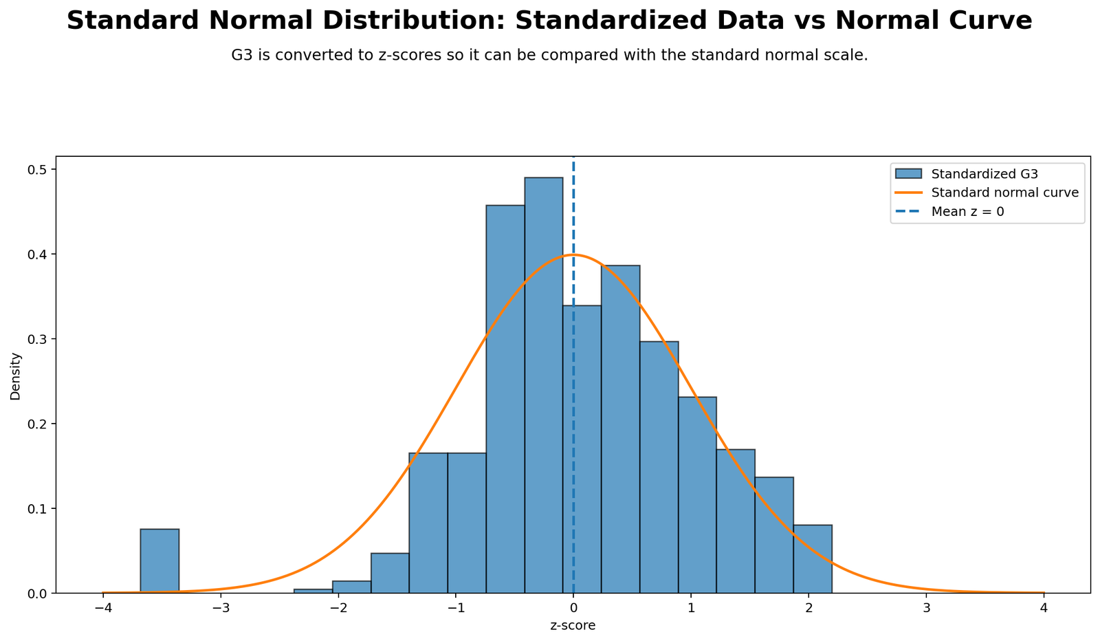
This chart shows the distribution of standardized G3 z-scores against the theoretical Standard Normal curve. The z-score scale places the mean near 0 and the standard deviation near 1. The curve provides the normal reference shape, while the histogram shows the actual standardized G3 data. The important point is that the transformation has centered and scaled the variable correctly, but the bars do not perfectly match the theoretical curve.
The left tail extends farther than the right tail because the minimum z-score is -3.685, while the maximum is 2.196. This asymmetry matches the SPSS skewness value of -0.913. Therefore, the chart supports two conclusions: first, standardization worked; second, the standardized distribution is not perfectly normal in shape.
Python Chart 2: Standard Normal Q-Q Plot
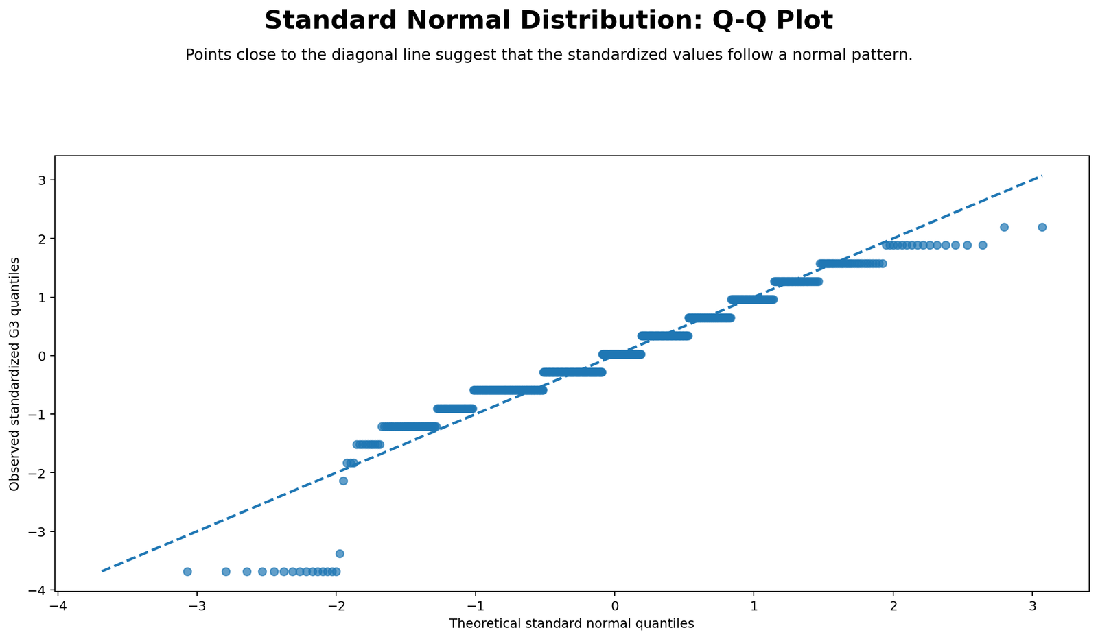
The Q-Q plot checks whether the standardized G3 values follow the theoretical normal line. If the data were perfectly normal, the points would fall close to the diagonal line from the lower tail to the upper tail. In this example, the central values are closer to the reference line, but tail values depart from the line. The strongest departure is expected in the lower tail because some G3 values are far below the mean.
This chart confirms the SPSS normality tests. The z-score variable has the correct mean and standard deviation, but the Q-Q pattern indicates tail departures from normality. For a full normality workflow, this chart should be interpreted alongside the Q-Q plot normality check, Kolmogorov-Smirnov test, and Lilliefors test.
Python Chart 3: Empirical CDF vs Normal CDF
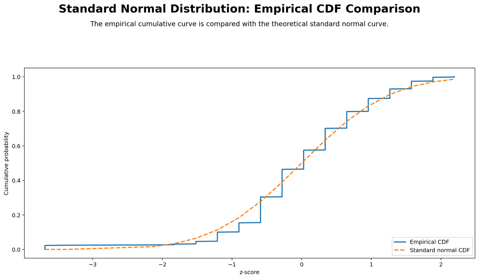
This chart compares the empirical cumulative distribution function with the theoretical normal CDF. The empirical CDF shows the actual cumulative percentage of standardized G3 scores at each z-score level. The normal CDF shows what those cumulative percentages would look like under a perfect Standard Normal Distribution.
Where the two curves overlap, the standardized data behave similarly to the normal reference. Where they separate, the actual distribution differs from normal. This chart is especially helpful because it shows cumulative differences across the entire z-score scale, not just the center or the tails. The observed departures support the SPSS decision that the standardized G3 distribution is not perfectly normal.
Python Chart 4: Z-Score Band Percentages

This chart summarizes how standardized G3 values are distributed across z-score bands. The SPSS frequency output shows that the two central bands labeled -1.00 and 1.00 contain the largest percentages, with 36.4% and 41.0% respectively. Together, these central bands contain most of the observations. This supports the practical idea that many students are near the mean.
The lower-tail bands also matter. The minimum standardized value is -3.685, meaning a small number of observations fall far below the mean. These low values create negative skewness and contribute to the normality-test rejection. Therefore, the z-score band chart is useful for explaining where the distribution differs from the theoretical Standard Normal Distribution.
Python Chart 5: Empirical Rule Comparison
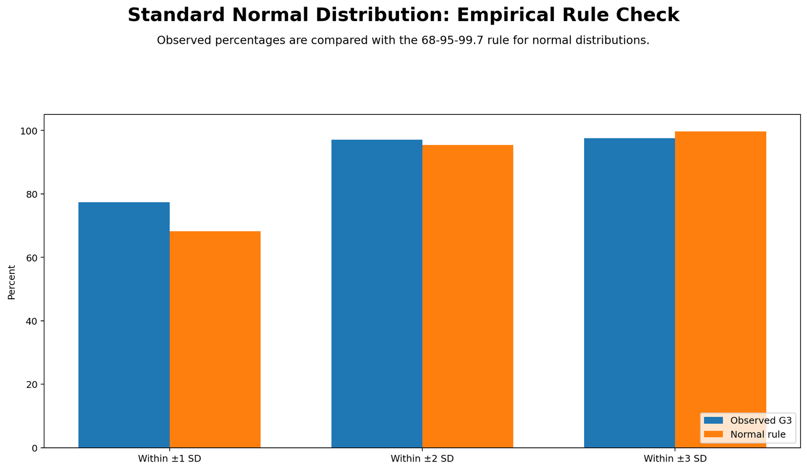
The empirical rule says that, in a perfect normal distribution, about 68% of values fall within ±1 standard deviation, about 95% fall within ±2 standard deviations, and about 99.7% fall within ±3 standard deviations. This chart compares those theoretical expectations with the observed standardized G3 distribution.
The empirical rule comparison helps readers understand whether the standardized variable behaves like a normal variable in practical terms. If the observed percentages are close to 68%, 95%, and 99.7%, the distribution is approximately normal. If the observed percentages differ, the chart helps identify the practical size of the departure. In this example, the normality tests and tail behavior show that the standardized G3 distribution is not perfectly normal, even though it is correctly centered and scaled.
R Chart-by-Chart Validation
The R charts validate the same Standard Normal Distribution workflow using a separate software environment. The R figures confirm the z-score distribution, Q-Q plot pattern, empirical CDF comparison, z-score bands, and empirical rule comparison.
R Chart 1: Z Distribution with Normal Curve
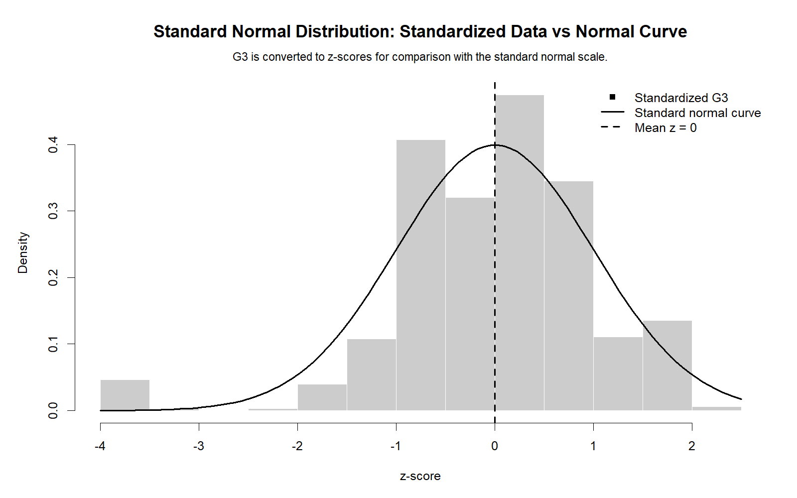
The R distribution chart confirms that the z-score transformation centers the distribution around 0 and scales it to standard deviation 1. It also confirms that the actual standardized G3 distribution does not perfectly match the theoretical normal curve. The same left-tail behavior remains visible.
R Chart 2: Standard Normal Q-Q Plot
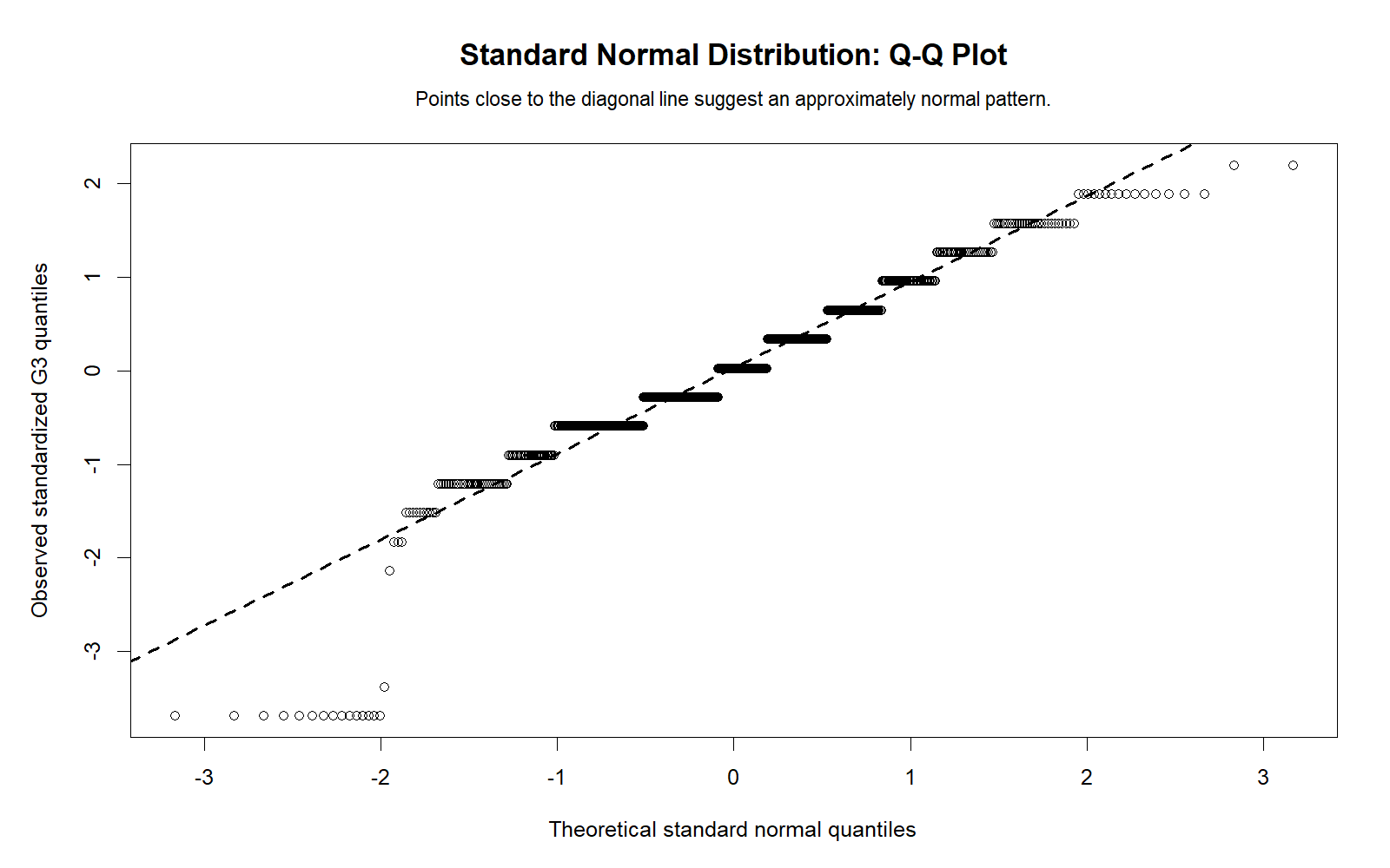
The R Q-Q plot validates the Python Q-Q interpretation. Central values generally follow the reference line more closely than tail values. Tail departures show that the standardized G3 scores are not perfectly normal. This agrees with the SPSS Kolmogorov-Smirnov and Shapiro-Wilk tests.
R Chart 3: Empirical CDF vs Normal CDF
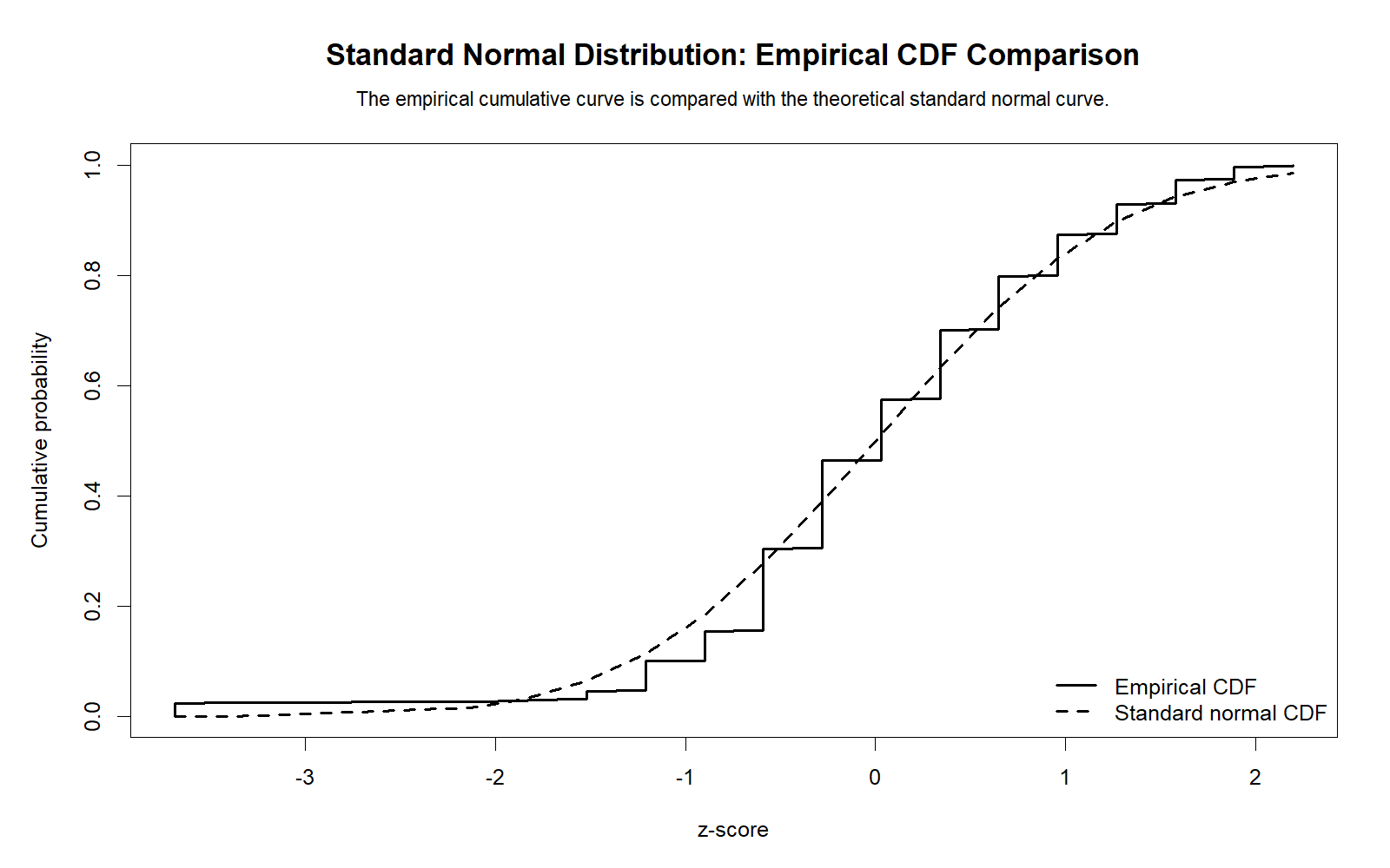
The R empirical CDF chart confirms the same cumulative-distribution pattern. The empirical curve follows the normal CDF in some regions but differs in others. This validates the conclusion that the standardized G3 variable is useful for z-score interpretation but not perfectly normal in distribution shape.
R Chart 4: Z-Score Band Percentages

The R z-score band chart confirms the band interpretation from Python and SPSS. Most values are in the central z-score bands, while smaller percentages appear in the extreme bands. The lower-tail bands are important because they explain the negative skewness and the non-normality decision.
R Chart 5: Empirical Rule Comparison
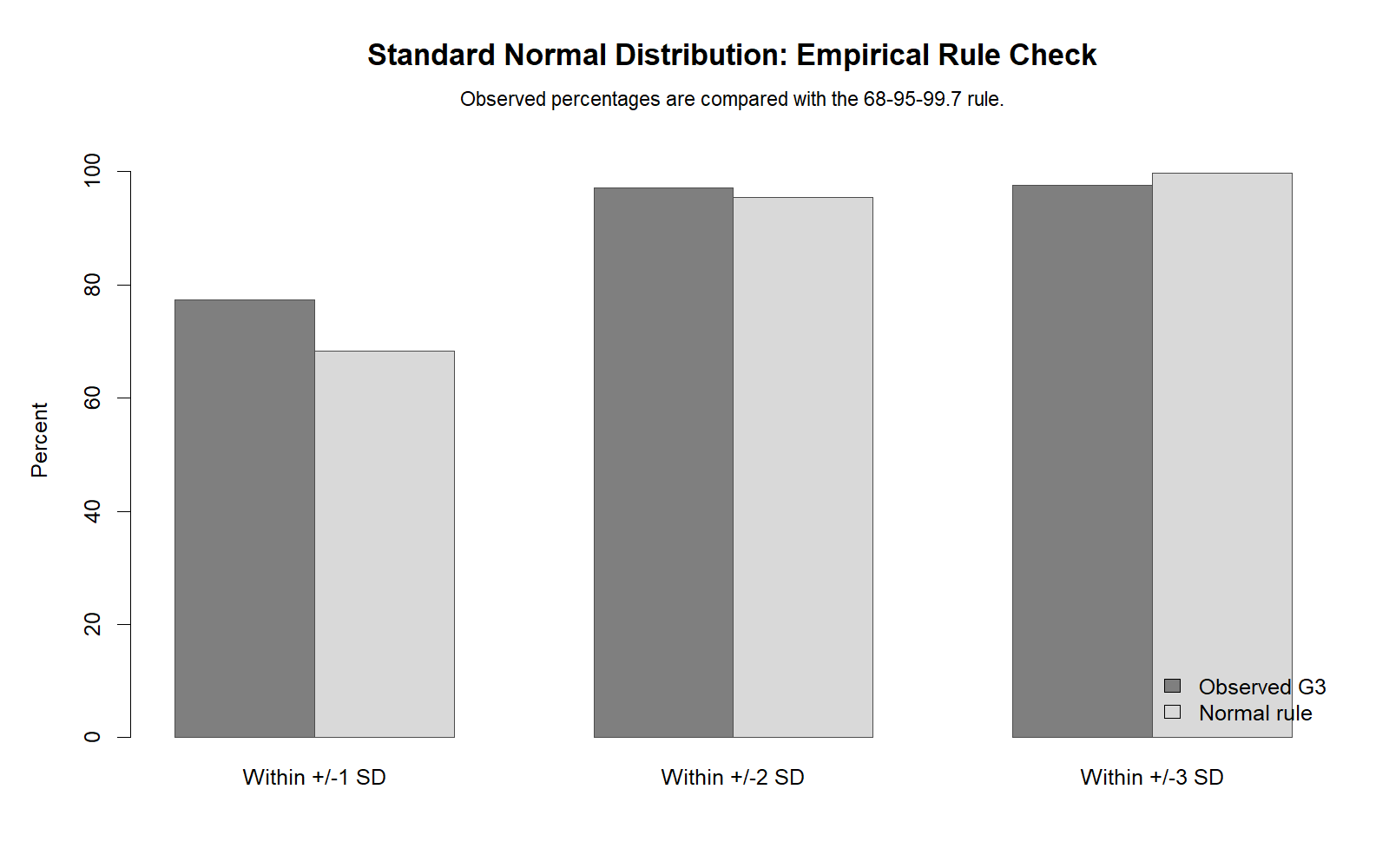
The R empirical rule chart confirms whether the standardized G3 distribution approximates the expected normal percentages within ±1, ±2, and ±3 standard deviations. It validates the Python chart and helps readers see the practical difference between standardization and true normality. The variable is standardized correctly, but its shape still departs from the normal reference.
SPSS, R, Python and Excel Workflows for Standard Normal Distribution
The same Standard Normal Distribution workflow can be reproduced in SPSS, R, Python and Excel. The key steps are to calculate the mean, calculate the standard deviation, compute z-scores, check the z-score mean and standard deviation, and then compare the standardized distribution against the theoretical normal distribution.
SPSS Workflow
| Step | SPSS Menu or Syntax | Purpose |
|---|---|---|
| Open dataset | File > Open > Data | Load the SPSS-ready dataset. |
| Run descriptives | Analyze > Descriptive Statistics > Descriptives | Get mean and standard deviation for G3. |
| Save standardized value | Descriptives > Save standardized values as variables | Create a z-score variable for G3. |
| Check z summary | Descriptives on z-score variable | Confirm mean = 0 and SD = 1. |
| Run Explore | Analyze > Descriptive Statistics > Explore | Get histogram, Q-Q plot, skewness, kurtosis and normality tests. |
| Export output | File > Export or OUTPUT EXPORT | Save SPSS output PDF. |
R Workflow
| Step | R Action | Purpose |
|---|---|---|
| Read data | read.csv() | Load the dataset. |
| Calculate z-score | scale(G3) | Standardize G3 to mean 0 and SD 1. |
| Check summary | mean(), sd() | Verify z mean and z standard deviation. |
| Make Q-Q plot | qqnorm(), qqline() | Check normality visually. |
| Compare CDF | ecdf(), pnorm() | Compare empirical and theoretical cumulative probabilities. |
| Build charts | Base R or ggplot2 | Create WordPress-ready visuals. |
Python Workflow
| Step | Python Action | Purpose |
|---|---|---|
| Read data | pandas.read_csv() | Load the dataset into a DataFrame. |
| Calculate z-score | scipy.stats.zscore() or manual formula | Create standardized values. |
| Check summary | mean(), std() | Verify mean ≈ 0 and SD ≈ 1. |
| Make Q-Q plot | scipy.stats.probplot() | Compare observed quantiles with normal quantiles. |
| Compare CDF | stats.norm.cdf() | Compare empirical CDF with normal CDF. |
| Create plots | matplotlib | Generate hosted chart images. |
Excel Workflow
| Excel Task | Formula or Tool | Purpose |
|---|---|---|
| Mean | =AVERAGE(A2:A650) | Calculate the raw G3 mean. |
| Standard deviation | =STDEV.S(A2:A650) | Calculate sample standard deviation. |
| Z-score | =(A2-$B$1)/$B$2 | Standardize each value using mean in B1 and SD in B2. |
| Normal CDF | =NORM.S.DIST(z,TRUE) | Calculate cumulative probability for a z-score. |
| Normal density | =NORM.S.DIST(z,FALSE) | Calculate the standard normal curve height. |
| Empirical rule check | =COUNTIFS(z_range,">=-1",z_range,"<=1")/COUNT(z_range) | Find the observed percentage within ±1 SD. |
Code Blocks for Standard Normal Distribution
SPSS Syntax for Standard Normal Distribution
* Standard Normal Distribution and z-score workflow in SPSS.
* Main variable: G3 final grade.

TITLE "Standard Normal Distribution: G3 z-score transformation".

DESCRIPTIVES VARIABLES=G3
  /SAVE
  /STATISTICS=MEAN STDDEV MIN MAX.

* SPSS creates standardized variable automatically, usually named ZG3.
DESCRIPTIVES VARIABLES=G3 ZG3
  /STATISTICS=MEAN STDDEV MIN MAX.

FREQUENCIES VARIABLES=ZG3
  /FORMAT=NOTABLE
  /STATISTICS=MEAN MEDIAN STDDEV VARIANCE SKEWNESS KURTOSIS MINIMUM MAXIMUM
  /HISTOGRAM NORMAL.

EXAMINE VARIABLES=ZG3
  /PLOT BOXPLOT HISTOGRAM NPPLOT
  /COMPARE GROUPS
  /STATISTICS DESCRIPTIVES
  /CINTERVAL 95
  /MISSING LISTWISE
  /NOTOTAL.

OUTPUT EXPORT
  /CONTENTS EXPORT=VISIBLE
  /PDF DOCUMENTFILE="Standard-Normal-Distribution-SPSS-Output.pdf".
Python Code for Standard Normal Distribution
import pandas as pd
import numpy as np
from scipy import stats

df = pd.read_csv("dataset.csv")

x = pd.to_numeric(df["G3"], errors="coerce").dropna()

mean_x = x.mean()
sd_x = x.std(ddof=1)

z = (x - mean_x) / sd_x

print("Original G3 mean:", mean_x)
print("Original G3 SD:", sd_x)
print("Z mean:", z.mean())
print("Z SD:", z.std(ddof=1))
print("Z min:", z.min())
print("Z max:", z.max())

# Normality tests
ks_stat, ks_p = stats.kstest(z, "norm")
shapiro_stat, shapiro_p = stats.shapiro(z)

print("Kolmogorov-Smirnov statistic:", ks_stat)
print("Kolmogorov-Smirnov p:", ks_p)
print("Shapiro-Wilk statistic:", shapiro_stat)
print("Shapiro-Wilk p:", shapiro_p)

# Empirical rule percentages
within_1 = np.mean((z >= -1) & (z <= 1)) * 100
within_2 = np.mean((z >= -2) & (z <= 2)) * 100
within_3 = np.mean((z >= -3) & (z <= 3)) * 100

print("Within ±1 SD:", within_1)
print("Within ±2 SD:", within_2)
print("Within ±3 SD:", within_3)
R Code for Standard Normal Distribution
# Standard Normal Distribution and z-score workflow in R

df <- read.csv("dataset.csv")

x <- as.numeric(df$G3)
x <- x[!is.na(x)]

z <- as.numeric(scale(x))

cat("Original G3 mean:", mean(x), "\n")
cat("Original G3 SD:", sd(x), "\n")
cat("Z mean:", mean(z), "\n")
cat("Z SD:", sd(z), "\n")
cat("Z min:", min(z), "\n")
cat("Z max:", max(z), "\n")

# Normality checks
shapiro.test(z)

# Q-Q plot
qqnorm(z)
qqline(z)

# Empirical rule
within_1 <- mean(z >= -1 & z <= 1) * 100
within_2 <- mean(z >= -2 & z <= 2) * 100
within_3 <- mean(z >= -3 & z <= 3) * 100

cat("Within ±1 SD:", within_1, "\n")
cat("Within ±2 SD:", within_2, "\n")
cat("Within ±3 SD:", within_3, "\n")
Excel Formulas for Standard Normal Distribution
Assume G3 values are in A2:A650.

Mean:
=AVERAGE(A2:A650)

Sample standard deviation:
=STDEV.S(A2:A650)

Z-score for A2:
=(A2-$B$1)/$B$2

Standard normal cumulative probability:
=NORM.S.DIST(C2,TRUE)

Standard normal density:
=NORM.S.DIST(C2,FALSE)

Observed percentage within ±1 SD:
=COUNTIFS(C2:C650,">=-1",C2:C650,"<=1")/COUNT(C2:C650)

Observed percentage within ±2 SD:
=COUNTIFS(C2:C650,">=-2",C2:C650,"<=2")/COUNT(C2:C650)

Observed percentage within ±3 SD:
=COUNTIFS(C2:C650,">=-3",C2:C650,"<=3")/COUNT(C2:C650)

Interpretation:
A z-score of 0 is at the mean.
A z-score of +1 is one standard deviation above the mean.
A z-score of -1 is one standard deviation below the mean.
APA Reporting Wording for Standard Normal Distribution
When reporting Standard Normal Distribution results, separate the standardization result from the normality result. It is possible for standardization to be correct while normality is rejected.
APA-Style Standardization Report
G3 final grade was standardized using the z-score formula. The original variable had N = 649, M = 11.91, and SD = 3.231. The standardized G3 variable had a mean of approximately 0 and a standard deviation of 1, confirming that the z-score transformation was applied correctly. The standardized scores ranged from -3.685 to 2.196.
APA-Style Normality Report
Although the z-score transformation centered and scaled G3 correctly, the standardized distribution was not perfectly normal. The standardized variable showed negative skewness, skewness = -0.913, and positive kurtosis, kurtosis = 2.712. Normality tests were significant, Kolmogorov-Smirnov D = .124, p < .001, and Shapiro-Wilk W = .926, p < .001. Therefore, the standardized G3 scores should be interpreted as z-scores but not as perfectly normally distributed scores.
Student-Friendly Report Example
The G3 scores were converted into z-scores. After conversion, the mean became 0 and the standard deviation became 1, which means the standardization worked correctly. However, the Q-Q plot and normality tests showed that the distribution was not perfectly normal. This means z-scores can be used to describe relative position, but the data should not be described as a perfect Standard Normal Distribution.
Common Mistakes in Standard Normal Distribution Interpretation
| Mistake | Why It Is a Problem | Correct Practice |
|---|---|---|
| Thinking standardization makes data normal | Z-score transformation changes scale, not shape. | Check Q-Q plot, skewness, kurtosis and normality tests. |
| Confusing z-score with raw score | A z-score is measured in standard deviation units. | Interpret z as distance from the mean. |
| Ignoring skewness and kurtosis | A variable can have mean 0 and SD 1 but still be non-normal. | Report shape statistics and plots. |
| Reporting p = .000 | SPSS displays very small p-values as .000. | Write p < .001. |
| Using empirical rule blindly | The empirical rule assumes approximate normality. | Compare observed percentages with 68-95-99.7 expectations. |
| Ignoring sample size | Large samples can make small departures statistically significant. | Use both visual and statistical evidence. |
Key reminder: A z-score variable with mean 0 and standard deviation 1 is standardized, but it is only standard normal if the distribution shape also follows the normal curve.
When to Use Standard Normal Distribution
Use the Standard Normal Distribution when you need to convert raw scores into comparable standardized scores, interpret relative standing, calculate normal probabilities, compare empirical distributions with theoretical normal expectations, or prepare variables for normality checks and statistical reporting.
| Use Case | Why Standard Normal Distribution Helps | Example from This Guide |
|---|---|---|
| Comparing raw scores | Places values on the same z-score scale. | G3 values are converted into standard deviation units. |
| Finding relative position | Shows how far a value is from the mean. | G3 = 0 is about -3.685 SD below the mean. |
| Checking normality | Allows Q-Q and CDF comparison with normal reference. | Standardized G3 is compared with normal curve and normal CDF. |
| Using empirical rule | Compares observed percentages with 68-95-99.7 expectations. | Z-score band charts summarize observed proportions. |
| Preparing statistical reports | Provides standardized interpretation for readers. | APA reporting separates standardization from normality. |
For normality-related follow-up, use Q-Q plot normality check, P-P plot normality check, Kolmogorov-Smirnov test, Lilliefors test, D’Agostino-Pearson test, and Cramer-von Mises test.
Downloads and Resources for Standard Normal Distribution
The resources below include the SPSS output PDF, Python charts, and R validation charts used in this guide.
Download SPSS Output PDF
Verified SPSS output for G3 z-score transformation, z-score bands, histogram, Q-Q plot, normality tests and key descriptives.
Copy Standard Normal Distribution Code
Use the SPSS, Python, R and Excel code blocks to reproduce the z-score workflow.
Python Chart 1: Z Distribution with Normal Curve
Standardized G3 distribution compared with the theoretical normal curve.
Python Chart 5: Empirical Rule Comparison
Observed z-score proportions compared with 68-95-99.7 expectations.
FAQs About Standard Normal Distribution
What is the Standard Normal Distribution?
The Standard Normal Distribution is a normal distribution with mean 0 and standard deviation 1. Values on this distribution are called z-scores.
What is the z-score formula?
The z-score formula is z = (x − mean) / standard deviation. It converts a raw value into standard deviation units.
What was the standardized G3 mean in this example?
The standardized G3 z-score variable had a mean of approximately .00000, which confirms correct centering.
What was the standardized G3 standard deviation?
The standardized G3 z-score variable had a standard deviation of 1.000000, which confirms correct scaling.
Does standardizing a variable make it normally distributed?
No. Standardizing changes the mean to 0 and the standard deviation to 1, but it does not remove skewness, kurtosis, outliers or non-normal shape.
Was the standardized G3 variable normally distributed?
No. The standardized G3 variable had skewness = -0.913, kurtosis = 2.712, Kolmogorov-Smirnov p < .001 and Shapiro-Wilk p < .001, so normality was rejected.
What does z = -3.685 mean?
It means the value is 3.685 standard deviations below the mean. In this example, the minimum G3 score of 0 corresponds to about z = -3.685.
What does the empirical rule mean?
The empirical rule says that in a normal distribution, about 68% of values fall within ±1 standard deviation, 95% within ±2, and 99.7% within ±3.
How do I calculate Standard Normal Distribution in Excel?
Calculate the mean with AVERAGE, the standard deviation with STDEV.S, then calculate each z-score as raw value minus mean divided by standard deviation. Use NORM.S.DIST to calculate standard normal probabilities.
How do I calculate z-scores in SPSS?
In SPSS, use Descriptives and select “Save standardized values as variables.” SPSS creates a standardized z-score variable automatically.
How do I check if z-scores follow the Standard Normal Distribution?
Use a histogram with normal curve, Q-Q plot, empirical CDF comparison, Kolmogorov-Smirnov test and Shapiro-Wilk test.
Why is the Standard Normal Distribution important?
It allows values to be interpreted on a common scale, supports probability calculations, helps detect outliers, supports empirical rule interpretation and is used in many statistical tests.

