Quick Answer: Hartley’s F Max Test Result

The worked example uses G3 final grade as the dependent variable and studytime as the grouping variable. Hartley’s F Max Test compares the largest group variance with the smallest group variance. In this analysis, the largest G3 variance is approximately 10.5179, the smallest G3 variance is approximately 6.2605, and the observed Hartley statistic is approximately F_max = 1.6800.

The Monte Carlo reference distribution gives an approximate p-value around .10. Because this value is greater than .05, the analysis fails to reject the null hypothesis of equal variances. In simple reporting language, the studytime groups do not show strong evidence of unequal G3 variances.

What Is Hartley’s F Max Test?

Hartley’s F Max Test, also called the Hartley Fmax test, is a statistical method for checking whether several independent groups have similar variances. It is mainly used as a homogeneity of variance check before analysis of variance or other group-comparison procedures.

The test statistic is easy to understand. First, calculate the sample variance inside each group. Second, find the largest group variance and the smallest group variance. Third, divide the largest variance by the smallest variance. If all group variances are similar, the ratio will be close to 1. If one group has much larger spread than another, the ratio becomes larger.

Hartley’s F Max Test is useful because it is simple, transparent and easy to explain to students. However, it is also sensitive to non-normal data. Therefore, it should be used with normality tools such as the D’Agostino-Pearson test, Cramer-von Mises test, Kolmogorov-Smirnov test, Lilliefors test, Ryan-Joiner test, Q-Q plot normality check, and P-P plot normality check.

Hartley’s F Max Test Formula

The Hartley’s F Max statistic is calculated as the largest sample variance divided by the smallest sample variance:

For the studytime example, the largest variance is approximately 10.5179 and the smallest variance is approximately 6.2605. Therefore:

A value of 1.0000 would mean that the largest and smallest sample variances are identical. A value of 1.6800 means that the largest group variance is about 68% larger than the smallest group variance. The statistical decision depends on the number of groups, group sizes, normality context and reference distribution.

Null and Alternative Hypotheses for Hartley’s F Max Test

Hartley’s F Max Test is a variance equality test, so the hypotheses are written in terms of group population variances. In this guide, the outcome variable is G3 and the grouping variable is studytime.

Null Hypothesis

H₀: The population variances of G3 are equal across all studytime groups.

Alternative Hypothesis

H₁: At least one studytime group has a different population variance in G3.

If the homogeneity of variance assumption is violated, researchers may consider robust alternatives, adjusted methods, transformations such as reciprocal transformation, or variance-sensitive diagnostics such as coefficient of variation. For repeated-measures designs, variance-covariance assumptions are different and should be checked with methods such as Mauchly’s test of sphericity and Greenhouse-Geisser correction.

Dataset and Variables Used

The example uses a student performance style dataset. The dependent variable is G3, which represents the final grade score. The main grouping variable is studytime, which divides students into four independent categories. The purpose is to determine whether the spread of final grade scores is approximately equal across studytime groups.

Studytime Group Variance Summary

Before applying assumption tests, it is good practice to summarize the dataset using descriptive statistics, frequency distribution, five-number summary, cross-tabulation, and confidence interval reporting where relevant.

Verified SPSS Output Interpretation

The verified SPSS output PDF for this guide is available here: Hartley’s F Max Test SPSS Output PDF. The SPSS workflow supports the same interpretation shown in Python and R: calculate G3 variance within each studytime group, find the largest and smallest variances, compute the F Max ratio, and evaluate whether the observed ratio is extreme.

In a complete report, the SPSS output should be interpreted together with graphs and assumption diagnostics. If variance equality is a major concern, compare Hartley’s F Max Test with Levene’s test, Brown-Forsythe test, and Cochran’s C test. If the variance issue appears inside regression diagnostics rather than group comparison, see Goldfeld-Quandt test and Ramsey RESET test.

Python Chart-by-Chart Interpretation

The Python charts provide a complete visual explanation of Hartley’s F Max Test. They show group spread, direct variance comparison, smallest-versus-largest variance calculation, Monte Carlo reference distribution, group-size context, F Max values across groupings and normality context.

Python Chart 1: Group Spread Boxplots

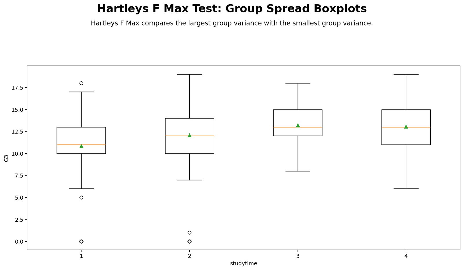
Detailed interpretation

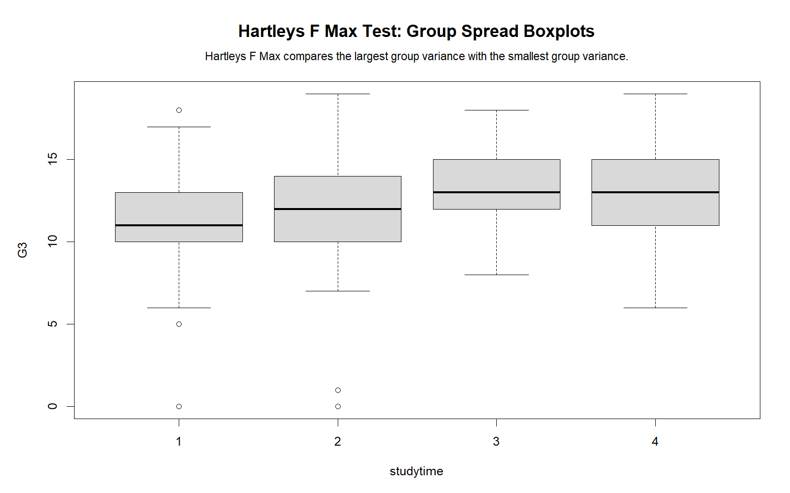
This boxplot shows the distribution of G3 inside each studytime group. The median, interquartile range, whiskers and possible outliers allow the reader to see whether one group appears more variable than another. Studytime group 3 appears tighter than several other groups, which explains why it becomes the smallest-variance group in the F Max calculation.

The chart also reminds us that Hartley’s F Max Test is a spread test, not a mean comparison test. If the research question is about average G3 scores rather than variance, a separate mean-comparison method is needed. The boxplot is still useful because variance assumptions often affect ANOVA-style interpretation.

Decision/reporting conclusion: The boxplots suggest some variance differences, but the visual spread is not extreme enough by itself to conclude a serious homogeneity violation. The formal F Max result and Monte Carlo p-value should guide the final decision.

Python Chart 2: Group Variance Comparison

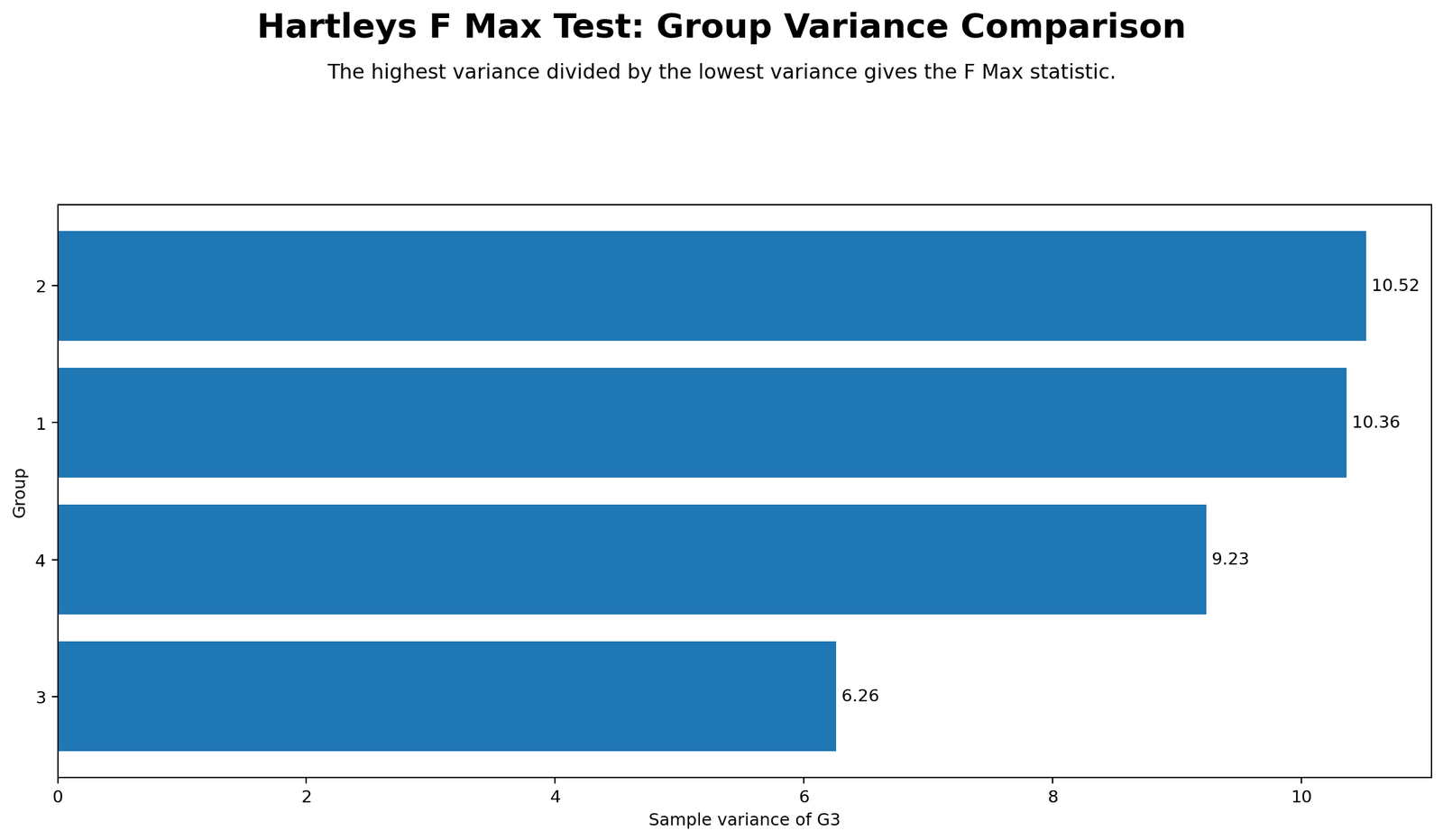
Detailed interpretation

This chart displays the actual sample variances used for the test. Studytime group 2 has the largest variance at approximately 10.5179, while studytime group 3 has the smallest variance at approximately 6.2605. Groups 1 and 4 fall between these values.

Hartley’s F Max Test uses only the largest and smallest variance in its statistic. Therefore, the most important comparison is group 2 versus group 3. The other group variances help explain the overall spread pattern but do not directly define the numerator or denominator of the F Max statistic.

Decision/reporting conclusion: The chart identifies group 2 as the maximum-variance group and group 3 as the minimum-variance group. These values produce the observed Hartley’s F Max statistic of approximately 1.6800.

Python Chart 3: Smallest vs Largest Variance

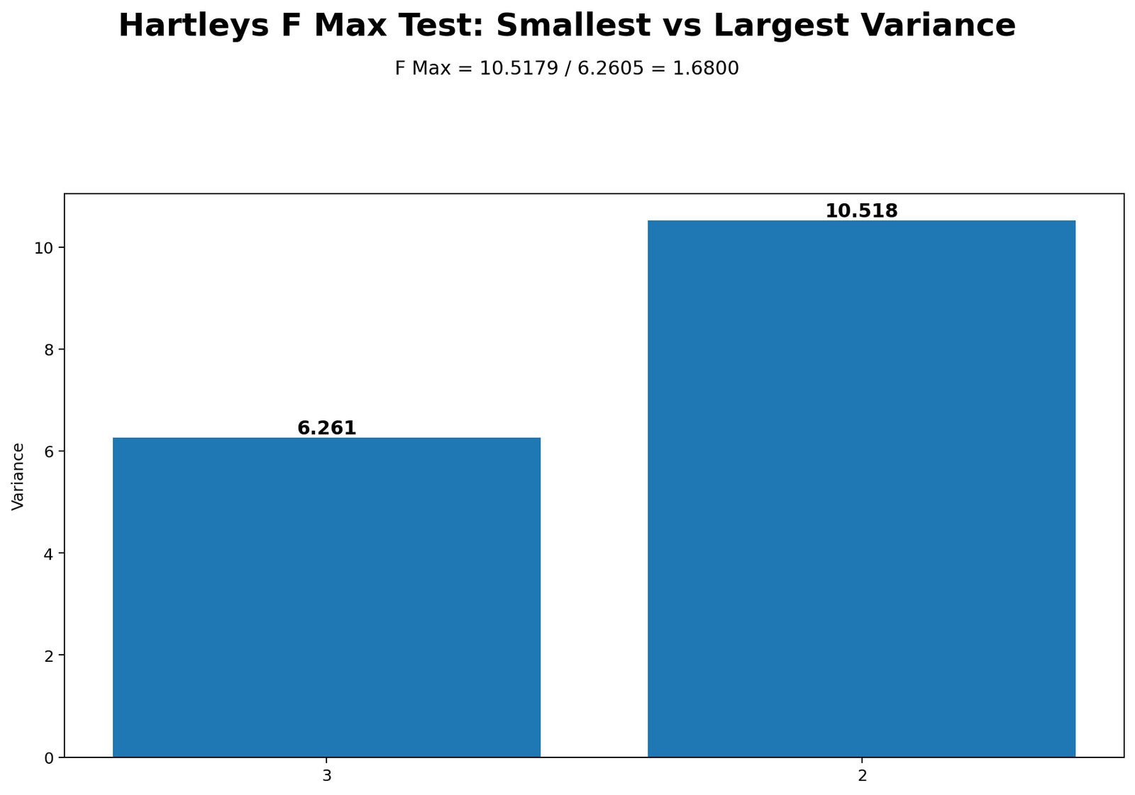
Detailed interpretation

This chart reduces the test to its core calculation. The smallest variance is approximately 6.2605, and the largest variance is approximately 10.5179. Dividing the largest variance by the smallest variance gives F_max ≈ 1.6800.

A ratio of 1.68 indicates that the largest observed group variance is meaningfully larger than the smallest observed group variance. However, the practical size of the ratio is not the full statistical decision. The ratio must be compared with a reference distribution or critical value.

Decision/reporting conclusion: The computed Hartley’s F Max statistic is approximately 1.6800. This value is interpreted as a variance ratio and then evaluated through the Monte Carlo reference distribution.

Python Chart 4: Monte Carlo Reference Distribution

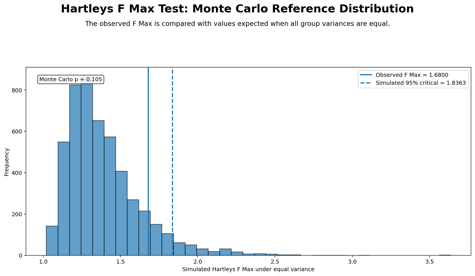
Detailed interpretation

The Monte Carlo reference distribution shows what F Max values can occur when the null hypothesis of equal population variances is true. The observed value is approximately 1.6800. The simulated 95% critical value is higher than the observed statistic, and the approximate p-value is about .105.

This means the observed statistic is not unusually large under the equal-variance assumption. A ratio at least this large can occur with reasonable frequency due to sampling variation.

Decision/reporting conclusion: Because p ≈ .105 is greater than .05, the test fails to reject the null hypothesis. The equal-variance assumption is not flagged as seriously violated by this Hartley F Max analysis.

Python Chart 5: Group Size and Variance

Detailed interpretation

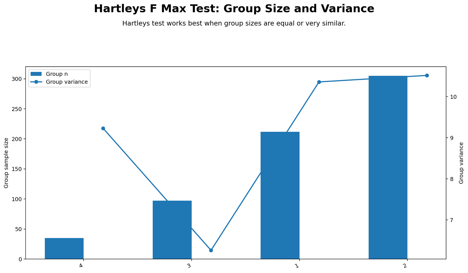
Hartley’s F Max Test performs best when group sizes are equal or similar. This chart compares each studytime group’s sample size with its variance. It helps identify whether a small group may be producing an unstable variance estimate.

The group-size context matters because unequal sample sizes can make simple variance-ratio interpretation less reliable. In this example, the largest variance is not produced only by the smallest group, which makes the result easier to interpret, but the imbalance still deserves caution.

Decision/reporting conclusion: Group sizes are not perfectly balanced, so the Hartley result should be supported with robust checks. The main decision remains non-significant, but Levene and Brown-Forsythe checks are useful additions.

Python Chart 6: Hartley’s F Max Across Groupings

Detailed interpretation

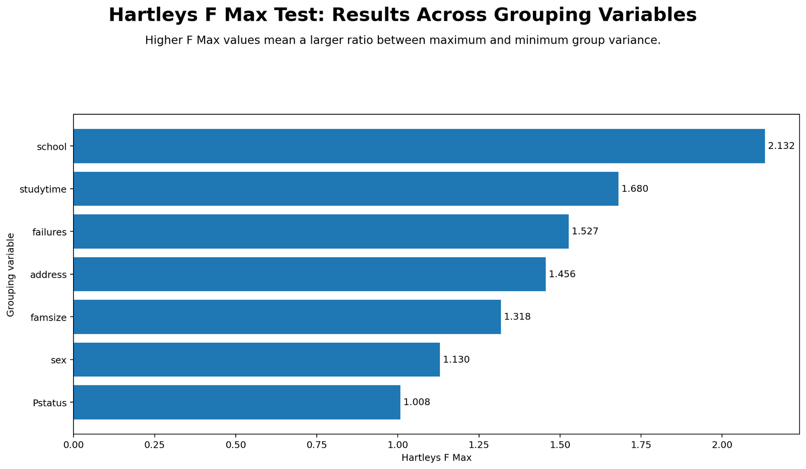
This chart expands the analysis beyond studytime and shows how F Max values change when G3 is grouped by variables such as school, failures, address, famsize, sex and Pstatus. A higher F Max value indicates a larger difference between the largest and smallest group variance for that grouping structure.

This is useful as a screening view. Variance assumptions are tied to the specific grouping or model being analyzed. A variable that looks acceptable for one grouping can show a stronger variance pattern under another grouping.

Decision/reporting conclusion: Studytime shows a moderate F Max value, but the detailed Monte Carlo test does not reject equal variances. Groupings with larger ratios should be checked with robust assumption tests before final modeling.

Python Chart 7: Normality Context Distribution

Detailed interpretation

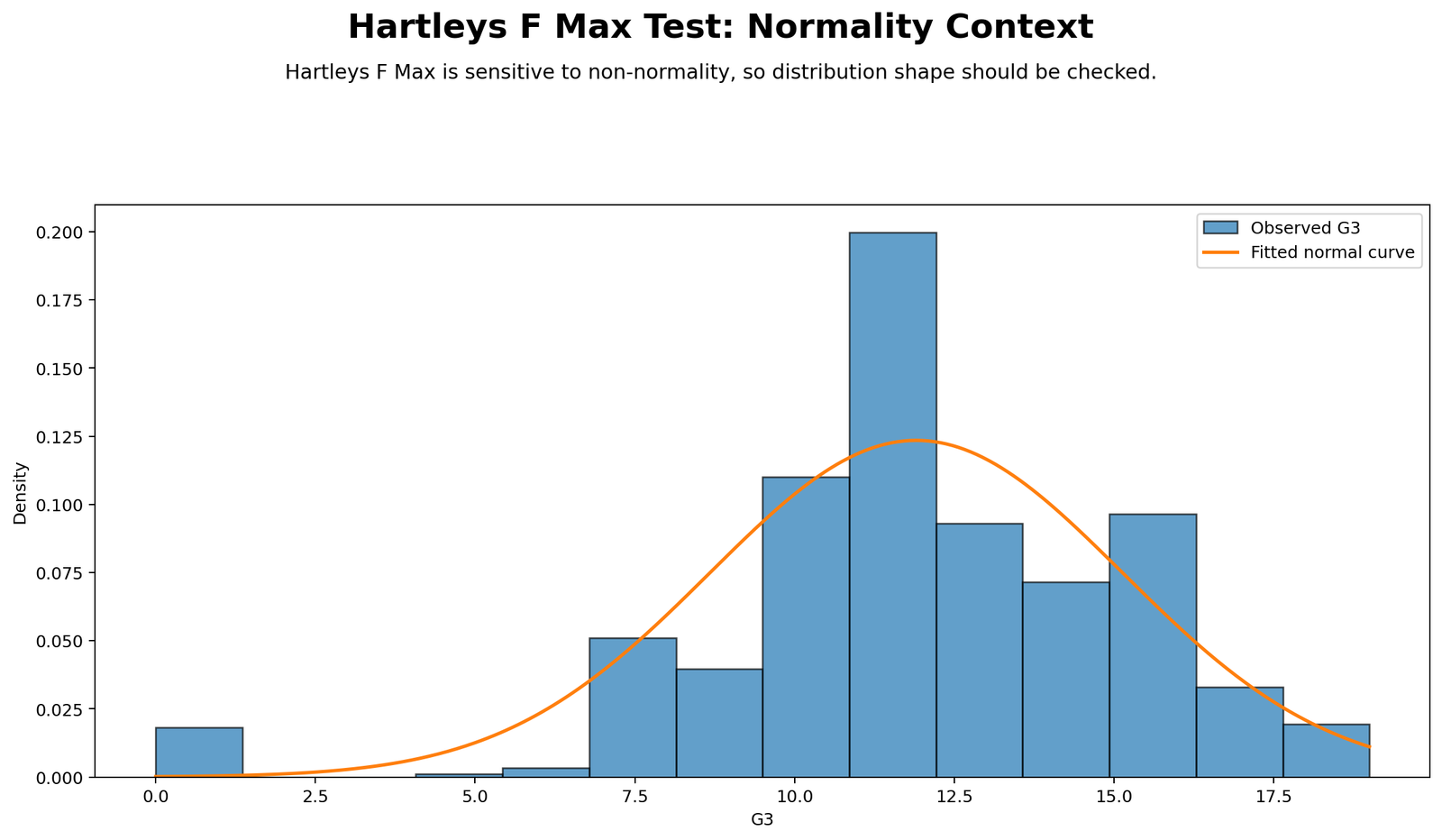
This chart shows the distribution of G3 with a normality context overlay. Hartley’s F Max Test assumes that the data inside groups are reasonably normal. The distribution is broadly centered, but it is not perfectly normal, so the variance test should be interpreted with caution.

The chart should be read together with formal and visual normality checks. Salar Cafe recommends combining the histogram with Q-Q plots, P-P plots, and normality tests when writing a full assumption report.

Decision/reporting conclusion: The normality context is acceptable for teaching and reporting, but not perfect. Since the F Max result is non-significant, the equal variance assumption is not rejected, while robust confirmation remains recommended.

R Chart-by-Chart Validation

The R charts validate the same conclusion using a separate workflow. This is important for reproducibility because the SPSS, Python and R interpretations all point to the same practical result: the observed F Max is approximately 1.68, and the equal-variance assumption is not rejected at the .05 level.

R Chart 1: Group Spread Boxplots

Detailed interpretation

The R boxplot confirms the same spread pattern shown in Python. Studytime group 3 appears more compact, while other studytime groups show wider spread. This supports the variance ranking used in the F Max calculation.

Decision/reporting conclusion: R confirms visible spread differences, but visual evidence alone is not enough. The formal F Max and Monte Carlo p-value still lead to a non-significant conclusion.

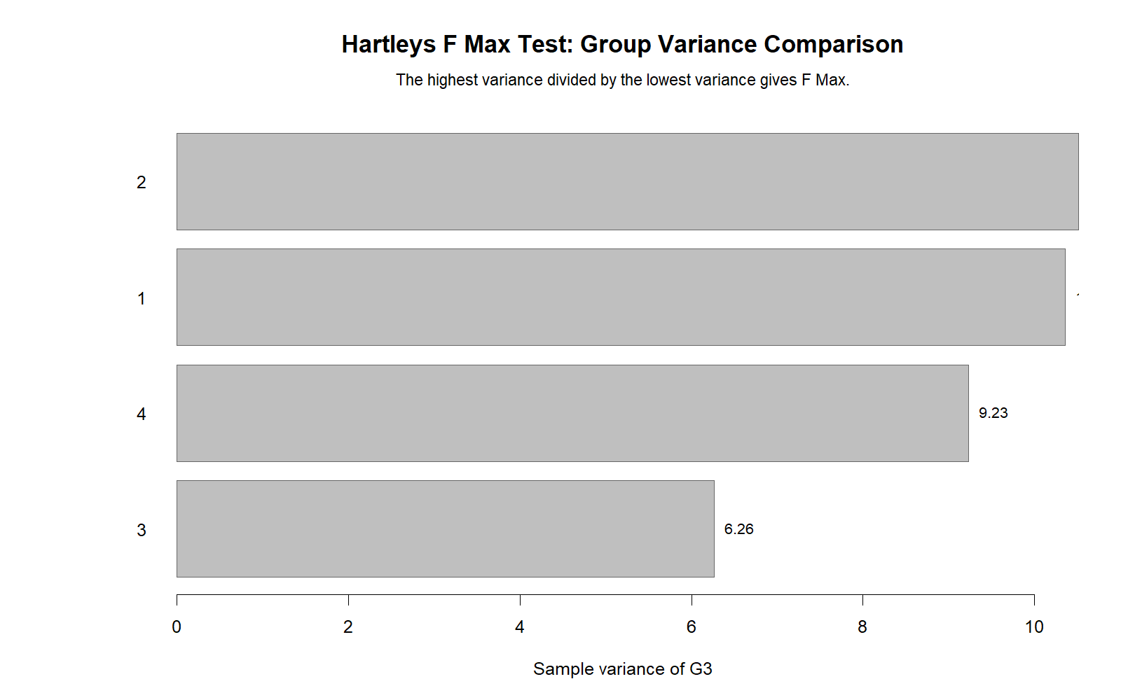
R Chart 2: Group Variance Comparison

Detailed interpretation

This R chart confirms that studytime group 2 has the largest G3 variance and studytime group 3 has the smallest G3 variance. The same max/min pair drives the Hartley statistic in both Python and R.

Decision/reporting conclusion: R validates the Python variance ranking and confirms the core calculation behind F Max ≈ 1.6800.

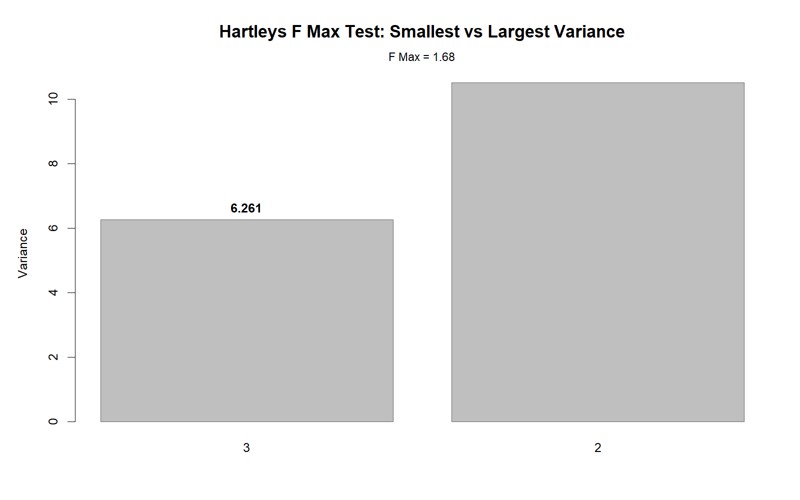
R Chart 3: Smallest vs Largest Variance

Detailed interpretation

The chart isolates the two group variances that define the Hartley’s F Max statistic. It confirms that the maximum variance divided by the minimum variance gives an observed ratio close to 1.68.

Decision/reporting conclusion: R confirms the observed Hartley F Max statistic and supports the same interpretation as the Python and SPSS workflows.

R Chart 4: Monte Carlo Reference Distribution

Detailed interpretation

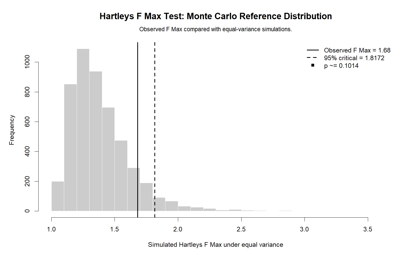
The R Monte Carlo chart compares the observed F Max statistic with simulated F Max values under the equal-variance assumption. The observed statistic is below the simulated 95% critical value, and the approximate p-value is around .10.

Small differences between Python and R simulation values can occur because Monte Carlo estimates depend on random simulation. The substantive conclusion remains unchanged.

Decision/reporting conclusion: R validates the non-significant result. The null hypothesis of equal variances is not rejected.

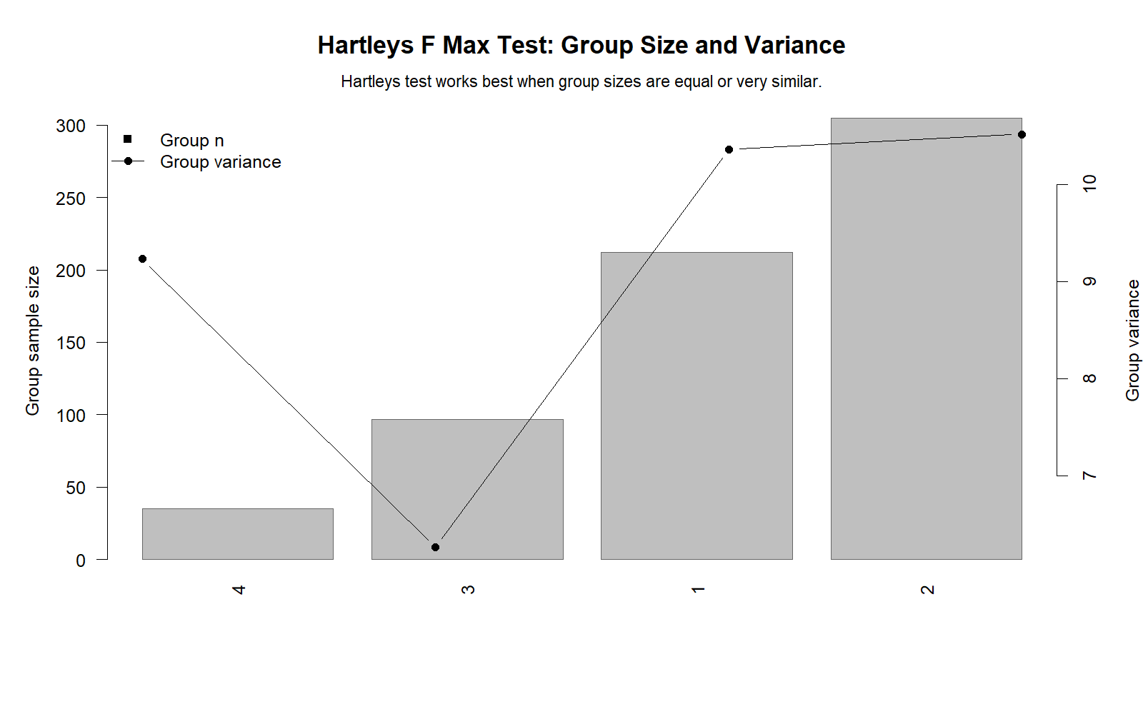
R Chart 5: Group Size and Variance

Detailed interpretation

This chart validates that studytime groups are not perfectly equal in size. Unequal sample sizes make it important to interpret Hartley’s F Max Test carefully and preferably alongside robust variance tests.

Decision/reporting conclusion: R confirms group-size imbalance. The F Max result is still non-significant, but robust checks are recommended for careful research reporting.

R Chart 6: Hartley’s F Max Across Groupings

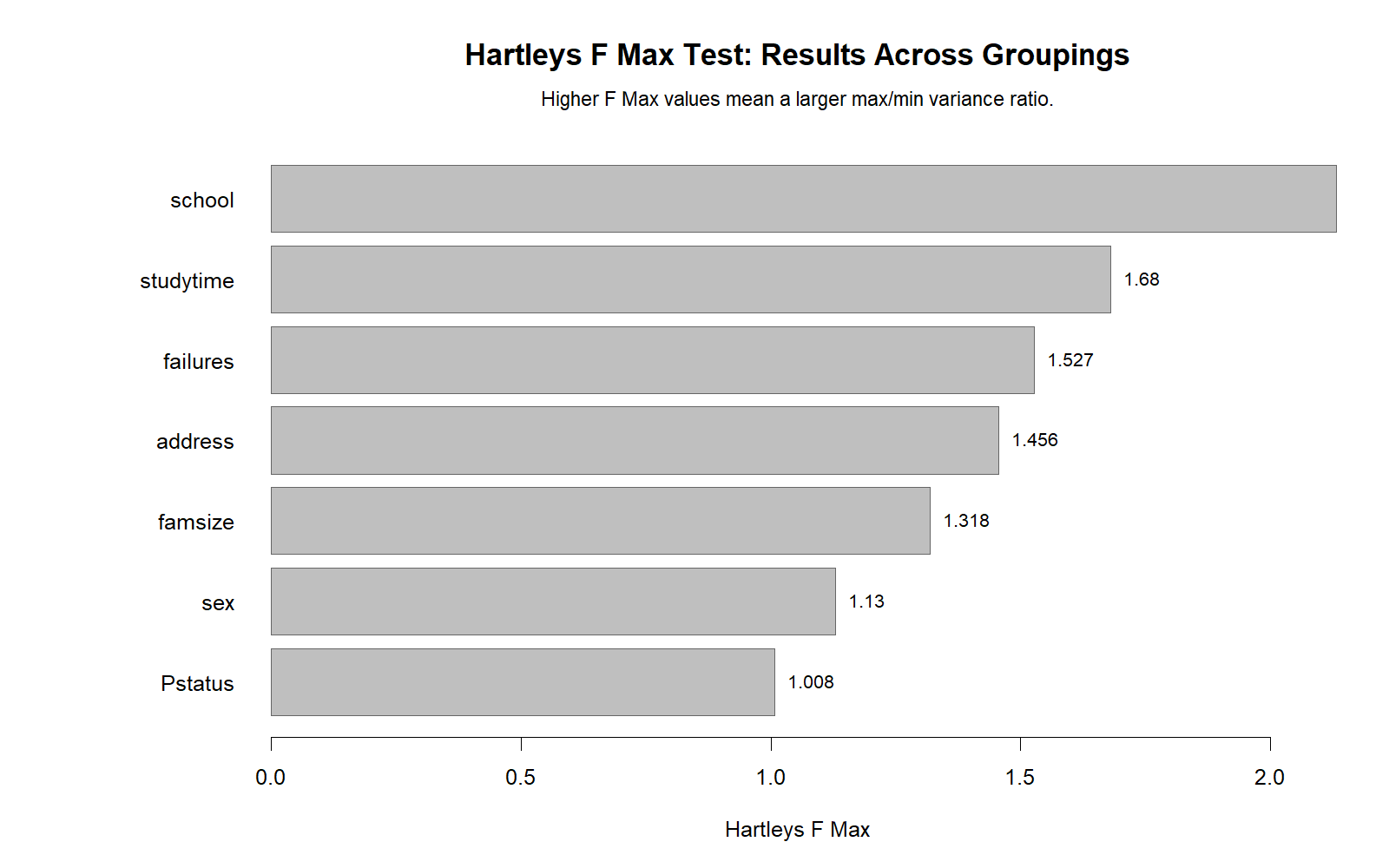
Detailed interpretation

The R screening chart confirms that F Max changes across grouping variables. This is important because variance assumptions are model-specific. The grouping variable used in the main analysis should be the one checked for homogeneity.

Decision/reporting conclusion: R confirms that studytime has a moderate variance ratio, while other grouping variables may require separate assumption checks depending on the final model.

R Chart 7: Normality Context Distribution

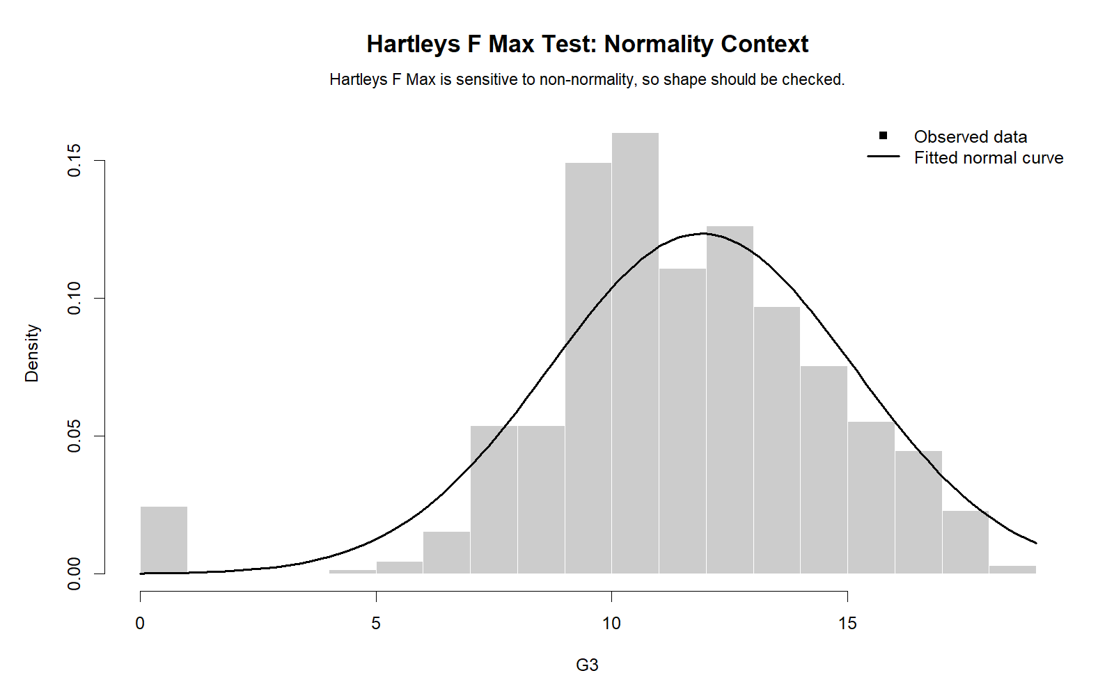
Detailed interpretation

The R normality context chart confirms that G3 is not perfectly normal. Because Hartley’s F Max Test is sensitive to non-normality, this chart provides essential context for the final interpretation.

Decision/reporting conclusion: R supports a cautious interpretation. The variance test is not significant, but the report should acknowledge normality context and recommend robust checks where necessary.

SPSS, Python, R and Excel Workflows

SPSS Workflow

1. Open the cleaned dataset in SPSS.
2. Confirm that G3 is numeric and studytime is categorical.
3. Use descriptive procedures or aggregation to calculate variance of G3 within each studytime group.
4. Identify the largest group variance and smallest group variance.
5. Calculate F Max = largest variance / smallest variance.
6. Interpret the statistic using a reference table, critical value or Monte Carlo simulation.
7. Export the SPSS output PDF for reporting and documentation.

Python Workflow

1. Load the dataset using pandas.
2. Drop missing values for G3 and studytime.
3. Calculate group count, mean, variance and standard deviation.
4. Compute the F Max statistic.
5. Simulate equal-variance data to build a Monte Carlo reference distribution.
6. Create boxplots, variance charts, F Max calculation charts and normality context plots.
7. Write the final decision using the observed statistic and p-value.

R Workflow

1. Read the dataset with read.csv().
2. Convert studytime to a factor.
3. Calculate group variances with tapply() or dplyr.
4. Compute max(variance) / min(variance).
5. Simulate a Monte Carlo reference distribution.
6. Validate the Python and SPSS-style results with R charts.

Excel Workflow

1. Place G3 values and studytime group labels in Excel.
2. Separate or filter G3 values by studytime group.
3. Use VAR.S() to calculate sample variance for each group.
4. Use MAX() and MIN() to find the largest and smallest variance.
5. Divide the largest variance by the smallest variance.
6. Report the F Max statistic and interpret it with a critical value or simulation p-value.

SPSS Syntax, Python Code, R Code and Excel Formulas

SPSS Syntax for Hartley’s F Max Test

* Hartley's F Max Test workflow in SPSS.
* Dataset should include G3 and studytime.

SET PRINTBACK=OFF MPRINT=OFF.

DATASET ACTIVATE DataSet1.

TITLE "Hartley's F Max Test: G3 Variance by Studytime".

FREQUENCIES VARIABLES=studytime.

DESCRIPTIVES VARIABLES=G3
  /STATISTICS=MEAN STDDEV VARIANCE MIN MAX.

AGGREGATE
  /OUTFILE=* MODE=ADDVARIABLES
  /BREAK=studytime
  /group_n = N(G3)
  /group_mean = MEAN(G3)
  /group_sd = SD(G3)
  /group_variance = VARIANCE(G3).

SORT CASES BY studytime.

REPORT FORMAT=LIST AUTOMATIC ALIGN(CENTER)
  /VARIABLES=studytime group_n group_mean group_sd group_variance
  /TITLE "Hartley's F Max Test: Group Variance Summary for G3 by Studytime".

* Manual F Max calculation:
* F Max = largest group_variance / smallest group_variance.
* Example:
* F Max = 10.5179 / 6.2605 = 1.6800.

OUTPUT EXPORT
  /CONTENTS EXPORT=VISIBLE LAYERS=PRINTSETTING MODELVIEWS=PRINTSETTING
  /PDF DOCUMENTFILE="Hartleys-F-Max-Test-SPSS-Output.pdf"
  /EMBEDBOOKMARKS YES
  /EMBEDFONTS YES.

Python Code for Hartley’s F Max Test

import numpy as np
import pandas as pd

df = pd.read_csv("spss_ready_data.csv")

outcome = "G3"
group = "studytime"

data = df[[outcome, group]].dropna().copy()

summary = (
    data.groupby(group)[outcome]
    .agg(n="count", mean="mean", variance="var", sd="std")
    .reset_index()
)

largest_variance = summary["variance"].max()
smallest_variance = summary["variance"].min()
largest_group = summary.loc[summary["variance"].idxmax(), group]
smallest_group = summary.loc[summary["variance"].idxmin(), group]

fmax = largest_variance / smallest_variance

print(summary)
print("Largest variance group:", largest_group, largest_variance)
print("Smallest variance group:", smallest_group, smallest_variance)
print("Hartley's F Max:", fmax)

# Monte Carlo reference distribution
rng = np.random.default_rng(12345)
group_sizes = summary["n"].to_numpy()
n_sims = 5000
sim_fmax = []

for _ in range(n_sims):
    variances = []
    for n in group_sizes:
        simulated = rng.normal(loc=0, scale=1, size=int(n))
        variances.append(np.var(simulated, ddof=1))
    sim_fmax.append(max(variances) / min(variances))

sim_fmax = np.array(sim_fmax)
p_value = np.mean(sim_fmax >= fmax)
critical_95 = np.quantile(sim_fmax, 0.95)

print("Monte Carlo p-value:", p_value)
print("Simulated 95% critical value:", critical_95)

if p_value < 0.05:
    print("Reject H0: evidence of unequal variances.")
else:
    print("Fail to reject H0: no strong evidence of unequal variances.")

R Code for Hartley's F Max Test

# Hartley's F Max Test in R

df <- read.csv("spss_ready_data.csv")

outcome <- "G3"
group <- "studytime"

data <- df[, c(outcome, group)]
data <- na.omit(data)
data[[group]] <- as.factor(data[[group]])

group_n <- tapply(data[[outcome]], data[[group]], length)
group_mean <- tapply(data[[outcome]], data[[group]], mean)
group_var <- tapply(data[[outcome]], data[[group]], var)
group_sd <- tapply(data[[outcome]], data[[group]], sd)

summary_table <- data.frame(
  group = names(group_var),
  n = as.numeric(group_n),
  mean = as.numeric(group_mean),
  variance = as.numeric(group_var),
  sd = as.numeric(group_sd)
)

print(summary_table)

largest_variance <- max(summary_table$variance)
smallest_variance <- min(summary_table$variance)
fmax <- largest_variance / smallest_variance

cat("Largest variance:", largest_variance, "\n")
cat("Smallest variance:", smallest_variance, "\n")
cat("Hartley's F Max:", fmax, "\n")

set.seed(12345)
n_sims <- 5000
group_sizes <- summary_table$n
sim_fmax <- numeric(n_sims)

for (i in seq_len(n_sims)) {
  variances <- sapply(group_sizes, function(n) var(rnorm(n, mean = 0, sd = 1)))
  sim_fmax[i] <- max(variances) / min(variances)
}

p_value <- mean(sim_fmax >= fmax)
critical_95 <- quantile(sim_fmax, 0.95)

cat("Monte Carlo p-value:", p_value, "\n")
cat("Simulated 95% critical value:", critical_95, "\n")

if (p_value < 0.05) {
  cat("Reject H0: evidence of unequal variances.\n")
} else {
  cat("Fail to reject H0: no strong evidence of unequal variances.\n")
}

Excel Formulas for Hartley's F Max Test

Assume G3 values for four studytime groups are arranged in B:E.

Variance for group 1:
=VAR.S(B2:B213)

Variance for group 2:
=VAR.S(C2:C306)

Variance for group 3:
=VAR.S(D2:D98)

Variance for group 4:
=VAR.S(E2:E36)

Largest variance:
=MAX(B10:E10)

Smallest variance:
=MIN(B10:E10)

Hartley's F Max:
=MAX(B10:E10)/MIN(B10:E10)

Interpretation:
If F Max is close to 1, group variances are similar.
If F Max is large, check a critical value, simulation p-value, Levene test or Brown-Forsythe test.

APA Reporting Wording for Hartley's F Max Test

When reporting Hartley's F Max Test, include the outcome variable, grouping variable, largest variance, smallest variance, observed F Max statistic, reference method, p-value and decision. Avoid saying “the null hypothesis is accepted.” The correct phrase is “failed to reject the null hypothesis.”

APA-Style Report

Short Report Sentence

Decision Language

Common Mistakes in Hartley's F Max Test Interpretation

When to Use Hartley's F Max Test

Use Hartley's F Max Test when you have a continuous outcome variable, several independent groups and a need to check whether the group variances are approximately equal. It is especially useful in teaching, introductory statistics, and transparent assumption checking because the formula is simple and easy to explain.

For advanced applied work, connect Hartley's F Max Test with broader reporting tools such as effect size, central limit theorem, and clinical trial data analysis using R when the research context involves treatment groups, outcome variability or assumption-sensitive modeling.

Downloads and Resources for Hartley's F Max Test

Use the SPSS output PDF, Python charts and R validation charts below to support your WordPress post, classroom explanation, student assignment, research report or data-analysis service page.

Related Internal Links for Salar Cafe Statistical Guides

Use these related Salar Cafe guides to connect Hartley's F Max Test with normality tests, variance tests, transformation methods, regression diagnostics, descriptive statistics, hypothesis testing, confidence intervals and reporting.