
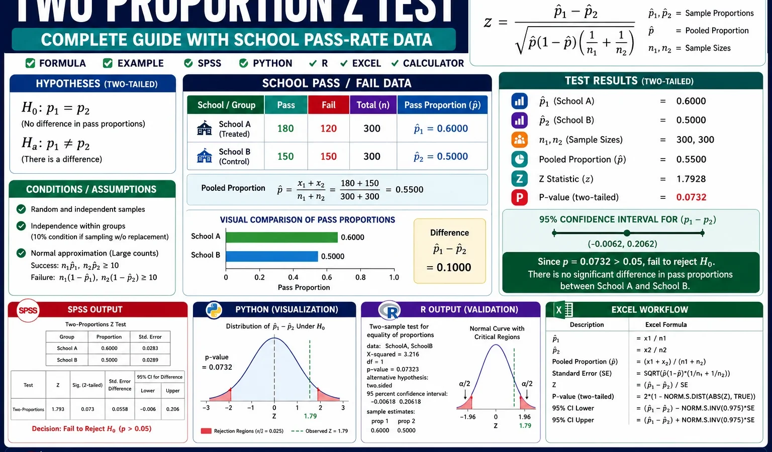
Hypothesis Test for Comparing Two Proportions
Two Proportion Z Test is used to test whether two independent population proportions are significantly different. This guide explains the two sample z test for proportions with formula, assumptions, conditions, p-value, confidence interval, SPSS image output, Python charts, R validation charts and Excel workflow using school pass-rate data where pass = G3 ≥ 10.
Quick Answer: Two Proportion Z Test Result
The Two Proportion Z Test was performed to compare the final exam pass proportion between two schools: GP and MS. A student was coded as pass if G3 ≥ 10 and fail if G3 < 10.
In the GP school, 391 students passed out of 423, giving p1 = 0.9243. In the MS school, 158 students passed out of 226, giving p2 = 0.6991. The observed difference was p1 − p2 = 0.2252, meaning the GP pass proportion was about 22.5 percentage points higher than the MS pass proportion.
The pooled proportion used for the hypothesis test was 0.8459. The pooled standard error was 0.0297. The z statistic was z = 7.5717, and the two-tailed p-value was approximately 3.68 × 10⁻¹⁴. In a final report, this should be written as p < .001. The 95% confidence interval for the difference in pass proportions was [0.1603, 0.2901].
Final conclusion: Since p < .001, reject the null hypothesis. The sample provides strong evidence that the pass proportions are significantly different between GP and MS. Because the observed difference is positive, the GP school has a significantly higher pass proportion than the MS school.
Important reporting note: Some software may display very small p-values as .000. Do not write p = .000. The correct reporting style is p < .001.
Table of Contents
- What Is a Two Proportion Z Test?
- When to Use Two Proportion Z Test
- Null and Alternative Hypothesis
- Two Proportion Z Test Formula
- Conditions and Assumptions
- Dataset and Variable Coding
- Verified Results Summary
- SPSS Image Output and Interpretation
- Python Charts and Interpretation
- R Validation Charts and Interpretation
- Overall Image Interpretation
- How to Run the Test in SPSS, Python, R and Excel
- How to Report the Two Proportion Z Test
- Common Mistakes
- FAQs
What Is a Two Proportion Z Test?
A Two Proportion Z Test is a statistical hypothesis test used to compare two independent sample proportions. It is also called a two sample z test for proportions, two sample z proportion test or z test for two proportions.
The test is used when the outcome variable has two categories, such as pass/fail, yes/no, success/failure or converted/not converted. The grouping variable must have two independent groups. In this example, the outcome is final exam status and the grouping variable is school. The two school groups are GP and MS.
The main question is: Is the pass proportion at GP significantly different from the pass proportion at MS? The test compares p1 and p2. If the difference between the two sample proportions is large relative to its standard error, the z statistic becomes large and the p-value becomes small.
For background concepts, see Null and Alternative Hypothesis, P Value, Z Score, Standard Error, Standard Normal Distribution and Cross Tabulation.
When Should You Use a Two Proportion Z Test?
Use a two proportion z test when you want to compare two independent proportions. It is appropriate when the outcome is binary and each case belongs to only one of the two groups.
| Situation | Use Two Proportion Z Test? | Reason |
|---|---|---|
| Comparing pass rate between GP and MS schools | Yes | The outcome is pass/fail and there are two independent school groups. |
| Comparing conversion rate between two landing pages | Yes | The outcome is converted/not converted and the groups are independent. |
| Comparing support rate between two survey groups | Yes | The outcome is support/no support across two groups. |
| Testing whether one pass proportion differs from 50% | No | That is a one-sample proportion question. Use a One Proportion Z Test. |
| Comparing average G3 score between two schools | No | That is a mean comparison, not a proportion comparison. |
The one proportion vs two proportion z test difference is simple: one proportion z test compares one observed proportion with one benchmark value, while two proportion z test compares two observed proportions from two groups.
Null and Alternative Hypothesis for Two Proportion Z Test
The hypotheses compare the two population proportions. In this example, p1 is the GP pass proportion and p2 is the MS pass proportion.
| Hypothesis | Symbolic form | Meaning in this example |
|---|---|---|
| Null hypothesis | H0: p1 = p2 | The GP and MS population pass proportions are equal. |
| Alternative hypothesis | H1: p1 ≠ p2 | The GP and MS population pass proportions are different. |
| Equivalent difference form | H0: p1 − p2 = 0 | There is no population pass-rate difference between schools. |
| Decision rule | Reject H0 if p-value < α | Using α = .05, reject H0 because p < .001. |
This example uses a two-tailed two proportion z test because the alternative hypothesis says the proportions are different. A right-tailed test would use H1: p1 > p2, and a left-tailed test would use H1: p1 < p2.
Two Proportion Z Test Formula and Exact Calculation
The two proportion z test formula compares two sample proportions using a pooled standard error under the null hypothesis.
z = (p1 - p2) / SEpooled

p1 = x1 / n1
p2 = x2 / n2

pooled p = (x1 + x2) / (n1 + n2)

SEpooled = sqrt[pooled p × (1 - pooled p) × (1/n1 + 1/n2)]
For this worked example:
| Component | Exact value | Explanation |
|---|---|---|
| Group 1 | GP | First school group. |
| Group 2 | MS | Second school group. |
| GP successes | x1 = 391 | GP students who passed. |
| GP sample size | n1 = 423 | Total GP students. |
| MS successes | x2 = 158 | MS students who passed. |
| MS sample size | n2 = 226 | Total MS students. |
| GP pass proportion | p1 = 391/423 = 0.9243 | About 92.4% of GP students passed. |
| MS pass proportion | p2 = 158/226 = 0.6991 | About 69.9% of MS students passed. |
| Difference | p1 − p2 = 0.2252 | GP is 22.5 percentage points higher than MS. |
| Pooled proportion | 0.8459 | Combined pass proportion under H0. |
| Pooled standard error | 0.0297 | Standard error used for the z statistic. |
| Z statistic | 7.5717 | Observed difference is 7.57 pooled standard errors above zero. |
| Two-tailed p-value | p < .001 | Reject the null hypothesis. |
p1 = 391 / 423 = 0.9243
p2 = 158 / 226 = 0.6991

difference = p1 - p2
difference = 0.9243 - 0.6991
difference = 0.2252

pooled p = (391 + 158) / (423 + 226)
pooled p = 549 / 649
pooled p = 0.8459

SEpooled = sqrt[0.8459 × (1 - 0.8459) × (1/423 + 1/226)]
SEpooled = 0.0297

z = 0.2252 / 0.0297
z = 7.5717
Why Do We Pool for the Two-Proportion Z-Test?
The test pools the two sample proportions because the null hypothesis says the two population proportions are equal. If H0: p1 = p2 is true, both groups estimate one common population proportion. That common estimate is the pooled proportion.
The confidence interval for the difference is usually calculated with the unpooled standard error because the interval estimates the actual size of the difference, not the null condition of equality. In this example, the 95% confidence interval for p1 − p2 is [0.1603, 0.2901].
Conditions and Assumptions for Two Proportion Z Test
The conditions for two proportion z test explain when the z approximation is appropriate. These conditions should be checked before interpreting the p-value.
| Condition | How to check it | This example |
|---|---|---|
| Binary outcome | The outcome must have two categories. | Pass = G3 ≥ 10; Fail = G3 < 10. |
| Two independent groups | Each case belongs to only one group. | Each student belongs to either GP or MS. |
| Independent observations | Each row should represent a separate case. | Each row is treated as one student record. |
| Large-sample condition | Each group should have enough expected successes and failures. | All school pass/fail counts are large enough for the z approximation. |
| No repeated measurement of the same case | The two groups should not be paired or matched. | GP and MS are independent school groups. |
If the sample counts are very small, an exact method may be safer. With 423 GP students and 226 MS students, the sample size condition is satisfied.
Dataset and Variable Coding
This worked example uses student performance data. The final grade variable is G3. A binary pass/fail outcome was created from G3. A student was coded as pass if G3 ≥ 10 and fail if G3 < 10.
| Item | Value | Explanation |
|---|---|---|
| Outcome variable | pass_final | Binary pass/fail variable created from G3. |
| Success definition | G3 ≥ 10 | Student passed the final exam. |
| Failure definition | G3 < 10 | Student did not pass the final exam. |
| Grouping variable | school | Two independent school groups: GP and MS. |
| GP group | 391 pass, 32 fail, n = 423 | GP pass proportion = 0.9243. |
| MS group | 158 pass, 68 fail, n = 226 | MS pass proportion = 0.6991. |
External dataset source: UCI Machine Learning Repository: Student Performance dataset.
Verified SPSS, Python and R Results Summary
The SPSS image output, Python charts and R validation charts all support the same decision. GP has a higher pass proportion than MS. The difference is 0.2252, the confidence interval is entirely above zero, and the z statistic is far beyond the usual ±1.96 critical values.
| Statistic | Exact value | Interpretation |
|---|---|---|
| GP pass count | 391 | Students who passed in GP. |
| GP total | 423 | Total GP students. |
| GP pass proportion | 0.9243 | 92.4% passed. |
| MS pass count | 158 | Students who passed in MS. |
| MS total | 226 | Total MS students. |
| MS pass proportion | 0.6991 | 69.9% passed. |
| Difference | 0.2252 | GP is 22.5 percentage points higher. |
| 95% CI for difference | [0.1603, 0.2901] | The interval is entirely above zero. |
| Z statistic | 7.5717 | The result is far into the rejection region. |
| p-value | p < .001 | Reject H0. |
SPSS Image Output and Interpretation
The SPSS image output explains the Two Proportion Z Test visually. These images show the raw school pass/fail counts, the two pass proportions, the confidence interval for the difference, the z statistic on the standard normal curve and subgroup context by sex and study time.
1. SPSS Image: Pass and Fail Counts by School
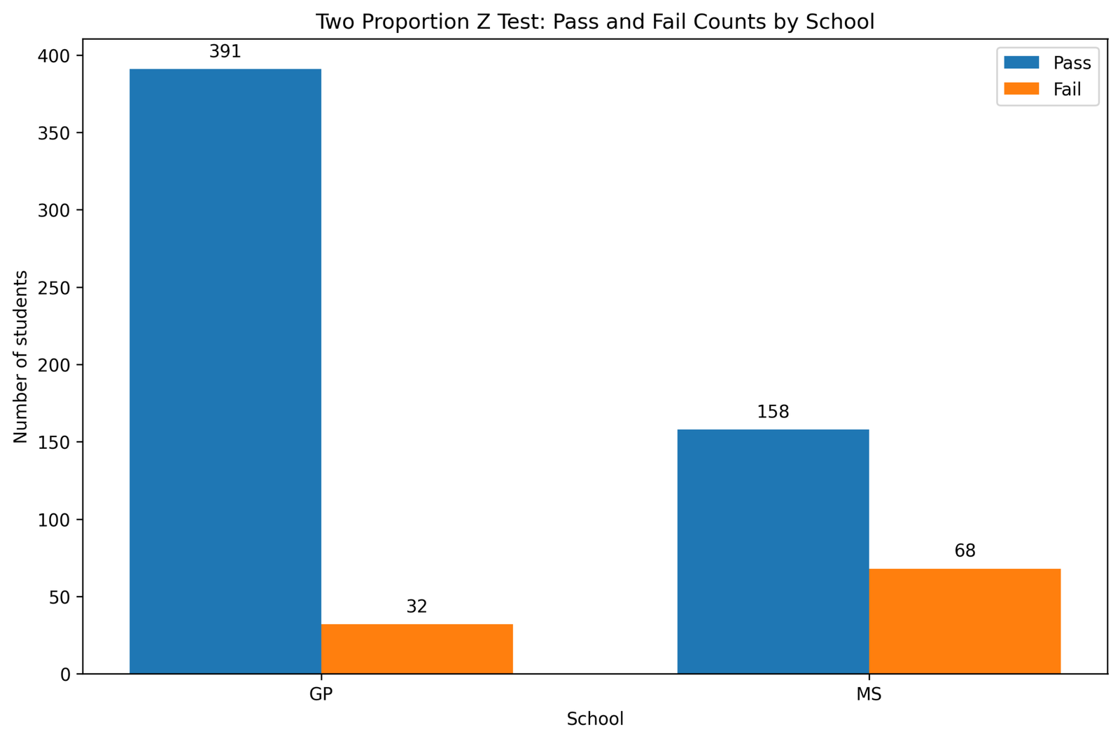
This SPSS image shows the raw counts used in the Two Proportion Z Test. In the GP school, 391 students passed and 32 failed. In the MS school, 158 students passed and 68 failed.
The chart is important because it shows the data before any statistical formula is applied. The GP school has a much larger pass count and a much smaller fail count relative to its total. The MS school still has more passes than failures, but the failure count is much larger relative to its group size.
These counts directly produce the sample proportions: 391/423 = 0.9243 for GP and 158/226 = 0.6991 for MS. Therefore, this image is the foundation of the entire z-test calculation.
2. SPSS Image: Pass Proportion Comparison by School
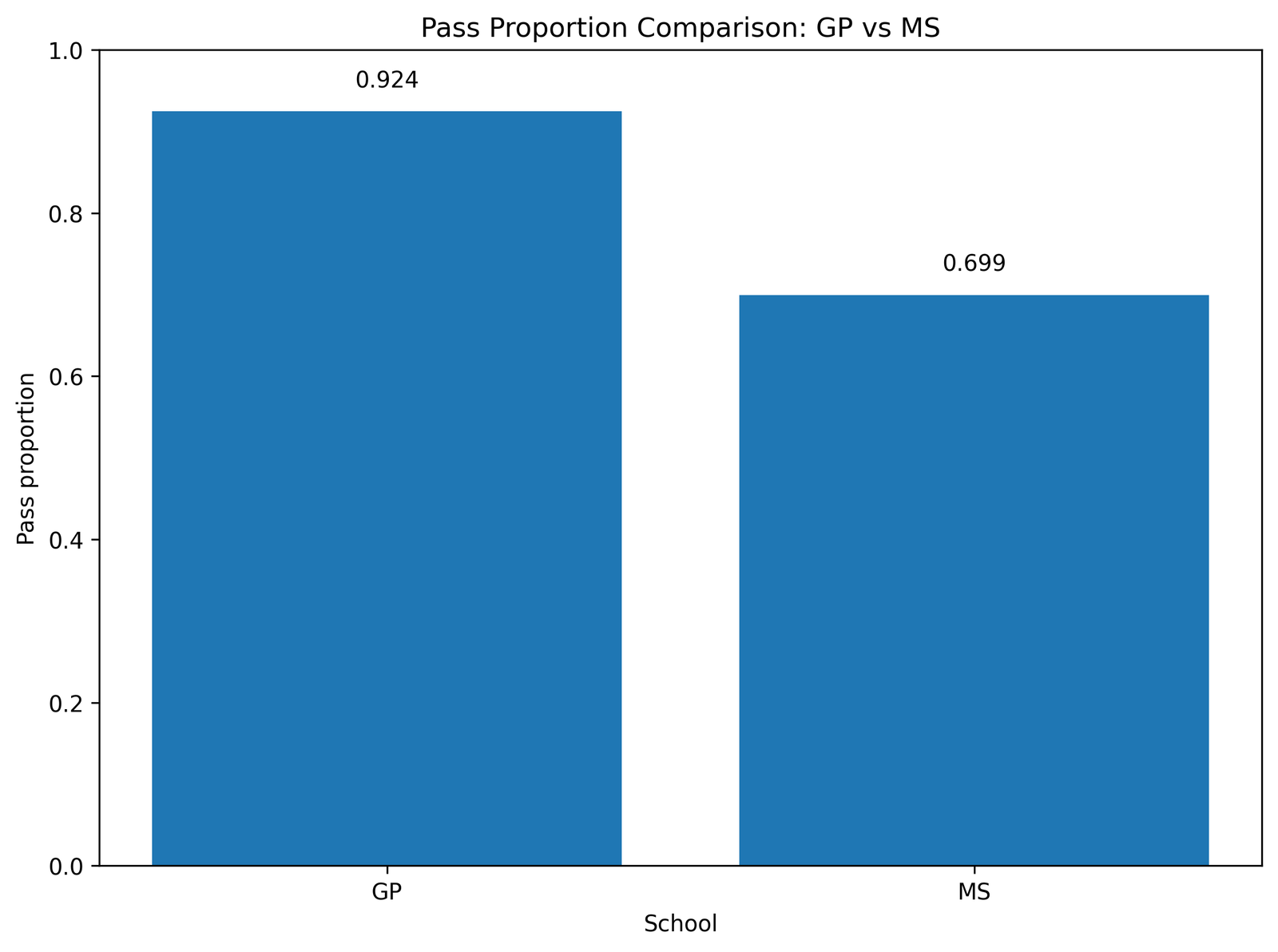
This SPSS image compares the two observed pass proportions. The GP pass proportion is 0.924, while the MS pass proportion is 0.699. The difference is 0.225, meaning GP is about 22.5 percentage points higher than MS.
This image shows the central comparison in the Two Proportion Z Test. The null hypothesis says the two population pass proportions are equal. The observed data show a clear difference between the two schools.
The chart also gives practical meaning to the result. Even before looking at the p-value, the difference is large enough to matter educationally: roughly 92% of GP students passed, compared with roughly 70% of MS students.
3. SPSS Image: Confidence Interval for Difference in Proportions
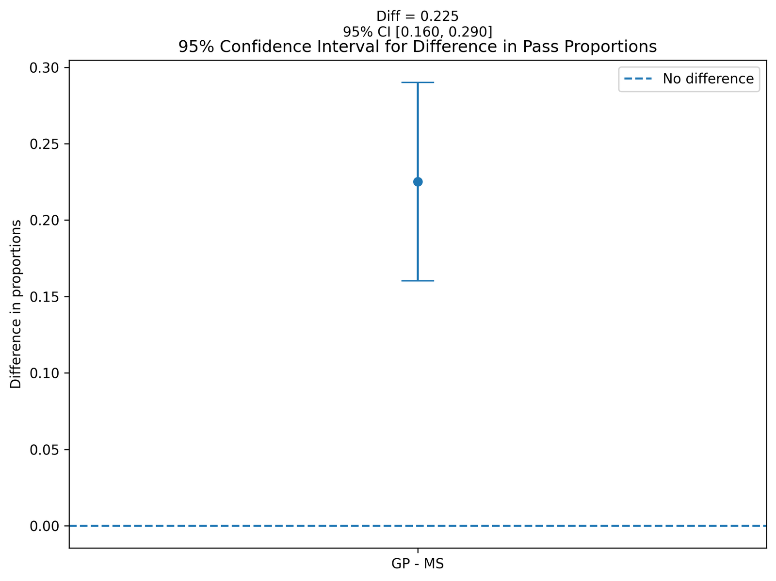
This SPSS image shows the confidence interval for the difference between the two pass proportions. The observed difference is 0.225, and the 95% confidence interval is [0.160, 0.290].
The dashed no-difference line is located at 0. The entire confidence interval is above zero. This means the estimated GP pass proportion is higher than the MS pass proportion even after accounting for sampling uncertainty.
The confidence interval also gives practical size. It suggests that the GP pass proportion is likely between about 16.0 and 29.0 percentage points higher than the MS pass proportion.
4. SPSS Image: Z Statistic on the Standard Normal Curve
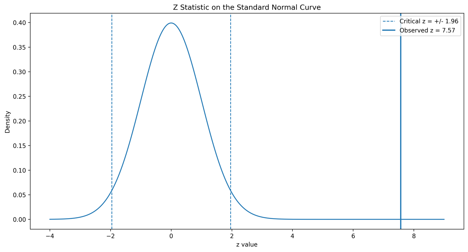
This SPSS image places the test statistic on the standard normal curve. The observed value is z = 7.57. For a two-tailed test at α = .05, the usual critical values are ±1.96.
The observed z statistic is far to the right of +1.96. This means the observed difference in pass proportions is far larger than what would normally be expected if the two population proportions were equal.
The curve image explains why the p-value is extremely small. A z value of 7.57 is deep in the rejection region. Therefore, the test rejects the null hypothesis of equal pass proportions.
5. SPSS Image: Pass/Fail Percentage Composition by School

This SPSS stacked percentage image shows the composition of each school group. GP has a pass percentage of 92.4% and a fail percentage of 7.6%. MS has a pass percentage of 69.9% and a fail percentage of 30.1%.
This chart is useful because it puts both groups on the same 0 to 100% scale. It makes the school difference easier to compare visually than raw counts alone.
The stacked bars show that failure occupies a much larger share of the MS bar than the GP bar. This supports the main conclusion that school is associated with a meaningful difference in pass proportion.
6. SPSS Image: Pass Proportion by Sex Within School
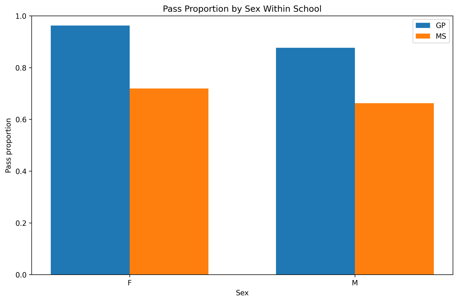
This SPSS image provides subgroup context by sex within school. Among female students, GP has 228 passes out of 237, or 96.2%, while MS has 105 passes out of 146, or 71.9%. Among male students, GP has 163 passes out of 186, or 87.6%, while MS has 53 passes out of 80, or 66.3%.
The chart shows that the GP pass proportion is higher than the MS pass proportion for both female and male students. This supports the overall school comparison because the school difference is not limited to only one sex category.
This image is descriptive context. The formal Two Proportion Z Test compares overall GP and MS pass proportions. If the research question were about sex-by-school interaction, a more detailed model would be needed.
7. SPSS Image: Pass Proportion by Study Time Within School
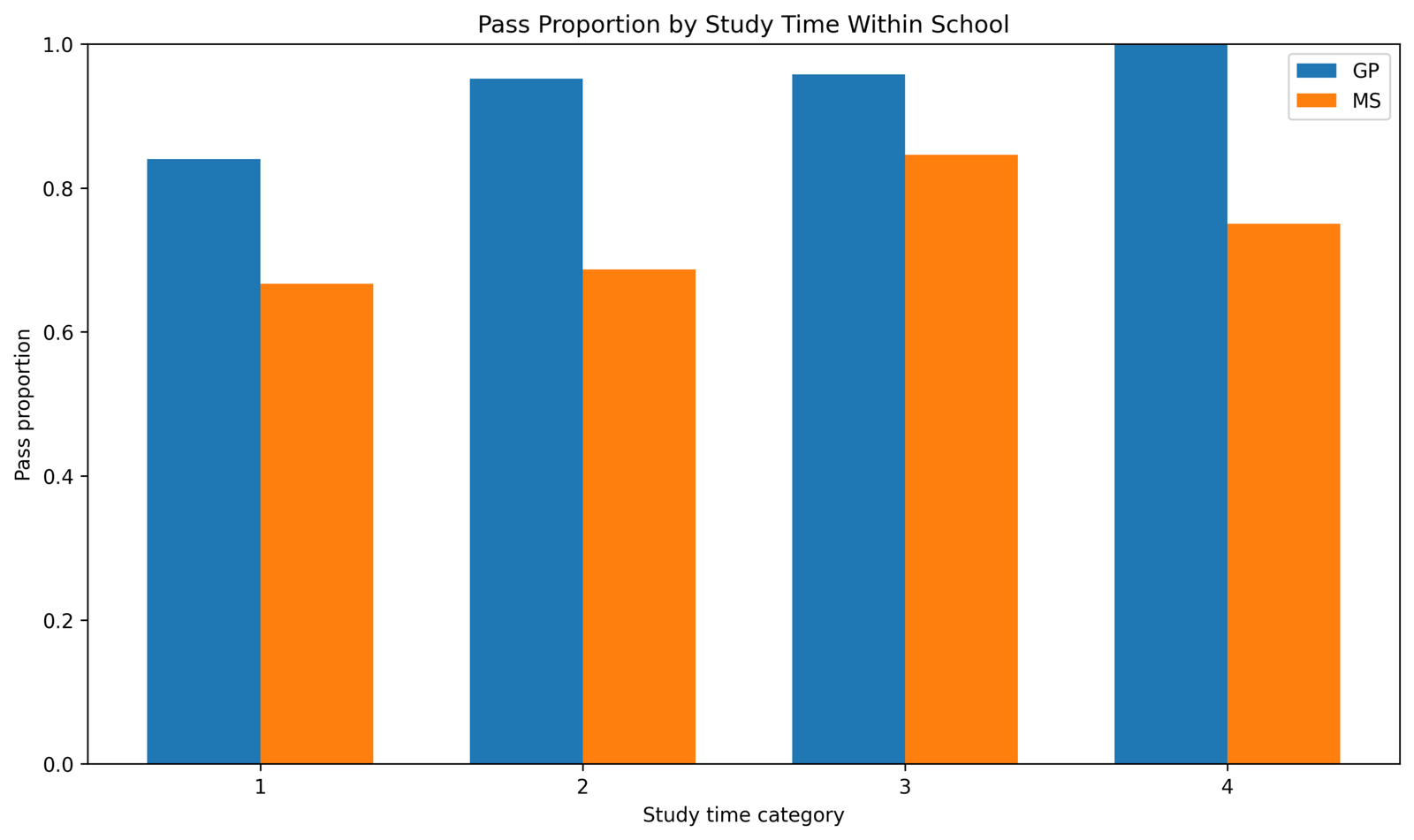
This SPSS image shows pass proportions by study-time category within each school. In study-time category 1, GP has 100/119 = 84.0% passing, while MS has 62/93 = 66.7%. In category 2, GP has 196/206 = 95.1%, while MS has 68/99 = 68.7%. In category 3, GP has 68/71 = 95.8%, while MS has 22/26 = 84.6%. In category 4, GP has 27/27 = 100.0%, while MS has 6/8 = 75.0%.
The pattern shows that GP has a higher pass proportion than MS in every study-time category. This strengthens the descriptive interpretation because the overall school difference appears across different levels of study time.
However, this chart is still descriptive. The formal test in this post compares the two overall school proportions. A separate regression or stratified analysis would be required to formally adjust for study time.
Python Charts and Interpretation
The Python charts validate the same Two Proportion Z Test result with a programmatic workflow. They confirm the raw counts, the pass proportion comparison, the confidence interval, the z statistic and the subgroup patterns.
1. Python Chart: Pass and Fail Counts by School
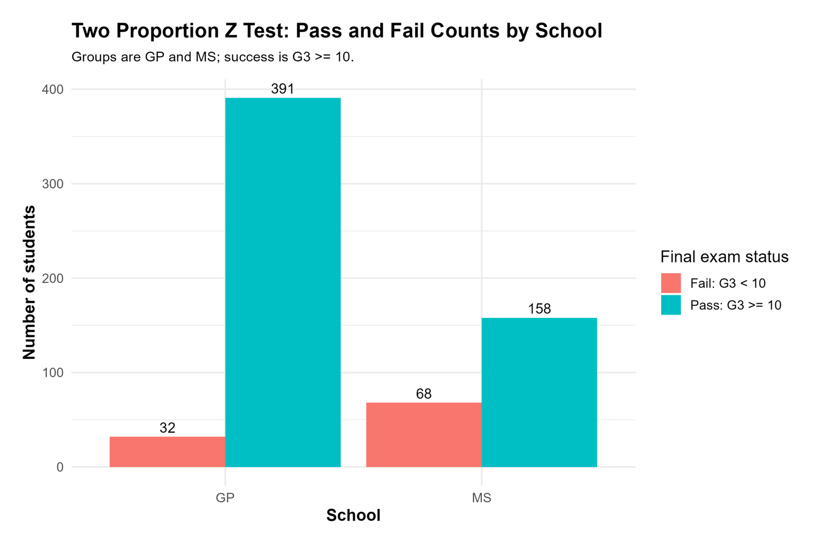
The Python count chart confirms the same values used in the SPSS output. GP has 391 passes and 32 failures. MS has 158 passes and 68 failures.
This chart is the first validation point because the z test depends on the correct count of successes and total cases in each group. The Python output matches the SPSS image, so the data coding is consistent.
The visual difference between the two schools is clear. GP has a much smaller failure share than MS, which leads to the higher GP pass proportion.
2. Python Chart: Pass Proportion Comparison by School
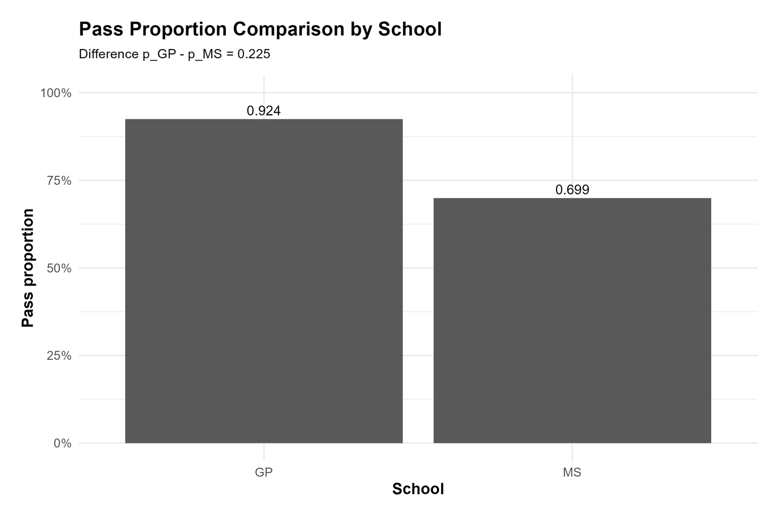
The Python proportion chart shows pGP = 0.924 and pMS = 0.699. The chart also states the difference as approximately 0.225.
This is the central visual comparison for the two sample z test for proportions. The difference between the bars is large enough to be practically meaningful and statistically meaningful.
Because Python confirms the same pass proportions as SPSS, it validates the result from an independent workflow.
3. Python Chart: Confidence Interval for Difference in Proportions
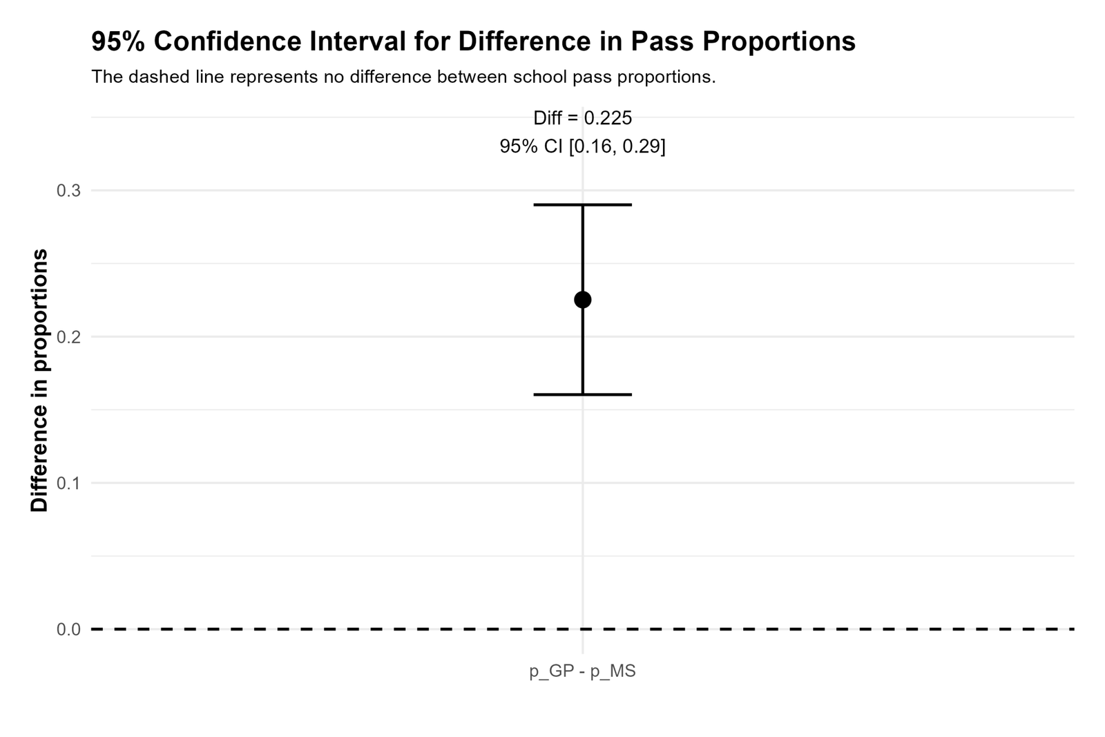
The Python confidence interval chart confirms that the estimated difference is 0.225 with a 95% confidence interval of about [0.160, 0.290].
The full interval is above zero, so the data support a positive difference between GP and MS. This means GP has a higher pass proportion than MS.
The confidence interval gives practical interpretation: the true difference is likely between 16.0 and 29.0 percentage points.
4. Python Chart: Z Statistic on the Standard Normal Curve
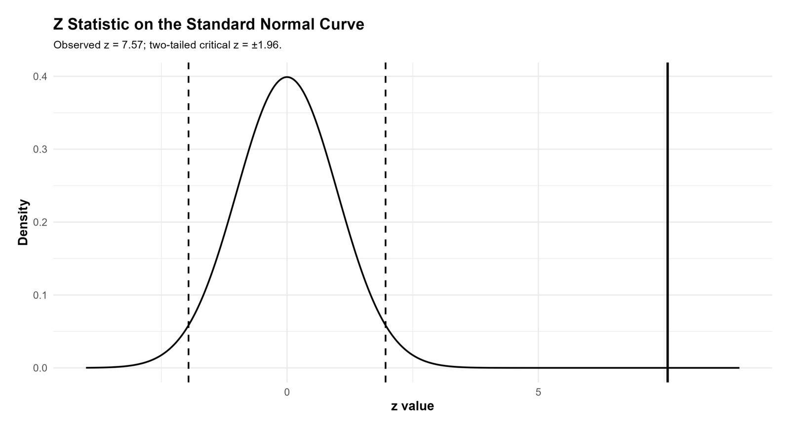
The Python standard normal curve chart shows the observed z statistic relative to the normal distribution. The observed value is z = 7.57.
This value is far beyond the ordinary two-tailed critical values of ±1.96. Therefore, the observed difference in school pass proportions is far outside the expected range under the null hypothesis of equal proportions.
The Python chart confirms the p-value decision: the result is statistically significant, and the null hypothesis should be rejected.
5. Python Chart: Pass/Fail Percentage Composition by School

The Python percentage composition chart places both schools on the same proportional scale. GP has 92.4% pass and 7.6% fail. MS has 69.9% pass and 30.1% fail.
This chart is useful for readers because it avoids confusion caused by unequal sample sizes. GP has 423 students and MS has 226 students, so percentages are easier to compare than raw counts alone.
The image confirms that MS has a much larger failure share, which explains the lower MS pass proportion.
6. Python Chart: Pass Proportion by Sex Within School
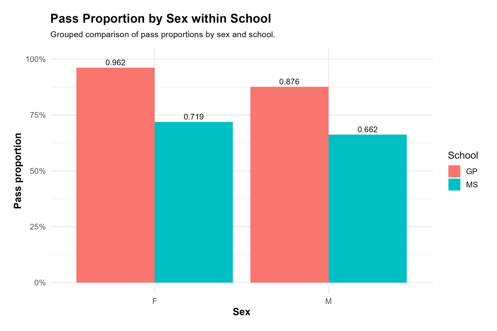
The Python sex-within-school chart shows the same subgroup pattern as SPSS. GP has higher pass proportions than MS for both female and male students. Female students: GP = 96.2%, MS = 71.9%. Male students: GP = 87.6%, MS = 66.3%.
This chart helps explain the overall school difference. The GP advantage appears within both sex categories, not only in one subgroup.
The chart is descriptive and does not replace the main two proportion z test. It helps readers understand the data pattern behind the overall school comparison.
7. Python Chart: Pass Proportion by Study Time Within School
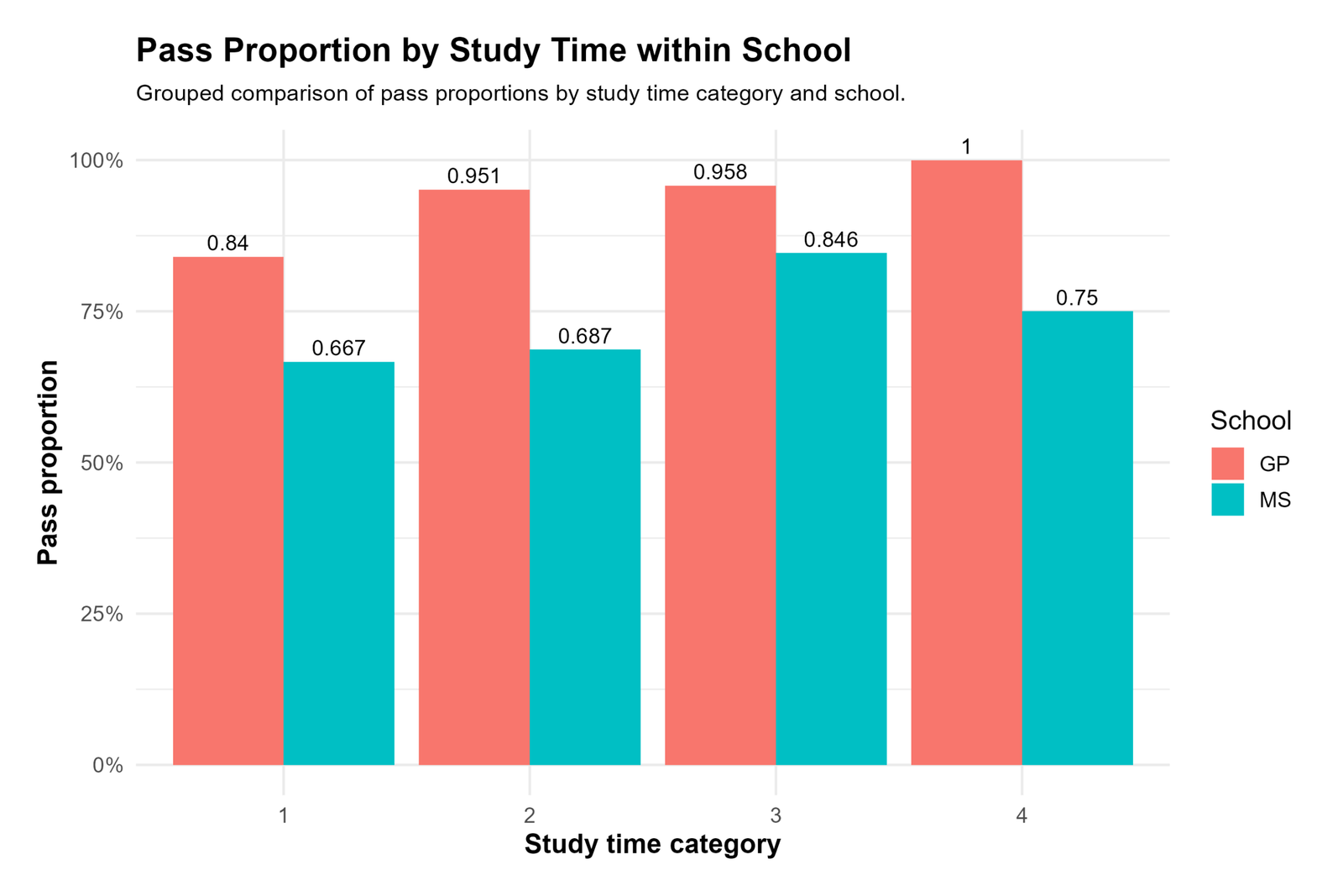
The Python study-time chart shows pass proportions for GP and MS across study-time categories 1 through 4. GP remains higher than MS in every category.
The exact values are: study time 1, GP = 84.0% and MS = 66.7%; study time 2, GP = 95.1% and MS = 68.7%; study time 3, GP = 95.8% and MS = 84.6%; study time 4, GP = 100.0% and MS = 75.0%.
This chart supports the descriptive conclusion that GP has a stronger pass proportion across study-time groups. The formal inferential conclusion still comes from the overall Two Proportion Z Test.
R Validation Charts and Interpretation
The R charts provide another independent validation of the same result. R confirms the count structure, school pass proportions, confidence interval, z statistic and subgroup patterns.
1. R Chart: Pass and Fail Counts by School
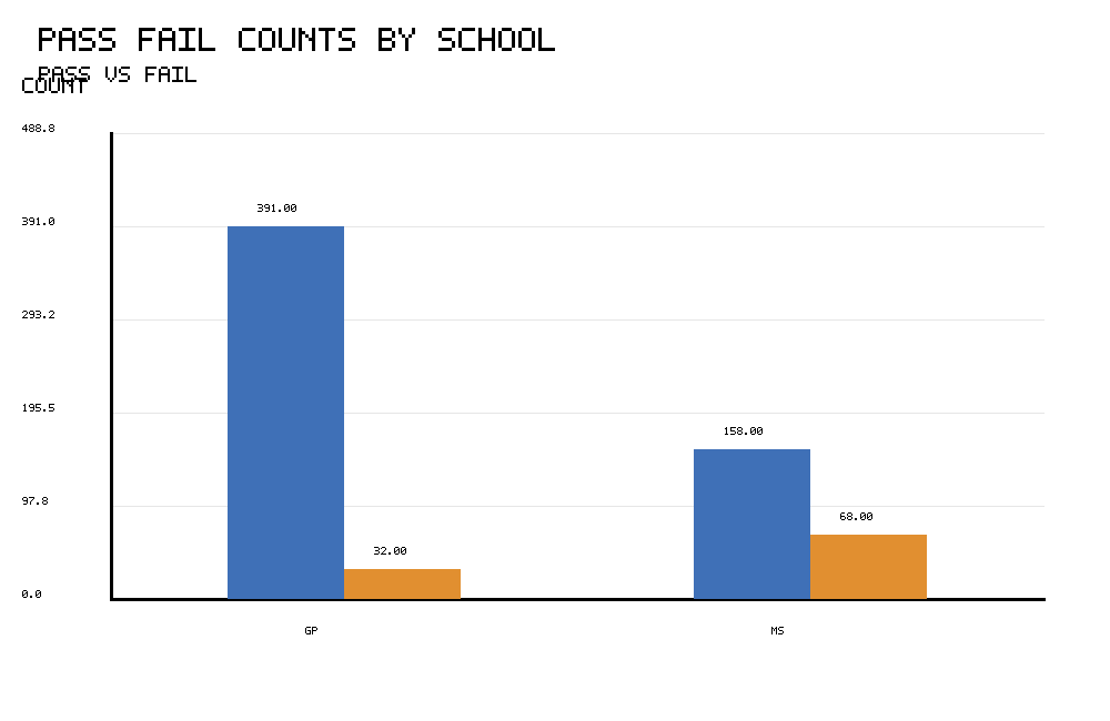
The R count chart confirms that the same data are being used across software. GP has 391 passes and 32 failures, while MS has 158 passes and 68 failures.
This verifies that the R workflow uses the same pass/fail coding as SPSS and Python. Since the counts match, the computed proportions and z statistic should also match.
The count pattern again shows the core reason for the significant result: GP has a much smaller failure share than MS.
2. R Chart: Pass Proportion Comparison by School
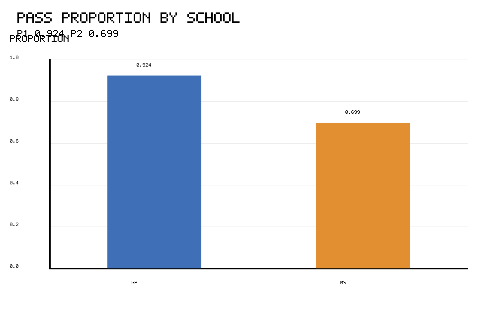
The R proportion chart confirms p1 = 0.924 for GP and p2 = 0.699 for MS. The visual difference is the same as the SPSS and Python images.
The observed difference is 0.225. This means the GP pass proportion is approximately 22.5 percentage points higher than the MS pass proportion.
Because R confirms the same values, it provides strong validation that the result is not a software-specific artifact.
3. R Chart: Confidence Interval for Difference in Proportions
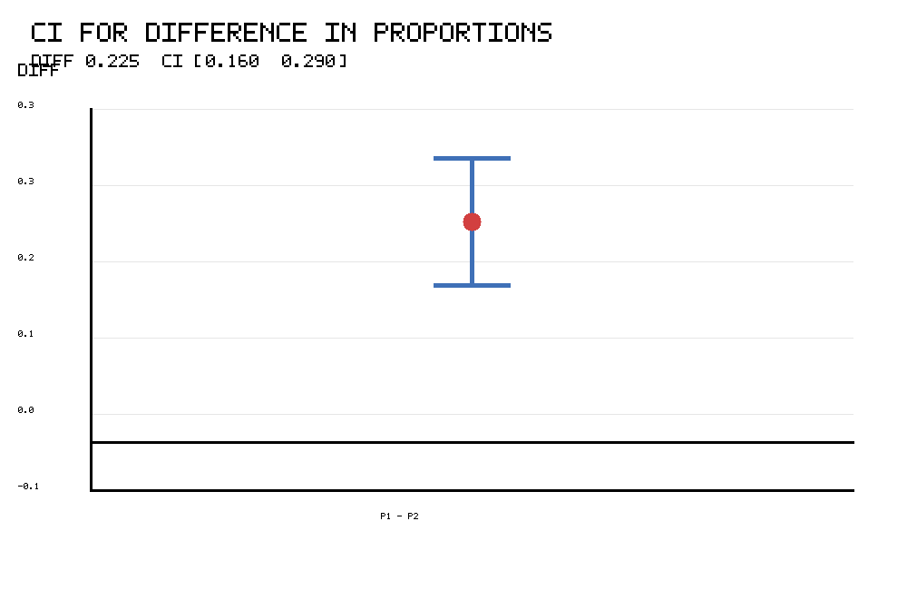
The R confidence interval chart validates the same interval estimate: [0.160, 0.290]. The point estimate is 0.225.
The interval is entirely above zero, which means the difference is positive in the estimated population. This supports the conclusion that GP has a higher pass proportion than MS.
The R chart also helps communicate the effect size. The school difference is likely not only statistically significant but also meaningful in practical terms.
4. R Chart: Z Statistic on the Standard Normal Curve
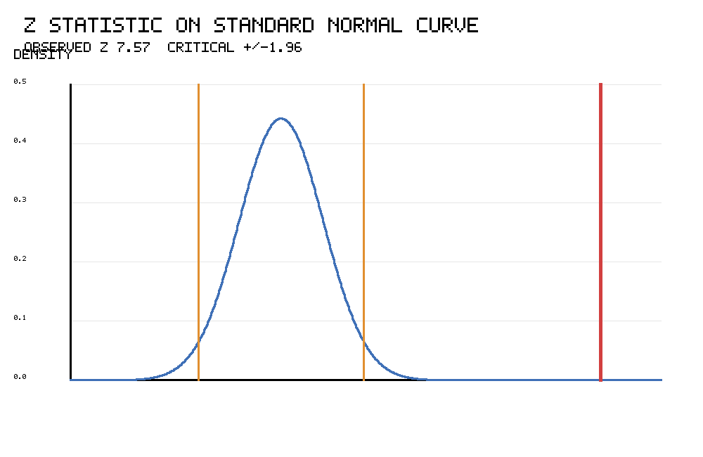
The R standard normal curve chart confirms the formal z-test decision. The observed z statistic is 7.57, far beyond the critical values of ±1.96.
A z value this extreme means the observed difference would be highly unlikely under the null hypothesis of equal pass proportions.
Therefore, the R chart supports the same final decision: reject the null hypothesis and conclude that the two school pass proportions are significantly different.
5. R Chart: Pass/Fail Percentage Composition by School

The R percentage composition image confirms the same school pattern. GP has a pass share of about 92.4%, while MS has a pass share of about 69.9%.
This chart presents the difference in an easy-to-read percentage format. It makes clear that the failure share is much larger in MS than in GP.
The percentage composition supports the test result by showing why the difference in proportions is large.
6. R Chart: Pass Proportion by Sex Within School
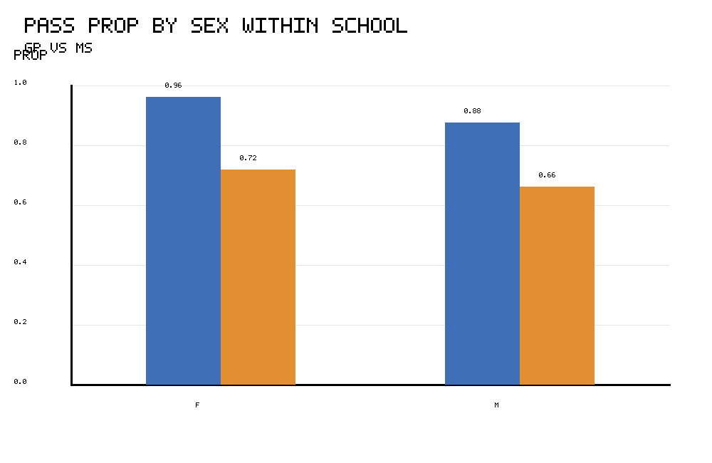
The R sex-within-school chart confirms the subgroup values. Female students have GP = 96.2% and MS = 71.9%. Male students have GP = 87.6% and MS = 66.3%.
In both sex categories, GP has a higher pass proportion than MS. This supports the descriptive interpretation that the school difference appears across sex groups.
The chart is not a replacement for the main test. It is validation and subgroup context for the overall school comparison.
7. R Chart: Pass Proportion by Study Time Within School
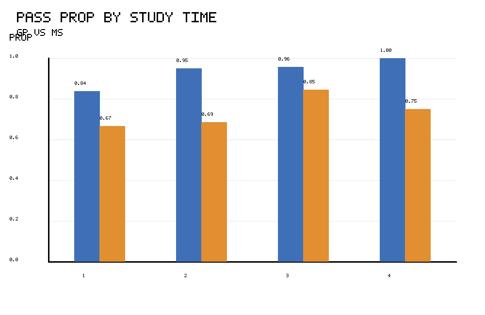
The R study-time chart confirms the same study-time pattern. GP is higher than MS in every study-time category.
The exact values are: category 1, 84.0% versus 66.7%; category 2, 95.1% versus 68.7%; category 3, 95.8% versus 84.6%; category 4, 100.0% versus 75.0%.
This chart provides useful context, but the final inferential decision remains based on the overall two-proportion z statistic.
Overall Interpretation of All SPSS, Python and R Images
All three software outputs tell the same statistical story. GP has a higher pass proportion than MS. The raw count images show 391/423 passing in GP and 158/226 passing in MS. The proportion images show 0.924 versus 0.699. The confidence interval images show that the difference is positive and does not include zero. The standard normal curve images show that z = 7.57 is far into the rejection region.
| Image type | Main message | How it supports the test |
|---|---|---|
| Pass/fail count images | GP = 391 pass, 32 fail; MS = 158 pass, 68 fail | Provides x1, n1, x2 and n2. |
| Pass proportion comparison images | GP = 0.924 and MS = 0.699 | Shows the observed group difference. |
| Confidence interval images | Difference = 0.225, 95% CI [0.160, 0.290] | Shows the difference is above zero. |
| Z curve images | Observed z = 7.57 | Shows the result is far beyond ±1.96. |
| Percentage composition images | GP pass share is 92.4%; MS pass share is 69.9% | Shows practical percentage difference. |
| Sex subgroup images | GP is higher for both female and male students | Provides descriptive subgroup support. |
| Study-time subgroup images | GP is higher in every study-time category | Provides descriptive context across study habits. |
The final decision is consistent across SPSS, Python and R: reject the null hypothesis. The pass proportions are significantly different between GP and MS, and GP has the higher pass proportion.
How to Run Two Proportion Z Test in SPSS, Python, R and Excel
SPSS Method
SPSS can calculate the required counts with crosstabulation, and the z statistic can be computed from the group counts and proportions.
* Two Proportion Z Test in SPSS.
* Success condition: pass_final = 1 if G3 >= 10.

NUMERIC pass_final (F1.0).
COMPUTE pass_final = (G3 >= 10).
VALUE LABELS pass_final
  0 'Fail: G3 < 10'
  1 'Pass: G3 >= 10'.
EXECUTE.

CROSSTABS
  /TABLES=school BY pass_final
  /CELLS=COUNT ROW COLUMN.

* After counts are known:
* GP: x1 = 391, n1 = 423
* MS: x2 = 158, n2 = 226.

COMPUTE x1 = 391.
COMPUTE n1 = 423.
COMPUTE x2 = 158.
COMPUTE n2 = 226.

COMPUTE p1 = x1 / n1.
COMPUTE p2 = x2 / n2.
COMPUTE diff = p1 - p2.
COMPUTE p_pool = (x1 + x2) / (n1 + n2).
COMPUTE se_pool = SQRT(p_pool * (1 - p_pool) * (1/n1 + 1/n2)).
COMPUTE z_value = diff / se_pool.
COMPUTE p_value_two_tailed = 2 * (1 - CDF.NORMAL(ABS(z_value), 0, 1)).
COMPUTE se_unpooled = SQRT((p1 * (1 - p1) / n1) + (p2 * (1 - p2) / n2)).
COMPUTE ci_95_low = diff - 1.96 * se_unpooled.
COMPUTE ci_95_high = diff + 1.96 * se_unpooled.
EXECUTE.
Python Method
Python can calculate the two proportion z test from the two success counts and group sample sizes.
import math

x1, n1 = 391, 423   # GP
x2, n2 = 158, 226   # MS
alpha = 0.05

p1 = x1 / n1
p2 = x2 / n2
diff = p1 - p2

p_pool = (x1 + x2) / (n1 + n2)
se_pool = math.sqrt(p_pool * (1 - p_pool) * (1/n1 + 1/n2))
z_value = diff / se_pool

p_value_two_tailed = math.erfc(abs(z_value) / math.sqrt(2))

se_unpooled = math.sqrt((p1 * (1 - p1) / n1) + (p2 * (1 - p2) / n2))
ci_low = diff - 1.96 * se_unpooled
ci_high = diff + 1.96 * se_unpooled

decision = "Reject H0" if p_value_two_tailed < alpha else "Fail to reject H0"

print("p1:", p1)
print("p2:", p2)
print("Difference:", diff)
print("Pooled p:", p_pool)
print("z:", z_value)
print("p-value:", p_value_two_tailed)
print("95% CI:", ci_low, ci_high)
print("Decision:", decision)
R Method
R can reproduce the same result using direct formulas or a proportion test workflow.
x1 <- 391
n1 <- 423
x2 <- 158
n2 <- 226
alpha <- 0.05

p1 <- x1 / n1
p2 <- x2 / n2
diff <- p1 - p2

p_pool <- (x1 + x2) / (n1 + n2)
se_pool <- sqrt(p_pool * (1 - p_pool) * (1/n1 + 1/n2))
z_value <- diff / se_pool

p_value_two_tailed <- 2 * (1 - pnorm(abs(z_value)))

se_unpooled <- sqrt((p1 * (1 - p1) / n1) + (p2 * (1 - p2) / n2))
ci_low <- diff - 1.96 * se_unpooled
ci_high <- diff + 1.96 * se_unpooled

decision <- ifelse(p_value_two_tailed < alpha, "Reject H0", "Fail to reject H0")

data.frame(
  p1 = p1,
  p2 = p2,
  difference = diff,
  pooled_p = p_pool,
  z_value = z_value,
  p_value = p_value_two_tailed,
  ci_low = ci_low,
  ci_high = ci_high,
  decision = decision
)
Excel Method
Excel can calculate the Two Proportion Z Test using basic formulas. Enter the counts in cells and use formulas for proportions, pooled p, standard error, z statistic, p-value and confidence interval.
| Excel item | Example formula | Purpose |
|---|---|---|
| GP pass proportion | =391/423 | Calculates p1. |
| MS pass proportion | =158/226 | Calculates p2. |
| Difference | =p1_cell-p2_cell | Calculates p1 − p2. |
| Pooled proportion | =(391+158)/(423+226) | Calculates pooled p under H0. |
| Pooled standard error | =SQRT(p_pool*(1-p_pool)*(1/423+1/226)) | Calculates SE for the z statistic. |
| Z statistic | =difference_cell/se_pool_cell | Calculates z. |
| Two-tailed p-value | =2*(1-NORM.S.DIST(ABS(z_cell),TRUE)) | Calculates p-value. |
| Unpooled SE for CI | =SQRT(p1*(1-p1)/423+p2*(1-p2)/226) | Calculates SE for confidence interval. |
| 95% CI lower | =difference_cell-1.96*se_unpooled_cell | Lower confidence bound. |
| 95% CI upper | =difference_cell+1.96*se_unpooled_cell | Upper confidence bound. |
How to Report the Two Proportion Z Test
A complete report should include the two groups, success definition, group counts, sample proportions, difference, z statistic, p-value, confidence interval and decision.
APA-style report: A two proportion z test was conducted to compare final exam pass proportions between GP and MS schools. Pass was defined as G3 ≥ 10. The GP pass proportion was 391/423 = .924, and the MS pass proportion was 158/226 = .699. The difference was statistically significant, z = 7.572, p < .001, 95% CI for pGP − pMS [.160, .290]. Therefore, the null hypothesis of equal pass proportions was rejected. GP had a significantly higher pass proportion than MS.
In plain language, the GP school pass rate was about 92.4%, while the MS school pass rate was about 69.9%. The difference of about 22.5 percentage points is statistically significant and practically meaningful.
Common Mistakes in Two Proportion Z Test Interpretation
1. Using a one proportion z test instead
If there are two groups, use a two proportion z test. A one proportion z test is only for comparing one sample proportion with one benchmark value.
2. Forgetting to pool for the hypothesis test
The hypothesis-test standard error uses the pooled proportion because the null hypothesis says the two population proportions are equal.
3. Using the pooled standard error for the confidence interval
The confidence interval for the difference usually uses the unpooled standard error because it estimates the actual difference between proportions.
4. Reporting p = .000
Do not write p = .000. If the p-value is extremely small, report p < .001.
5. Treating subgroup charts as formal adjusted tests
The sex and study-time charts are descriptive context. They do not replace a formal adjusted model or stratified hypothesis test.
6. Confusing two proportion z test vs chi square
For a 2 × 2 table, the two proportion z test and chi-square test of independence are closely related. The z statistic squared equals the chi-square statistic in the equivalent two-sided 2 × 2 test. For broader categorical analysis, see Cross Tabulation.
FAQs About Two Proportion Z Test
What is a Two Proportion Z Test?
A Two Proportion Z Test is a hypothesis test used to compare two independent sample proportions.
When to use Two Proportion Z Test?
Use it when the outcome is binary and you want to compare two independent groups, such as pass/fail rates for two schools.
What is the Two Proportion Z Test formula?
The formula is z = (p1 − p2) / sqrt[p pooled × (1 − p pooled) × (1/n1 + 1/n2)].
What was the result in this example?
GP had 391 passes out of 423 students, and MS had 158 passes out of 226 students. The difference was 0.225, z = 7.572, p < .001, and 95% CI [0.160, 0.290].
How do you find the p-value for Two Proportion Z Test?
After calculating the z statistic, use the standard normal distribution. For a two-tailed test, p-value = 2 × [1 − Φ(|z|)]. In this example, z = 7.572, so p < .001.
Why do we pool for the Two-Proportion Z-Test?
We pool for the hypothesis test because the null hypothesis assumes the two population proportions are equal. The pooled proportion estimates the common value under H0.
What are the conditions for Two Proportion Z Test?
The outcome must be binary, the groups must be independent, observations should be independent, and expected success/failure counts should be large enough for the normal approximation.
What is the difference between One Proportion Z Test and Two Proportion Z Test?
One Proportion Z Test compares one sample proportion with one benchmark. Two Proportion Z Test compares two sample proportions from two independent groups.
Can I do Two Proportion Z Test in Excel?
Yes. Excel can calculate p1, p2, pooled proportion, standard error, z statistic, p-value and confidence interval using ordinary formulas.
Is Two Proportion Z Test the same as chi-square?
For a 2 × 2 table, the two-sided two proportion z test is closely related to the chi-square test of independence. The z statistic squared equals the chi-square statistic for the equivalent 2 × 2 comparison.

