Normality Testing and Distribution Diagnostics
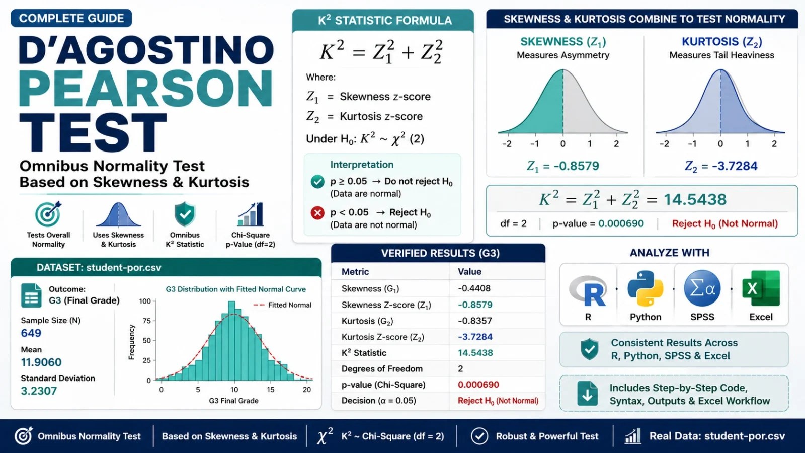
DAgostino Pearson Test is an omnibus normality test that combines skewness and kurtosis into one K2 statistic. In this guide, the test is used to check whether G3 final grades from student-por.csv follow a normal distribution. The article explains the formula, hypotheses, K2 statistic, chi-square p-value, R workflow, Python workflow, SPSS verification, Excel method, chart interpretation and verified student performance results.
Google AdSense top placement reserved here
Quick Answer: DAgostino Pearson Test Result
A DAgostino Pearson Test was conducted to evaluate whether G3 final grades follow a normal distribution. The verified result was K2 = 114.2048, with p = 1.587642e-25. The skewness was -0.9108 and the excess kurtosis was 2.6821. Since p < 0.05, the analysis rejects normality for G3 final grades.
DAgostino Pearson Test Overview
The test checks normality by looking at two important features of a distribution: skewness and kurtosis. Skewness tells whether a distribution leans left or right. Kurtosis tells whether the distribution has unusually heavy tails or a sharper/flatter shape compared with a normal distribution.
The method transforms skewness and kurtosis into two approximately standard normal z-scores. These two z-scores are then squared and added to create the K2 statistic. Under the null hypothesis of normality, K2 is compared with a chi-square distribution with 2 degrees of freedom.
In this example, the very small p-value means the G3 distribution is not normally shaped. The negative skewness and positive excess kurtosis show that the departure is caused by both asymmetry and heavy-tail/peakedness behavior.
What Is the DAgostino Pearson Test?
The D’Agostino-Pearson omnibus normality test is a formal statistical test for checking whether a sample is consistent with a normal distribution. It is called “omnibus” because it does not check only one feature. It combines skewness and kurtosis into a single overall test statistic.
In simple language: the method asks whether the distribution is too asymmetric, too heavy-tailed, too sharply peaked, or too flat to be treated as normal.
This is useful before applying statistical methods that assume normality. A histogram or Q-Q plot can show the pattern visually, but the K2 statistic gives a numerical test result.
DAgostino Pearson Test Formula
The test combines the transformed skewness and kurtosis components:
K² = Z²(skewness) + Z²(kurtosis)The p-value is calculated using a chi-square distribution with 2 degrees of freedom:
p-value = P(χ²₂ ≥ K²)For this dataset, the verified G3 result is:
K² = (-8.2817)² + (6.7542)²
K² = 114.2048
p = 1.587642e-25
The skewness z-score is strongly negative, and the kurtosis z-score is strongly positive. When squared and added, they produce a very large K2 statistic, far beyond the usual 5% chi-square critical value.
DAgostino Pearson Test Null Hypothesis and Alternative Hypothesis
| Hypothesis | Meaning | Decision rule |
|---|---|---|
| H0 | The sample comes from a normally distributed population. | If p-value is 0.05 or greater, do not reject normality. |
| H1 | The sample does not come from a normally distributed population. | If p-value is less than 0.05, reject normality. |
For G3 final grades, p is far below 0.05. Therefore, the analysis rejects the null hypothesis and concludes that the G3 distribution is not normal.
Google AdSense middle placement reserved here
Dataset and Variables Used
This example uses the student-por.csv dataset. The verified workflow uses 649 rows, 34 columns and no missing cells in the selected analysis variables. The main outcome is G3, which represents final grade. The supporting variables are G1, G2, absences and studytime.
| Variable | Role | Meaning |
|---|---|---|
| G3 | Main outcome | Final grade from 0 to 20. |
| G1 | Comparison variable | First-period grade. |
| G2 | Comparison variable | Second-period grade. |
| absences | Comparison variable | Number of school absences. |
| studytime | Group variable | Weekly study time category. |
External data source: UCI Machine Learning Repository: Student Performance dataset.
Verified DAgostino Pearson Test Results
The analysis was verified in R, Python and SPSS. R and Python produced the same K2 statistic and p-value. SPSS manually reproduced the same calculation using a clean CSV file, skewness, kurtosis, transformed z-scores, K2 statistic and chi-square p-value.
Final report sentence: A DAgostino Pearson Test was conducted to evaluate whether G3 final grades follow a normal distribution. The result was K2 = 114.2048, p = 1.587642e-25. The skewness was -0.9108 and the excess kurtosis was 2.6821. Because p < 0.05, the analysis rejected normality for G3.
Main G3 Result
| Variable | N | Mean | SD | Skewness | Excess kurtosis | K2 | p-value | Decision |
|---|---|---|---|---|---|---|---|---|
| G3 | 649 | 11.9060 | 3.2307 | -0.9108 | 2.6821 | 114.2048 | 1.587642e-25 | Reject normality |
Component Z-Scores
| Component | Z-score | Meaning |
|---|---|---|
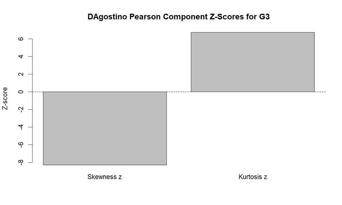
| Skewness z | -8.2817 | The negative sign shows a strong left-skewed pattern in G3. |
| Kurtosis z | 6.7542 | The positive value shows strong kurtosis departure from normality. |
Variable Comparison Results
| Variable | N | Mean | SD | Skewness | Excess kurtosis | K2 | p-value | Decision |
|---|---|---|---|---|---|---|---|---|
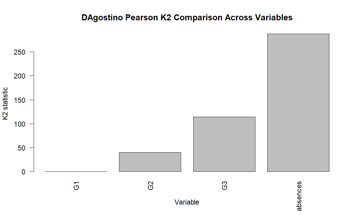
| G1 | 649 | 11.3991 | 2.7453 | -0.0028 | 0.0271 | 0.0802 | 0.9607 | Do not reject normality |
| G2 | 649 | 11.5701 | 2.9136 | -0.3594 | 1.6405 | 40.1870 | 1.877145e-09 | Reject normality |
| G3 | 649 | 11.9060 | 3.2307 | -0.9108 | 2.6821 | 114.2048 | 1.587642e-25 | Reject normality |
| absences | 649 | 3.6595 | 4.6408 | 2.0160 | 5.7274 | 287.7460 | 3.286672e-63 | Reject normality |
G3 by Studytime Group
| Studytime group | N | Mean G3 | SD | Skewness | Excess kurtosis | K2 | p-value | Decision |
|---|---|---|---|---|---|---|---|---|
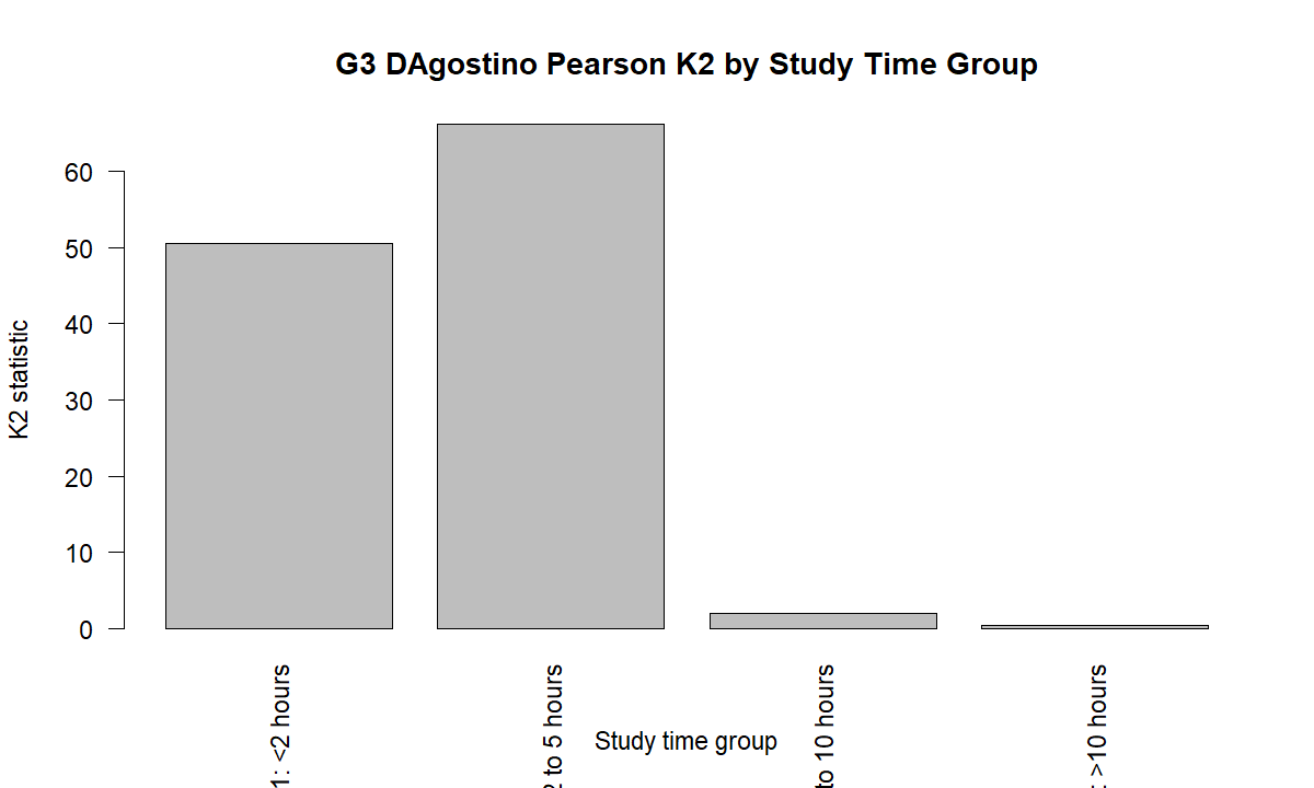
| 1: <2 hours | 212 | 10.8443 | 3.2186 | -1.0705 | 3.0162 | 50.5457 | 1.057158e-11 | Reject normality |
| 2: 2 to 5 hours | 305 | 12.0918 | 3.2431 | -1.0230 | 2.9751 | 66.2103 | 4.193909e-15 | Reject normality |
| 3: 5 to 10 hours | 97 | 13.2268 | 2.5021 | -0.1872 | -0.5374 | 2.0646 | 0.3562 | Do not reject normality |
| 4: >10 hours | 35 | 13.0571 | 3.0384 | 0.2002 | -0.4590 | 0.3974 | 0.8198 | Do not reject normality |
DAgostino Pearson Test Result Images and Chart Interpretation
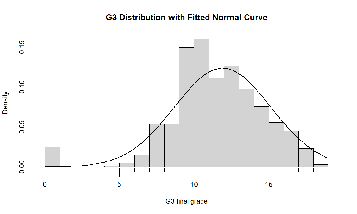
1. Histogram with Fitted Normal Curve
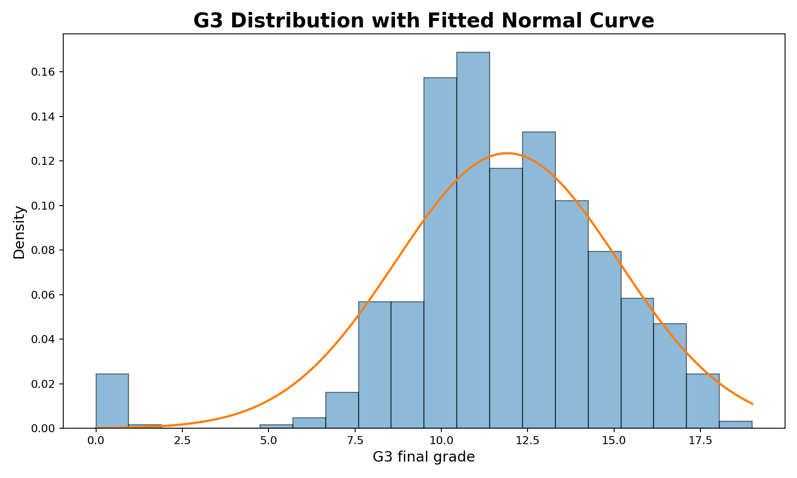
This chart shows why the normality result is not surprising. The distribution is not a smooth bell shape. G3 grades are bounded between 0 and 20, measured as integer scores, and contain a visible group of low scores near zero. The fitted normal curve cannot fully match this shape.
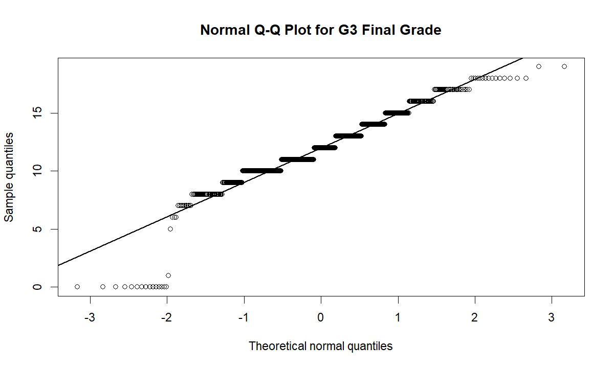
2. Normal Q-Q Plot
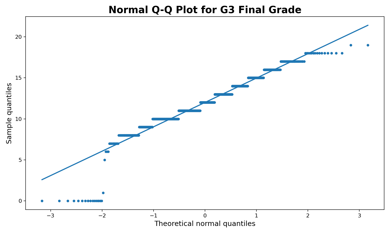
The Q-Q plot compares observed grade quantiles with theoretical normal quantiles. If G3 were normally distributed, the points would follow the reference line more closely. Instead, the plot shows stair-step behavior from repeated integer grades, a strong lower-tail departure and a high-end flattening. This visual pattern supports the formal rejection of normality.
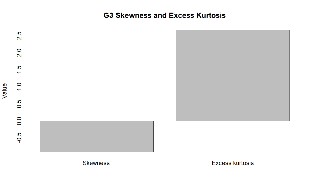
3. Skewness and Excess Kurtosis
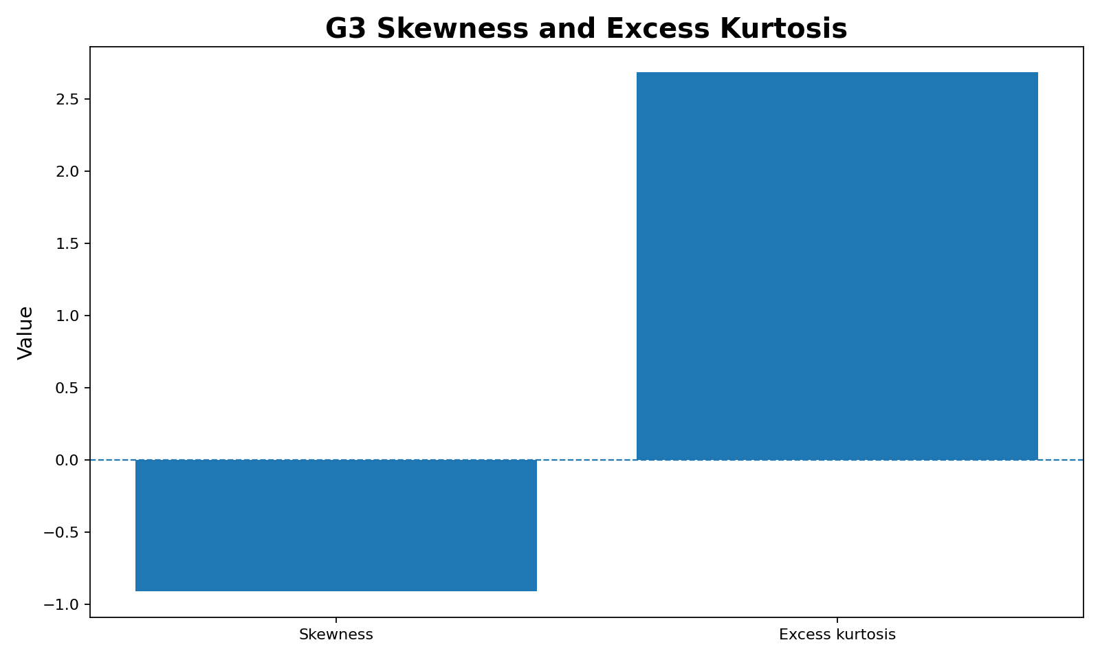
This chart shows the two shape features used by the test. G3 has negative skewness of about -0.9108, meaning the distribution has a longer or stronger lower-side pull. It also has excess kurtosis of about 2.6821, meaning the distribution departs strongly from the kurtosis expected under normality.
4. Component Z-Scores
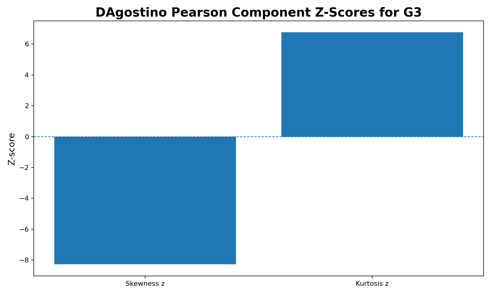
This chart explains the K2 statistic. The skewness component is strongly negative, with z ≈ -8.2817. The kurtosis component is strongly positive, with z ≈ 6.7542. The test squares both values, so both components strongly increase K2. This is why the final statistic becomes very large.
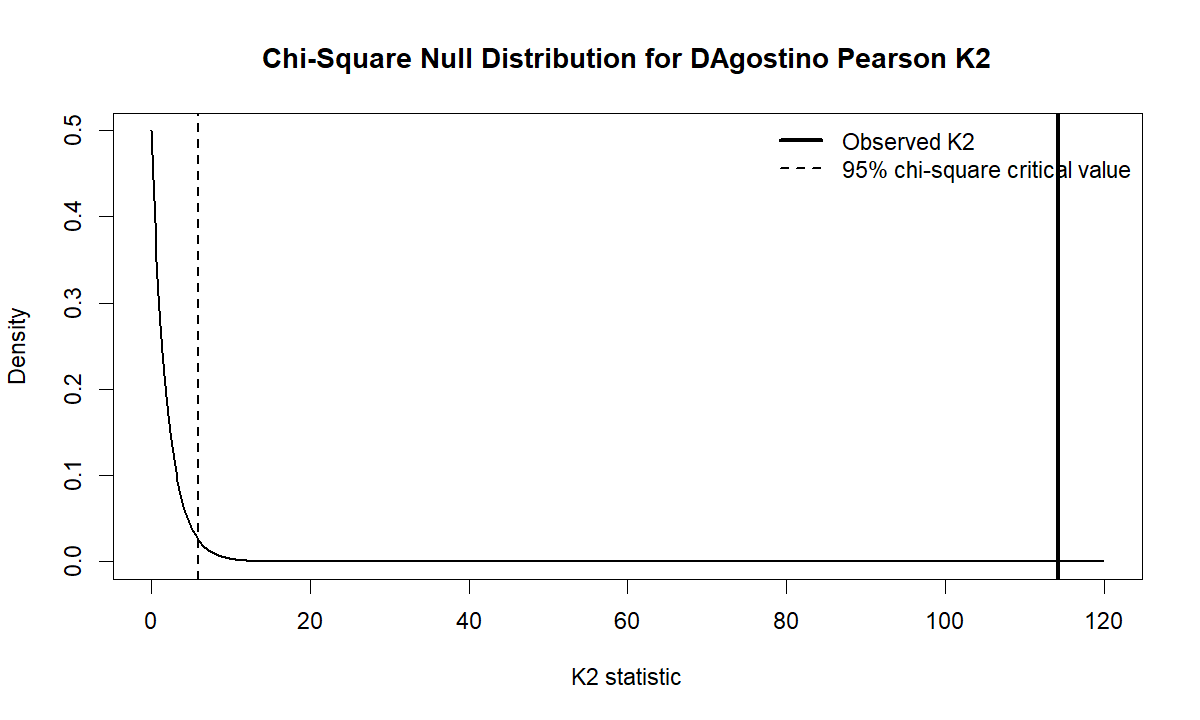
5. Chi-Square Null Distribution for K2
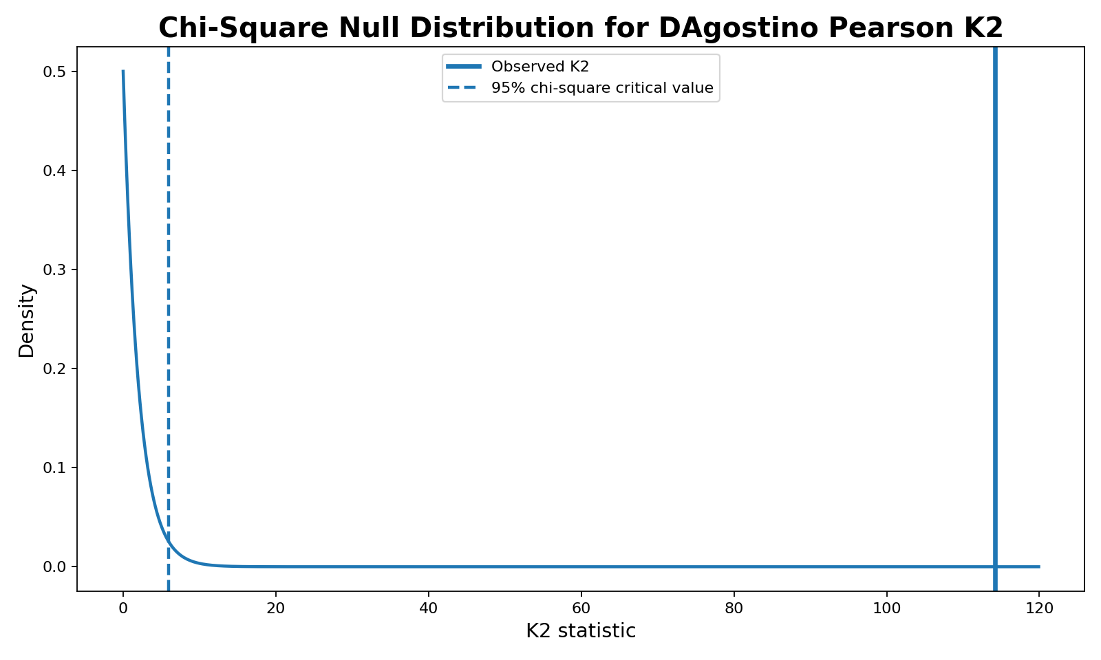
This chart shows the decision visually. The dashed line marks the 95% chi-square critical value, while the observed K2 statistic is far to the right. Since K2 = 114.2048 is much larger than the critical value, the p-value becomes extremely small and the normality assumption is rejected.
6. K2 Comparison Across Variables
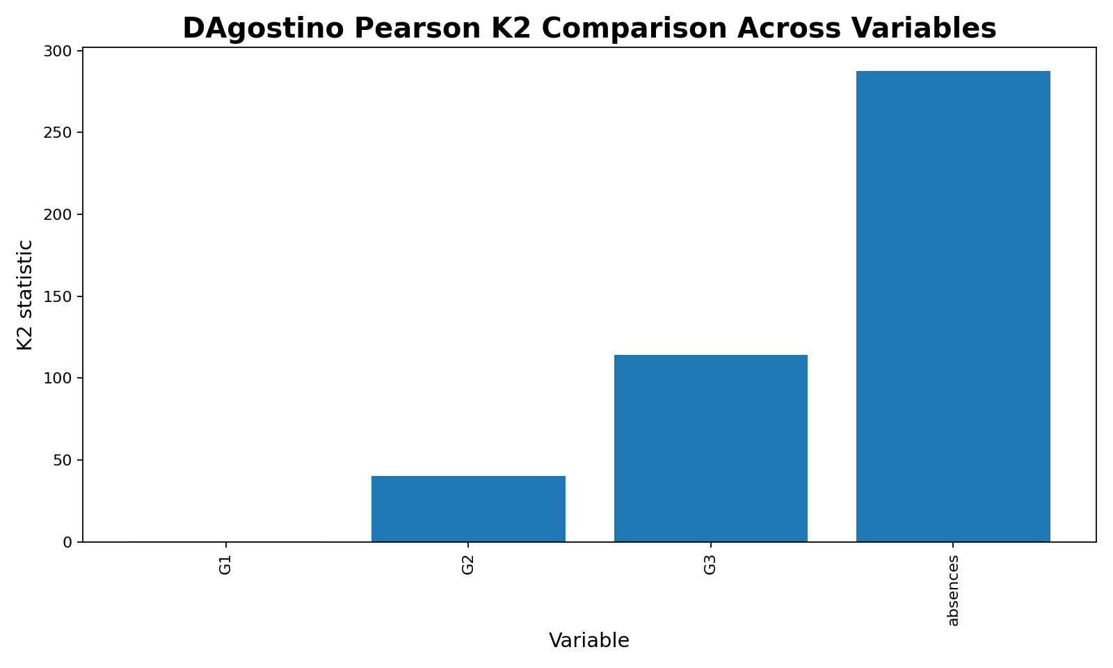
This chart compares normality departure across four variables. G1 has a very small K2 value and does not reject normality. G2 and G3 reject normality, while absences has the largest K2 value because absences are count data and are strongly non-normal. This chart helps readers understand that normality can differ across variables inside the same dataset.
7. G3 K2 by Studytime Group
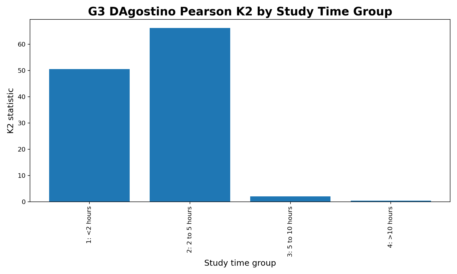
This chart shows that G3 normality differs across studytime categories. The first two groups, <2 hours and 2 to 5 hours, have large K2 values and reject normality. The 5 to 10 hours and >10 hours groups have smaller K2 values and do not reject normality at the 0.05 level. This means the overall G3 normality rejection is mainly driven by the larger lower-studytime groups.
Additional Verification Images
The “-1” image files below are duplicate verification charts from the repeated workflow. They are included for completeness. For better page speed, the seven main charts above are usually enough for the published article, while the repeated charts can remain in the media library as backup evidence.
DAgostino Pearson Test in R
In R, the test can be calculated by computing skewness, kurtosis, component transformations, K2 and the chi-square p-value.
student <- read.csv("student-por.csv", sep = ";", stringsAsFactors = FALSE)

g3 <- as.numeric(student$G3)
g3 <- g3[!is.na(g3)]

n <- length(g3)
mu <- mean(g3)
s <- sd(g3)

m2 <- mean((g3 - mu)^2)
m3 <- mean((g3 - mu)^3)
m4 <- mean((g3 - mu)^4)

skewness <- m3 / (m2^(3/2))
pearson_kurtosis <- m4 / (m2^2)
excess_kurtosis <- pearson_kurtosis - 3

# In the full workflow, skewness and kurtosis are transformed
# into z-scores, then combined:
K2 <- z_skewness^2 + z_kurtosis^2
p_value <- pchisq(K2, df = 2, lower.tail = FALSE)
The verified R output gives K2 = 114.2048 and p = 1.587642e-25.
DAgostino Pearson Test in Python
Python can reproduce the same result by calculating skewness, kurtosis, component z-scores and K2.
import pandas as pd
import numpy as np
import math

student = pd.read_csv("student-por.csv", sep=";")

g3 = pd.to_numeric(student["G3"], errors="coerce").dropna().to_numpy()

n = len(g3)
mean = np.mean(g3)
sd = np.std(g3, ddof=1)

m2 = np.mean((g3 - mean) ** 2)
m3 = np.mean((g3 - mean) ** 3)
m4 = np.mean((g3 - mean) ** 4)

skewness = m3 / (m2 ** 1.5)
pearson_kurtosis = m4 / (m2 ** 2)
excess_kurtosis = pearson_kurtosis - 3

# After D'Agostino-Pearson transformations:
K2 = z_skewness ** 2 + z_kurtosis ** 2
p_value = math.exp(-K2 / 2)  # chi-square df = 2 survival function

print(K2, p_value)
The verified Python result matches R and SPSS: K2 = 114.204755, p = 1.587642e-25.
DAgostino Pearson Test in SPSS
SPSS can manually verify the calculation by importing a clean CSV file, computing central moments, transforming skewness and kurtosis into z-scores, and calculating the K2 statistic.
SPSS Manual G3 Result
| N | Mean G3 | SD G3 | Skewness | Excess kurtosis | Skewness z | Kurtosis z | K2 | p-value | Decision |
|---|---|---|---|---|---|---|---|---|---|
| 649 | 11.906009 | 3.230656 | -0.910798 | 2.682123 | -8.281651 | 6.754184 | 114.204755 | 1.58764160E-25 | Reject normality |
SPSS Syntax Used
GET DATA
  /TYPE=TXT
  /FILE='D:\dagostino_pearson_test\student_dap_spss_clean.csv'
  /ENCODING='UTF8'
  /DELIMITERS=","
  /QUALIFIER='"'
  /FIRSTCASE=2
  /VARIABLES=
  studytime F1.0
  G1 F2.0
  G2 F2.0
  G3 F2.0
  absences F3.0.
CACHE.
EXECUTE.

AGGREGATE
  /OUTFILE=* MODE=ADDVARIABLES
  /BREAK=
  /n_total=N(G3)
  /mean_G3=MEAN(G3)
  /sd_G3=SD(G3).

COMPUTE dev_G3 = G3 - mean_G3.
COMPUTE dev2_G3 = dev_G3 ** 2.
COMPUTE dev3_G3 = dev_G3 ** 3.
COMPUTE dev4_G3 = dev_G3 ** 4.
EXECUTE.

AGGREGATE
  /OUTFILE=* MODE=ADDVARIABLES
  /BREAK=
  /m2_G3=MEAN(dev2_G3)
  /m3_G3=MEAN(dev3_G3)
  /m4_G3=MEAN(dev4_G3).

COMPUTE skewness_G3 = m3_G3 / (m2_G3 ** 1.5).
COMPUTE pearson_kurtosis_G3 = m4_G3 / (m2_G3 ** 2).
COMPUTE excess_kurtosis_G3 = pearson_kurtosis_G3 - 3.

COMPUTE K2_G3 = (z_skewness_G3 ** 2) + (z_kurtosis_G3 ** 2).
COMPUTE p_value_G3 = EXP(-K2_G3 / 2).
EXECUTE.
Download SPSS verification PDF: DAgostino Pearson Test SPSS Output PDF.
DAgostino Pearson Test in Excel
Excel can calculate skewness and kurtosis, but the full transformed K2 calculation is easier in R or Python. Still, Excel is useful for understanding the logic.
- Place G3 values in one column.
- Calculate sample size, mean and standard deviation.
- Calculate skewness.
- Calculate kurtosis or excess kurtosis.
- Transform skewness and kurtosis into z-scores using the formula.
- Square both z-scores and add them to get K2.
- Use the chi-square distribution with 2 degrees of freedom to calculate the p-value.
=SKEW(G3_range)
=KURT(G3_range)
=Z_skewness^2 + Z_kurtosis^2
=CHISQ.DIST.RT(K2, 2)
How to Report the DAgostino Pearson Test
A strong report should include the variable, sample size, skewness, excess kurtosis, K2 statistic, p-value and final decision.
APA-style report: A DAgostino Pearson Test was conducted to evaluate whether G3 final grades followed a normal distribution. The result was K2 = 114.2048, p = 1.587642e-25. The distribution showed negative skewness of -0.9108 and excess kurtosis of 2.6821. Since p < 0.05, the normality assumption was rejected.
Plain-language report: G3 final grades are not normally distributed. The distribution is left-skewed and has strong kurtosis departure, so a normal curve does not describe the grade pattern well.
Common Mistakes in DAgostino Pearson Test
1. Reporting only the p-value
The p-value is important, but a complete interpretation should also mention skewness, kurtosis and K2.
2. Ignoring the direction of skewness
A significant result tells you normality is rejected, but skewness tells whether the departure is left-sided or right-sided.
3. Treating K2 as variance
K2 is not variance. It is the sum of squared skewness and kurtosis z-scores.
4. Using the test without visual charts
A histogram and Q-Q plot help explain why normality is rejected.
5. Using it for very small samples
The method is generally more useful with moderate or large samples. For very small samples, normality tests can be unstable.
Download DAgostino Pearson Test Files
The SPSS PDF contains the verified manual output, including import checks, G3 result, variable comparison and studytime-group comparison.
Sources and Method Notes
This guide uses verified R, Python and SPSS outputs from the student performance dataset. The following sources support the dataset and software environment.
FAQs About DAgostino Pearson Test
What is the DAgostino Pearson Test?
It is an omnibus normality test that combines skewness and kurtosis into one K2 statistic.
What does K2 mean?
K2 is the sum of the squared skewness z-score and squared kurtosis z-score. A large K2 value indicates stronger departure from normality.
What was the result in this example?
The result for G3 was K2 = 114.2048 with p = 1.587642e-25, so normality was rejected.
What do skewness and kurtosis show here?
G3 has negative skewness of about -0.9108 and excess kurtosis of about 2.6821, indicating strong departure from a normal shape.
Can this test be run in R?
Yes. R can calculate skewness, kurtosis, transformed z-scores, K2 and the chi-square p-value.
Can this test be run in Python?
Yes. Python can reproduce the same calculation using pandas, numpy and the chi-square p-value formula.
Can this test be run in SPSS?
Yes. SPSS can manually calculate the test using central moments, skewness, kurtosis, component transformations and K2.
Can this test be run in Excel?
Excel can calculate skewness and kurtosis, but R or Python is better for the full transformed K2 workflow.
Google AdSense bottom placement reserved here