
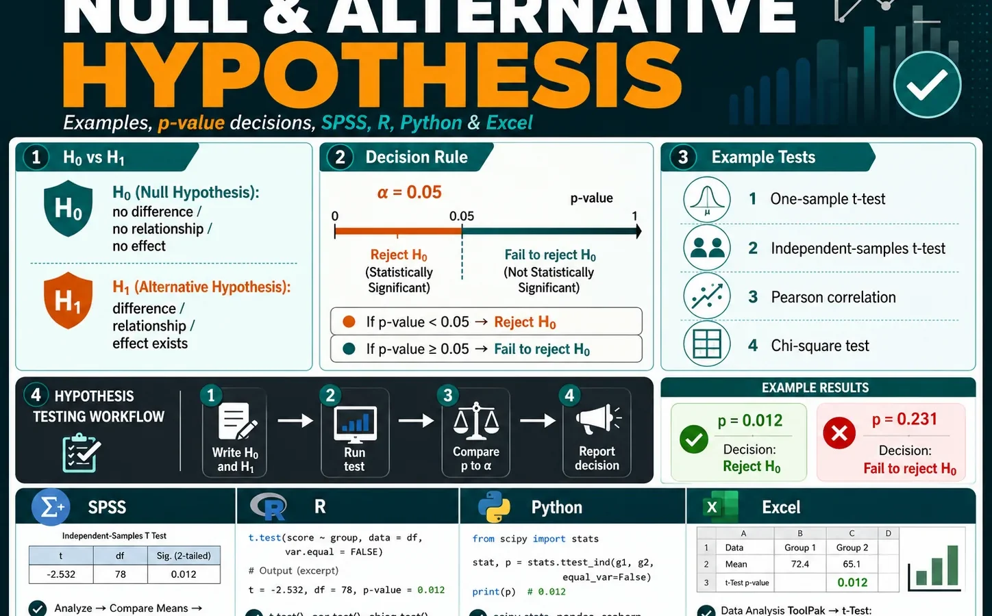
Hypothesis Testing, p-value Decisions, SPSS, R, Python and Excel
Null and alternative hypothesis statements are the foundation of statistical testing. The null hypothesis usually says that there is no difference, no relationship, no association, or no effect. The alternative hypothesis says that a difference, relationship, association, or effect exists. This guide explains how to write hypotheses, how to compare the p-value with alpha = 0.05, and how to report one-sample, two-group, correlation, and chi-square hypothesis examples using SPSS, Python, R and Excel.
Quick Answer: What Are Null and Alternative Hypotheses?
The null hypothesis, written as H0, is the default claim tested by a statistical test. It usually states that there is no difference, no relationship, no association, or no effect. The alternative hypothesis, written as H1 or Ha, is the research claim. It states that a meaningful difference, relationship, association, or effect exists.
The decision rule is simple: compare the p-value with the significance level, usually alpha = 0.05. If the p-value is less than 0.05, reject the null hypothesis. If the p-value is greater than or equal to 0.05, fail to reject the null hypothesis. In the verified SPSS examples for this guide, all four example tests have p-values below 0.05, so all four examples lead to reject the null hypothesis.
Main result: The one-sample t-test, independent-samples t-test, Pearson correlation test, and chi-square independence test all show statistically significant results at alpha = 0.05. Therefore, the null hypothesis is rejected in each example.
Table of Contents
- What Null and Alternative Hypothesis Mean
- Null and Alternative Hypothesis Symbols
- p-value Decision Rule
- Dataset and Variables Used
- Verified SPSS Results
- Chart-by-Chart Interpretation
- How to Test Hypotheses in Python, R, SPSS and Excel
- How to Report Null and Alternative Hypothesis Results
- Common Mistakes
- Download SPSS Output
- FAQs
What Null and Alternative Hypothesis Mean
A hypothesis is a formal statistical statement about a population parameter. In a data analysis report, the hypothesis tells readers exactly what is being tested. Without the null and alternative hypothesis, a p-value has no clear meaning because the reader does not know what claim the test is evaluating.
The null hypothesis is the starting assumption. For example, in a one-sample mean test, the null hypothesis may say that the population mean equals a benchmark value. In a two-group mean test, the null hypothesis may say that two population means are equal. In a correlation test, the null hypothesis may say that the population correlation is zero. In a chi-square test, the null hypothesis may say that two categorical variables are independent.
The alternative hypothesis is the competing statement. It represents the pattern that the researcher is trying to support with evidence. If the data produce a small p-value, the result is unlikely under the null hypothesis, so we reject the null hypothesis and interpret the alternative hypothesis as supported by the sample evidence.
Simple meaning: H0 says “nothing special is happening.” H1 says “something is happening.” The p-value helps decide whether the sample evidence is strong enough to reject H0.
Null and Alternative Hypothesis Symbols
The most common symbols are H0 for the null hypothesis and H1 or Ha for the alternative hypothesis. The exact symbol depends on the test.
| Test type | Null hypothesis | Alternative hypothesis | Plain meaning |
|---|---|---|---|
| One-sample mean test | H0: μ = 10 | H1: μ ≠ 10 | The population mean is compared with a benchmark value. |
| Independent-samples t-test | H0: μfemale = μmale | H1: μfemale ≠ μmale | The two group means are compared. |
| Pearson correlation test | H0: ρ = 0 | H1: ρ ≠ 0 | The population correlation is tested against zero. |
| Chi-square independence test | H0: variables are independent | H1: variables are associated | Two categorical variables are tested for association. |
For broader test selection, related examples include one-tailed t-test, one-sample z-test, one-proportion z-test, cross tabulation, and effect size.
p-value Decision Rule for Null and Alternative Hypothesis
The p-value is the probability of getting a result at least as extreme as the sample result if the null hypothesis were true. A small p-value means the observed result is unlikely under H0. The usual decision rule at alpha = 0.05 is:
| Condition | Decision | Correct wording |
|---|---|---|
| p-value < 0.05 | Reject H0 | There is statistically significant evidence for the alternative hypothesis. |
| p-value ≥ 0.05 | Fail to reject H0 | There is not enough statistical evidence for the alternative hypothesis. |
Important reporting rule: Do not say “accept the null hypothesis” unless the test was specifically designed for equivalence or non-inferiority. In most ordinary hypothesis tests, the correct wording is fail to reject the null hypothesis.
Dataset and Variables Used
The worked examples use the student performance dataset with 649 valid cases. The main outcome is G3 final grade. The examples use G3 for a one-sample mean test, G3 by sex for a two-group mean test, G2 and G3 for a Pearson correlation test, and school by higher education intention for a chi-square independence test.
| Variable | SPSS label | N | Minimum | Maximum | Mean | SD |
|---|---|---|---|---|---|---|
| G1 | First period grade | 649 | 0 | 19 | 11.40 | 2.745 |
| G2 | Second period grade | 649 | 0 | 19 | 11.57 | 2.914 |
| G3 | Final grade | 649 | 0 | 19 | 11.91 | 3.231 |
| absences | School absences | 649 | 0 | 32 | 3.66 | 4.641 |
| age | Student age | 649 | 15 | 22 | 16.74 | 1.218 |
The same dataset is often used in related descriptive and assumption guides such as descriptive statistics, frequency distribution, five-number summary, box plot interpretation, and histogram interpretation.
Verified SPSS Results for Hypothesis Testing
Example 1: One-Sample t-Test for G3
Null hypothesis: H0: Mean G3 = 10. Alternative hypothesis: H1: Mean G3 is different from 10.
| Statistic | SPSS value | Interpretation |
|---|---|---|
| N | 649 | There are 649 valid G3 scores. |
| Sample mean | 11.91 | The observed mean is above the benchmark of 10. |
| Standard deviation | 3.231 | Spread of G3 scores. |
| Standard error | .127 | Estimated sampling error of the mean. |
| t | 15.030 | The sample mean is far from the benchmark in standard error units. |
| df | 648 | Degrees of freedom for the one-sample t-test. |
| Sig. (2-tailed) | .000 | Report as p < .001. |
| Mean difference | 1.906 | G3 mean is about 1.91 points higher than 10. |
| 95% CI of difference | 1.66 to 2.16 | The entire interval is above zero, supporting rejection of H0. |
Hypothesis decision: Since p < .001, reject the null hypothesis. The sample mean G3 is significantly different from 10, and the direction of the result shows that the mean is significantly higher than 10.
Example 2: Independent-Samples t-Test for G3 by Sex
Null hypothesis: H0: Mean G3 is equal for female and male students. Alternative hypothesis: H1: Mean G3 differs between female and male students.
| Group | N | Mean | SD | SE | Interpretation |
|---|---|---|---|---|---|
| Female | 383 | 12.25 | 3.124 | .160 | Female students have the higher mean G3 score. |
| Male | 266 | 11.41 | 3.321 | .204 | Male students have a lower mean G3 score. |
| Test component | SPSS value | Interpretation |
|---|---|---|
| Levene’s test F | .004 | Variance equality test statistic. |
| Levene’s Sig. | .950 | Variances are not significantly different, so the equal variances assumed row is appropriate. |
| t | 3.311 | Mean difference is statistically large enough relative to its standard error. |
| df | 647 | Degrees of freedom for equal variances assumed. |
| Sig. (2-tailed) | .001 | p-value is below .05. |
| Mean difference | .847 | Female mean is about .85 grade points higher than male mean. |
| 95% CI | .345 to 1.350 | The interval is entirely above zero, supporting a significant difference. |
Hypothesis decision: Since p = .001, reject the null hypothesis. The G3 final grade differs significantly by sex group. The female mean is higher than the male mean in this sample. For a deeper check of the variance assumption used before reading the equal-variance t-test row, see Levene test and Brown-Forsythe test.
Example 3: Pearson Correlation Hypothesis Test for G2 and G3
Null hypothesis: H0: The population correlation between G2 and G3 is zero. Alternative hypothesis: H1: The population correlation between G2 and G3 is not zero.
| Statistic | SPSS value | Interpretation |
|---|---|---|
| Pearson correlation | .919 | Very strong positive relationship between G2 and G3. |
| Sig. (2-tailed) | .000 | Report as p < .001. |
| N | 649 | Correlation is based on 649 valid pairs. |
Hypothesis decision: Since p < .001, reject the null hypothesis. G2 and G3 have a statistically significant positive correlation. In practical terms, students with higher second-period grades tend to have higher final grades.
Example 4: Chi-Square Independence Test for School and Higher Education Intention
Null hypothesis: H0: School and higher education intention are independent. Alternative hypothesis: H1: School and higher education intention are associated.
| School | Higher = no | Higher = yes | Total | % yes within school |
|---|---|---|---|---|
| GP | 32 | 391 | 423 | 92.4% |
| MS | 37 | 189 | 226 | 83.6% |
| Total | 69 | 580 | 649 | 89.4% |
| Statistic | SPSS value | Interpretation |
|---|---|---|
| Pearson chi-square | 12.024 | Difference between observed and expected counts. |
| df | 1 | Degrees of freedom for the 2 × 2 table. |
| Asymptotic Sig. | .001 | p-value is below .05. |
| Minimum expected count | 24.03 | Expected count assumption is satisfied. |
| Cramer’s V | .136 | Small association size. |
Hypothesis decision: Since p = .001, reject the null hypothesis. School and higher education intention are not independent in this sample. The association is statistically significant, but the effect size is small because Cramer’s V is .136. For more on crosstab tables and association measures, see cross tabulation and effect size.
Chart-by-Chart Interpretation
Python Chart 1: Null vs Alternative Hypothesis p-value Decisions
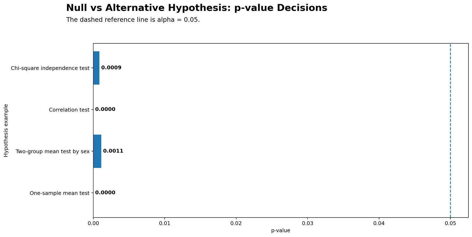
This chart summarizes the hypothesis decision rule visually. The horizontal axis is the p-value, and the dashed vertical reference line marks alpha = 0.05. Each horizontal bar represents one hypothesis test example. The one-sample mean test and correlation test appear at or near 0.0000 because their p-values are extremely small. This does not mean the p-value is literally zero; it means the p-value is smaller than the displayed rounding level and should be reported as p < .001. The two-group mean test by sex has a p-value around 0.0011, and the chi-square independence test has a p-value around 0.0009. All four bars are far to the left of the 0.05 reference line. Therefore, every test produces the same decision: reject the null hypothesis. The chart is useful because it shows that the conclusion is not borderline. The p-values are not just slightly below 0.05; they are much smaller than alpha, so the evidence against H0 is strong in each example.
Python Chart 2: One-Sample Hypothesis Example for G3
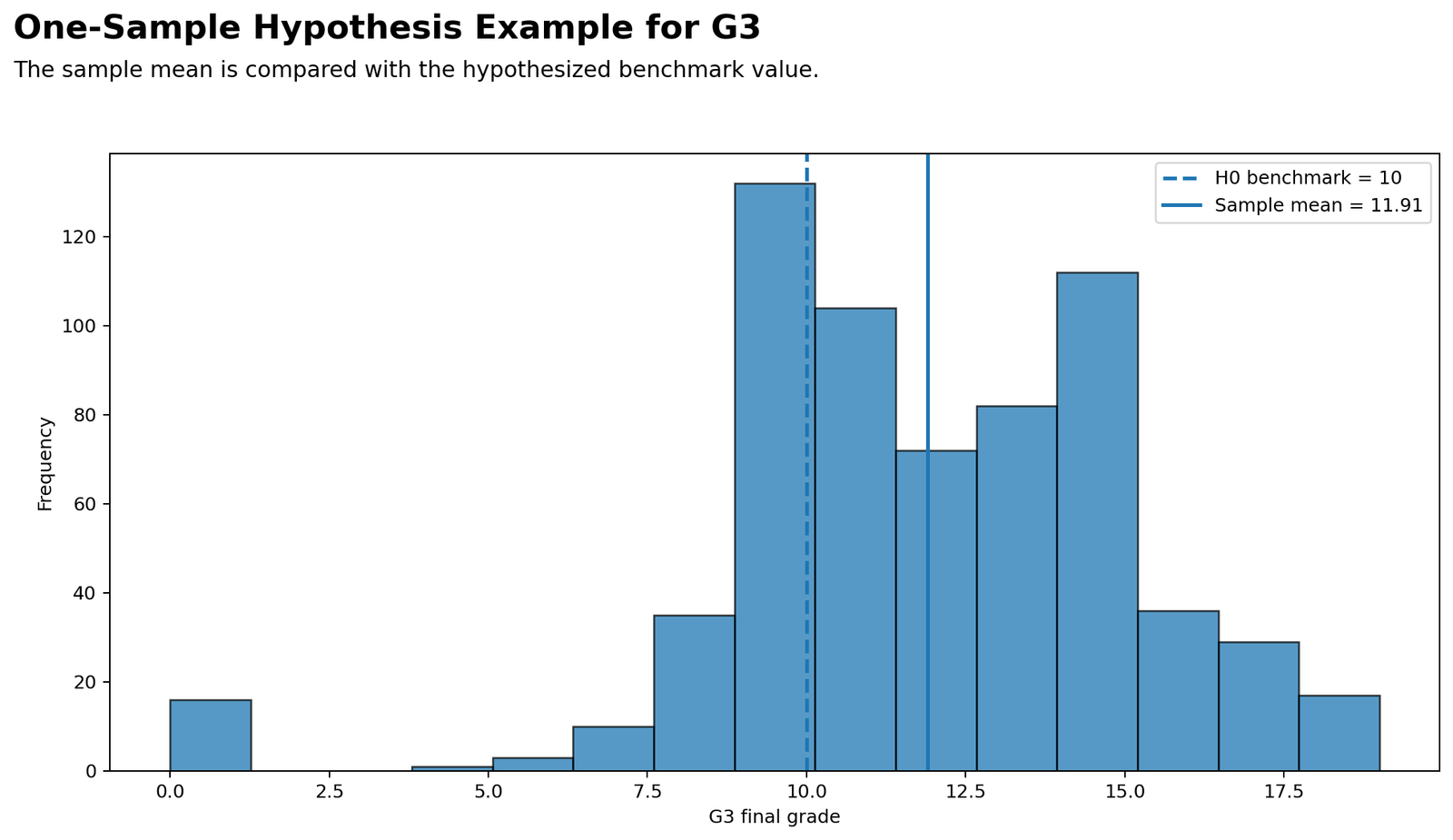
This chart explains the one-sample hypothesis test. The histogram shows the distribution of G3 final grade. The dashed vertical line is the null-hypothesis benchmark, H0 benchmark = 10. The solid vertical line is the observed sample mean, sample mean = 11.91. Since the sample mean is clearly to the right of the benchmark, the observed average final grade is higher than the value stated in the null hypothesis. SPSS confirms this visual difference with t(648) = 15.030, p < .001, a mean difference of 1.906, and a 95% confidence interval from 1.66 to 2.16. The confidence interval does not include zero, so the result supports rejecting H0. The chart also shows why the test is statistically significant: the benchmark line is not at the center of the observed distribution; it is left of the sample mean and left of much of the central grade mass.
Python Chart 3: Two-Group Hypothesis Example for G3 by Sex
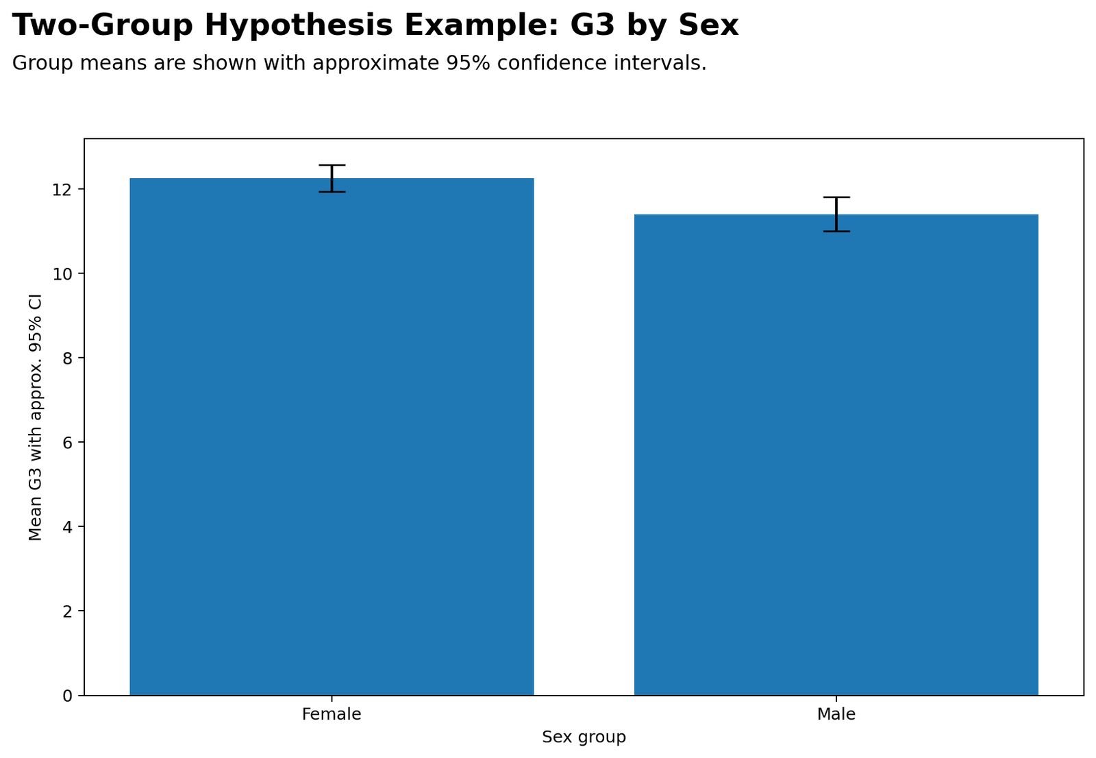
This chart explains the independent-samples hypothesis test. The vertical bars show the mean G3 score for each sex group, and the small error bars show approximate 95% confidence intervals. The female group has a mean of about 12.25, while the male group has a mean of about 11.41. The female bar is visibly higher, meaning the sample difference is about 0.847 grade points. SPSS reports Levene’s test p = .950, so the equal variances assumed row is appropriate. The independent-samples t-test gives t(647) = 3.311, p = .001, with a 95% confidence interval for the difference from 0.345 to 1.350. Since the interval is entirely above zero and the p-value is below .05, the hypothesis decision is to reject H0. The practical interpretation is that female students have a statistically higher mean G3 score than male students in this sample. The chart supports this result visually by showing separation between the group means.
Python Chart 4: Correlation Hypothesis Example for G2 and G3
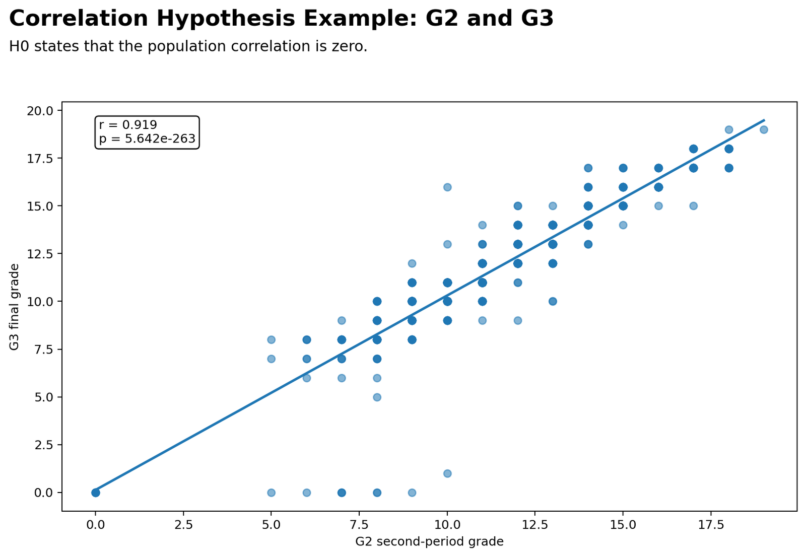
This chart explains the correlation hypothesis test. The x-axis shows G2 second-period grade, and the y-axis shows G3 final grade. Each point represents a student. The fitted line slopes upward, which means higher G2 values are associated with higher G3 values. The chart label reports r = 0.919 and an extremely small p-value. SPSS also reports Pearson r = .919, p < .001, N = 649. The null hypothesis says that the population correlation is zero, meaning no linear relationship. The alternative hypothesis says that the population correlation is not zero. Because the p-value is far below .05, reject H0. The relationship is not only statistically significant; it is also very strong in size. The plot supports this interpretation because the points cluster closely around the upward trend line. Some low-score points are visible, but the overall pattern is strongly positive.
R Chart 1: Null vs Alternative Hypothesis p-value Decisions
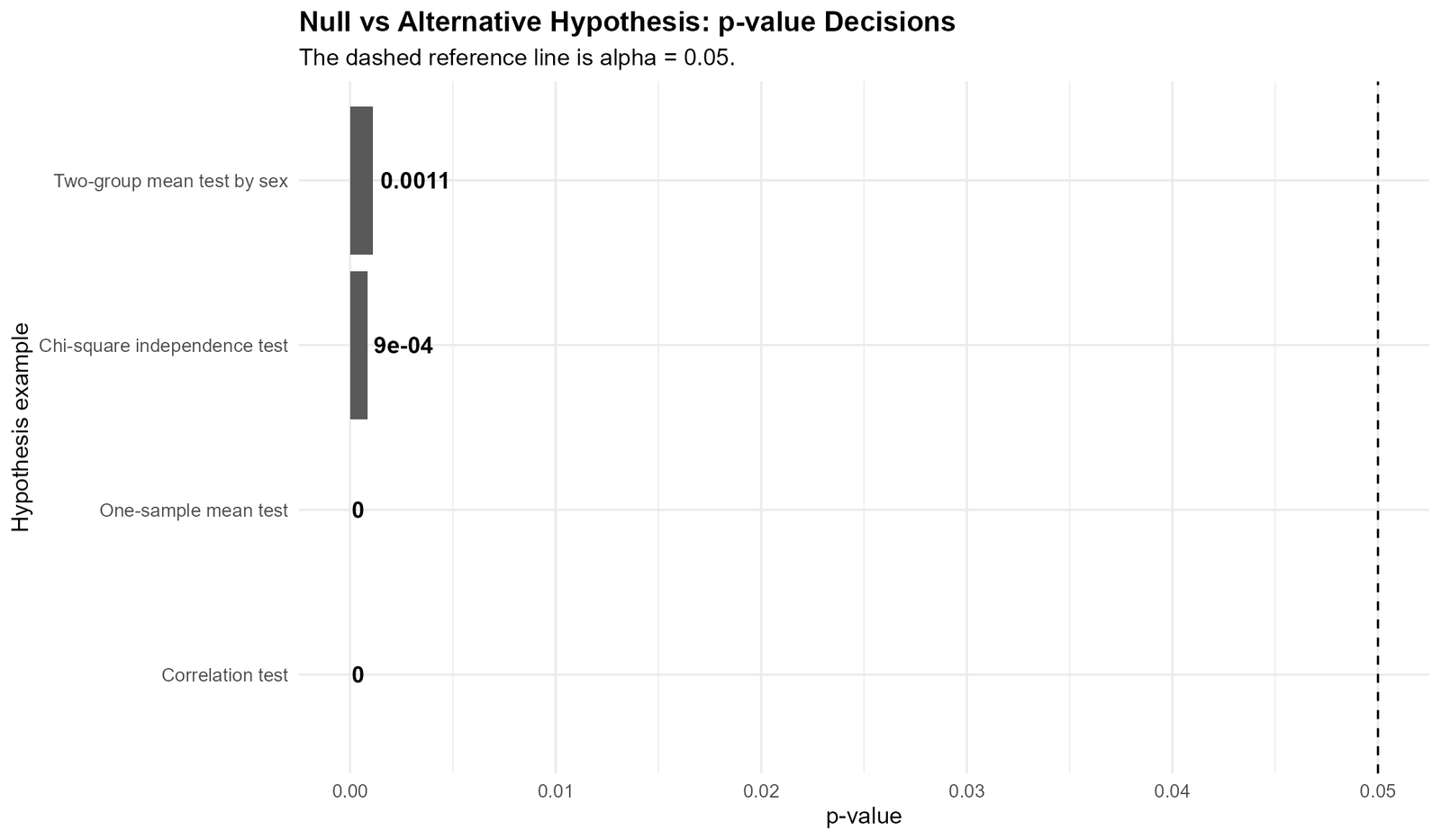
The R p-value decision chart confirms the Python decision chart. The dashed vertical line marks alpha = 0.05. The one-sample mean test and correlation test are displayed as 0 because their p-values are too small for the rounded chart label; in a report, they should be written as p < .001. The chi-square p-value is displayed in scientific notation as about 9e-04, which equals approximately 0.0009. The two-group mean test by sex is about 0.0011. All values are far below .05, so every test falls in the reject-H0 region. This chart is useful for teaching because it places multiple hypothesis tests on the same decision scale and shows that the same p-value logic applies across t-tests, correlation and chi-square tests.
R Chart 2: One-Sample Hypothesis Example for G3
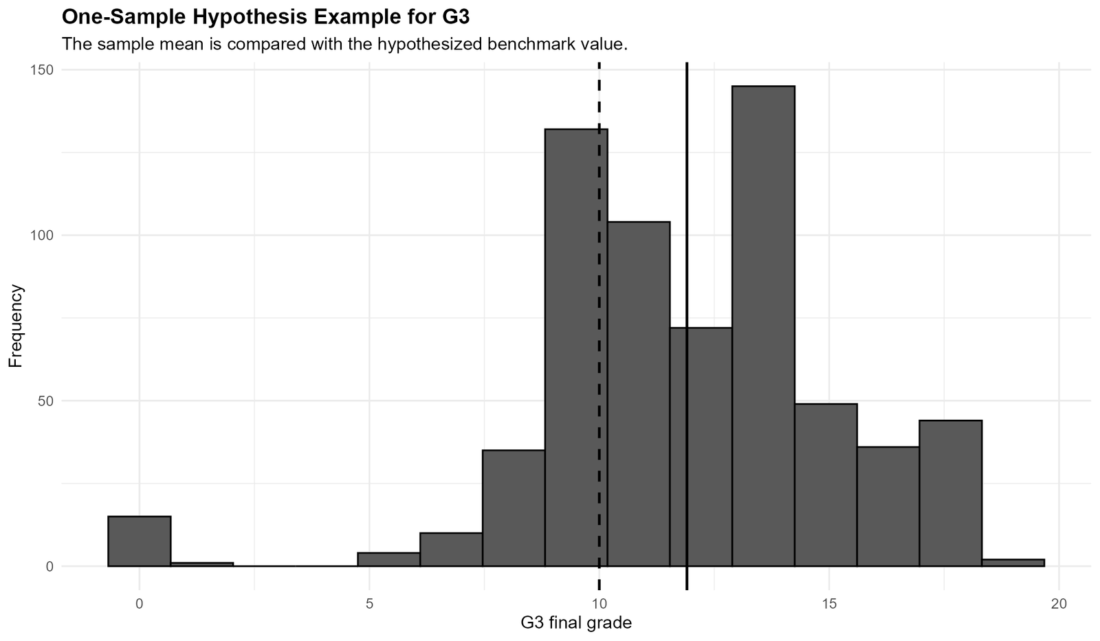
The R one-sample chart repeats the same benchmark comparison. The dashed line marks the null-hypothesis value of 10, while the solid line marks the sample mean near 11.91. The observed distribution has many values above the benchmark, and the sample mean is clearly separated from the hypothesized value. This visual pattern matches the SPSS one-sample t-test result, where t = 15.030 and p < .001. The chart is a direct visual explanation of why the null hypothesis is rejected: the sample mean is not sitting on the benchmark; it is meaningfully higher.
How to Test Null and Alternative Hypotheses in Python, R, SPSS and Excel
Python Workflow
import pandas as pd
from scipy import stats
import scipy.stats as st

df = pd.read_csv("spss_ready_data.csv")

# Example 1: One-sample t-test
# H0: Mean G3 = 10
# H1: Mean G3 != 10
g3 = pd.to_numeric(df["G3"], errors="coerce").dropna()
t_stat, p_value = stats.ttest_1samp(g3, popmean=10)

print("One-sample t-test")
print("H0: Mean G3 = 10")
print("H1: Mean G3 is different from 10")
print("t =", round(t_stat, 3), "p =", p_value)

# Example 2: Two-group t-test by sex
female = df.loc[df["sex"].str.upper().isin(["F", "FEMALE"]), "G3"].astype(float).dropna()
male = df.loc[df["sex"].str.upper().isin(["M", "MALE"]), "G3"].astype(float).dropna()

t2, p2 = stats.ttest_ind(female, male, equal_var=True)
print("Independent-samples t-test")
print("H0: Female and male G3 means are equal")
print("H1: Female and male G3 means are different")
print("t =", round(t2, 3), "p =", p2)

# Example 3: Correlation
g2 = pd.to_numeric(df["G2"], errors="coerce")
g3_all = pd.to_numeric(df["G3"], errors="coerce")
pair = pd.concat([g2, g3_all], axis=1).dropna()
r, p_corr = stats.pearsonr(pair["G2"], pair["G3"])

print("Correlation")
print("H0: Population correlation is zero")
print("H1: Population correlation is not zero")
print("r =", round(r, 3), "p =", p_corr)

# Example 4: Chi-square independence test
table = pd.crosstab(df["school"], df["higher"])
chi2, p_chi, dof, expected = stats.chi2_contingency(table)

print("Chi-square independence test")
print("H0: school and higher are independent")
print("H1: school and higher are associated")
print("chi-square =", round(chi2, 3), "df =", dof, "p =", p_chi)
R Workflow
df <- read.csv("spss_ready_data.csv")

# Example 1: One-sample t-test
# H0: Mean G3 = 10
# H1: Mean G3 is different from 10
one_sample <- t.test(df$G3, mu = 10)
print(one_sample)

# Example 2: Independent-samples t-test by sex
# H0: Mean G3 is equal for female and male students
# H1: Mean G3 differs by sex
two_group <- t.test(G3 ~ sex, data = df, var.equal = TRUE)
print(two_group)

# Example 3: Correlation hypothesis test
# H0: Population correlation is zero
# H1: Population correlation is not zero
corr_test <- cor.test(df$G2, df$G3, method = "pearson")
print(corr_test)

# Example 4: Chi-square independence test
# H0: school and higher are independent
# H1: school and higher are associated
tab <- table(df$school, df$higher)
chi_test <- chisq.test(tab)
print(chi_test)
SPSS Syntax
* Null and Alternative Hypothesis Examples.
* Dataset should already be open as AnalysisData.

TITLE "Null and Alternative Hypothesis - SPSS Output".

DESCRIPTIVES VARIABLES=G1 G2 G3 absences age
 /STATISTICS=MEAN STDDEV MIN MAX.

* Example 1.
* H0: Mean G3 = 10.
* H1: Mean G3 is different from 10.
T-TEST
 /TESTVAL=10
 /MISSING=ANALYSIS
 /VARIABLES=G3
 /CRITERIA=CI(.95).

* Example 2.
* H0: Mean G3 is equal for the two sex groups.
* H1: Mean G3 differs between the two sex groups.
T-TEST GROUPS=sex_num(0 1)
 /MISSING=ANALYSIS
 /VARIABLES=G3
 /CRITERIA=CI(.95).

* Example 3.
* H0: Population correlation is zero.
* H1: Population correlation is not zero.
CORRELATIONS
 /VARIABLES=G2 G3
 /PRINT=TWOTAIL NOSIG
 /MISSING=PAIRWISE.

* Example 4.
* H0: School and higher education intention are independent.
* H1: School and higher education intention are associated.
CROSSTABS
 /TABLES=school BY higher
 /FORMAT=AVALUE TABLES
 /STATISTICS=CHISQ PHI
 /CELLS=COUNT ROW COLUMN EXPECTED
 /COUNT ROUND CELL.

FREQUENCIES VARIABLES=school sex higher
 /ORDER=ANALYSIS.

OUTPUT EXPORT
 /CONTENTS EXPORT=VISIBLE
 /PDF DOCUMENTFILE="D:\DATA ANALYSIS\A Basic Descriptive Statistics Guides\Null and Alternative Hypothesis\SPSS_Output\Null-and-Alternative-Hypothesis-SPSS-Output.pdf".
Excel Workflow
Excel can be used to write hypotheses, calculate test statistics, and apply the p-value decision rule.
| Excel task | Formula or method | Purpose |
|---|---|---|
| One-sample t statistic | =(AVERAGE(G3_range)-10)/(STDEV.S(G3_range)/SQRT(COUNT(G3_range))) | Compares G3 mean with benchmark 10. |
| Two-tailed p-value | =T.DIST.2T(ABS(t_stat), df) | Returns the two-tailed p-value. |
| Correlation | =CORREL(G2_range,G3_range) | Calculates Pearson correlation. |
| Chi-square p-value | =CHISQ.TEST(observed_range, expected_range) | Tests independence in a crosstab. |
| Decision rule | =IF(p_value<0.05,"Reject H0","Fail to reject H0") | Applies alpha = 0.05 decision rule. |
How to Report Null and Alternative Hypothesis Results
One-sample t-test report: A one-sample t-test was conducted to test whether the mean G3 final grade differed from 10. The null hypothesis stated that the population mean was 10, while the alternative hypothesis stated that the population mean differed from 10. The result was significant, t(648) = 15.030, p < .001. The sample mean was 11.91, and the mean difference was 1.906, 95% CI [1.66, 2.16]. Therefore, the null hypothesis was rejected.
Independent-samples t-test report: An independent-samples t-test compared G3 final grades by sex. The null hypothesis stated that female and male students had equal population means. Levene's test was not significant, F = .004, p = .950, so the equal variances assumed row was used. Female students had a higher mean score (M = 12.25, SD = 3.124) than male students (M = 11.41, SD = 3.321). The difference was significant, t(647) = 3.311, p = .001, mean difference = .847, 95% CI [.345, 1.350]. Therefore, the null hypothesis was rejected.
Correlation report: A Pearson correlation tested the relationship between G2 and G3. The null hypothesis stated that the population correlation was zero. The result showed a strong positive correlation, r(647) = .919, p < .001. Therefore, the null hypothesis was rejected. Higher G2 scores were strongly associated with higher G3 final grades.
Chi-square report: A chi-square test of independence tested whether school and higher education intention were independent. The result was significant, χ²(1, N = 649) = 12.024, p = .001. No expected cell count was below 5, and the minimum expected count was 24.03. The association size was small, Cramer's V = .136. Therefore, the null hypothesis of independence was rejected.
When reporting hypothesis tests, always write the null hypothesis, the alternative hypothesis, the test statistic, degrees of freedom when available, p-value, confidence interval when available, and the final decision. If the result is significant, use wording such as reject the null hypothesis. If the result is not significant, use fail to reject the null hypothesis.
Common Mistakes in Null and Alternative Hypothesis Testing
1. Saying “accept the null hypothesis”
In ordinary hypothesis testing, the correct phrase is fail to reject the null hypothesis, not accept the null hypothesis.
2. Writing only the p-value without the hypotheses
A p-value is meaningful only when the reader knows what H0 and H1 were.
3. Treating SPSS .000 as exactly zero
SPSS reports .000 when the p-value is very small. In the written report, use p < .001.
4. Ignoring the direction of the result
After rejecting H0, explain which mean is higher, whether the correlation is positive or negative, or which category pattern creates the association.
5. Ignoring effect size
A significant p-value does not automatically mean the effect is large. The chi-square example is significant, but Cramer's V = .136 indicates a small association. For more, see effect size and coefficient of variation.
6. Using the wrong test for the data type
Use a t-test for mean differences, correlation for numeric relationships, and chi-square for categorical association. For categorical summaries, start with cross tabulation.
7. Forgetting assumptions
Before relying on hypothesis tests, check assumptions. Normality can be checked through Q-Q plots and tests such as Kolmogorov-Smirnov. Variance equality can be checked with Levene test.
Download SPSS Output and Resources
The SPSS output PDF includes descriptive statistics, the one-sample t-test, independent-samples t-test, Pearson correlation, chi-square independence test, crosstabulation, Cramer's V, and frequency tables for school, sex and higher education intention.
External References
FAQs About Null and Alternative Hypothesis
What is a null hypothesis?
A null hypothesis is the default statistical claim. It usually says there is no difference, no relationship, no association, or no effect.
What is an alternative hypothesis?
An alternative hypothesis is the competing research claim. It states that a difference, relationship, association, or effect exists.
What are the symbols for null and alternative hypothesis?
The null hypothesis is usually written as H0. The alternative hypothesis is written as H1 or Ha.
How do you decide whether to reject the null hypothesis?
Compare the p-value with alpha. If p < .05, reject the null hypothesis. If p ≥ .05, fail to reject the null hypothesis.
What does p < .05 mean?
It means the result is statistically significant at the 5% significance level, so the null hypothesis is rejected.
Should I say accept the null hypothesis?
No. In most ordinary hypothesis tests, the correct wording is fail to reject the null hypothesis.
What was the one-sample hypothesis result for G3?
The one-sample t-test compared mean G3 with 10. The result was t(648) = 15.030, p < .001, so the null hypothesis was rejected.
What was the two-group hypothesis result for G3 by sex?
Female students had a higher mean G3 score than male students. The result was t(647) = 3.311, p = .001, so the null hypothesis was rejected.
What was the correlation hypothesis result for G2 and G3?
G2 and G3 had a strong positive correlation, r = .919, p < .001. The null hypothesis of zero correlation was rejected.
What was the chi-square hypothesis result?
The chi-square test showed that school and higher education intention were associated, χ²(1, N = 649) = 12.024, p = .001. The null hypothesis of independence was rejected.

