
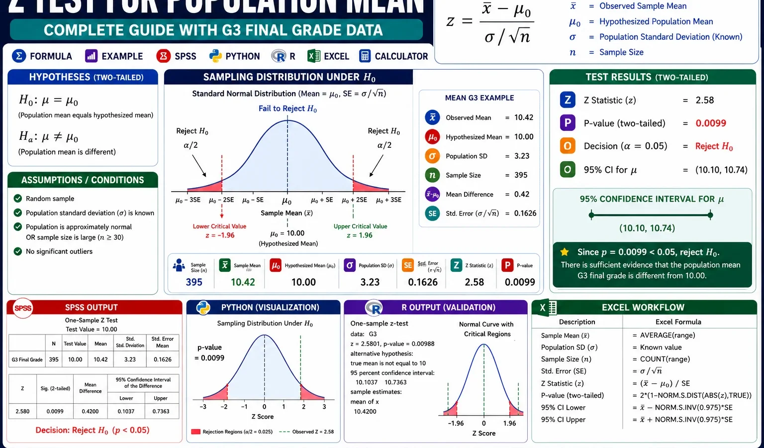
Hypothesis Test for One Population Mean
Z Test for Population Mean is used to test whether an observed sample mean is significantly different from a hypothesized population mean. This guide explains the one sample z test for population mean with formula, assumptions, p-value, confidence interval, SPSS image output, Python charts, R validation charts and Excel workflow using G3 final grade data.
Quick Answer: Z Test for Population Mean Result
The Z Test for Population Mean was performed to test whether the observed mean G3 final grade was significantly different from the hypothesized population mean of 10.000. The image output shows an observed sample mean of 11.906. Therefore, the observed-minus-hypothesized mean difference is 1.906.
The sampling-distribution image under H0 gives acceptance limits of [9.769, 10.231]. The observed mean of 11.906 is far above the upper acceptance limit. The standard normal curve image reports observed z = 16.19 with critical values ±1.96. The confidence interval image reports a 95% confidence interval of [11.675, 12.137]. Because this interval is entirely above 10.000, the null hypothesis is rejected.
Final conclusion: The observed G3 mean is significantly higher than the hypothesized mean of 10.000. The z statistic is far beyond the usual rejection boundary, and the 95% confidence interval does not include the null mean. Therefore, the data provide strong evidence that the population mean G3 score is greater than the hypothesized benchmark.
Important reporting note: If software displays a very small p-value as .000, do not write p = .000. Write p < .001. The charted z value of 16.19 is extremely far from zero, so the p-value is far below .001.
Table of Contents
- What Is a Z Test for Population Mean?
- When Should You Use It?
- Null and Alternative Hypothesis
- Z Test for Population Mean Formula
- Conditions and Assumptions
- Dataset and Variable Used
- Verified Results Summary
- SPSS Image Output and Interpretation
- Python Charts and Interpretation
- R Validation Charts and Interpretation
- Overall Image Interpretation
- How to Run the Test in SPSS, Python, R and Excel
- How to Report the Z Test for Population Mean
- Common Mistakes
- Related Statistical Guides
- FAQs
What Is a Z Test for Population Mean?
A Z Test for Population Mean is a hypothesis test used to compare one observed sample mean with one hypothesized population mean. It is also called a one sample z test for population mean, z test for one population mean, one population z test for the mean or one-sample z test for the population mean.
The test answers a question such as: Is the average G3 final grade different from 10? The observed mean is compared with the hypothesized mean. The difference is then standardized into a z statistic. That z statistic is interpreted using the standard normal distribution.
In this worked example, the hypothesized population mean is 10.000, and the observed sample mean is 11.906. The observed mean is higher than the hypothesized mean by 1.906 grade points. The charted z statistic is 16.19, which is far outside the usual acceptance region.
For background concepts, see Null and Alternative Hypothesis, P Value, Z Score, Standard Error, Standard Normal Distribution, Mean, Median and Mode and Descriptive Statistics.
When Should You Use a Z Test for Population Mean?
Use a z test for population mean when the goal is to test one observed sample mean against one hypothesized population mean. The outcome should be numeric, and the test should be based on a known population standard deviation or a valid large-sample z workflow.
| Situation | Use Z Test for Population Mean? | Reason |
|---|---|---|
| Testing whether mean G3 differs from 10 | Yes | G3 is numeric, and the comparison is against one hypothesized mean. |
| Testing whether average exam score is higher than a fixed benchmark | Yes | The outcome is continuous and the benchmark is one population mean value. |
| Testing whether one sample mean differs from a known historical mean | Yes | The test compares one observed mean with one reference mean. |
| Comparing two school means, such as GP vs MS | No | That is a two-group mean question. Use a Two Sample Z Test or a two-sample t test. |
| Testing whether a pass proportion differs from 50% | No | That is a proportion question. Use a One Proportion Z Test. |
The keyword phrase when to use z test for population mean is important because many students confuse this test with the t test. A textbook z test assumes the population standard deviation is known. If the population standard deviation is unknown and estimated from the sample, a one-sample t test is usually the formal textbook option.
Null and Alternative Hypothesis for Z Test for Population Mean
The hypotheses compare the population mean with the hypothesized value. In this example, the hypothesized mean is 10.000.
| Hypothesis | Symbolic form | Meaning in this example |
|---|---|---|
| Null hypothesis | H0: μ = 10.000 | The population mean G3 final grade equals 10. |
| Alternative hypothesis | H1: μ ≠ 10.000 | The population mean G3 final grade is different from 10. |
| Observed result | x̄ = 11.906 | The observed sample mean is higher than the hypothesized mean. |
| Decision rule | Reject H0 if |z| > 1.96 or p < .05 | The observed z = 16.19 is far beyond the rejection boundary. |
This post uses a two-tailed z test because the alternative hypothesis is written as “different from 10.” If the research question were specifically whether the mean is higher than 10, the alternative would be H1: μ > 10. The observed mean is higher than 10, so the direction of the result is positive.
Z Test for Population Mean Formula and Calculation
The z test for population mean formula is:
z = (x̄ - μ0) / SE

where:
x̄  = observed sample mean
μ0  = hypothesized population mean
SE  = standard error of the sample mean
Using the exact values displayed in the image output:
| Component | Exact image value | Interpretation |
|---|---|---|
| Hypothesized mean | 10.000 | The null benchmark for the population mean. |
| Observed sample mean | 11.906 | The sample mean G3 final grade. |
| Observed − hypothesized | 1.906 | The sample mean is 1.906 grade points above the null mean. |
| Acceptance limits under H0 | [9.769, 10.231] | Expected range of sample means under the null hypothesis at α = .05. |
| Z statistic | 16.19 | The observed mean is extremely far from the null mean in standard-error units. |
| Critical z values | ±1.96 | Two-tailed rejection boundaries at α = .05. |
| 95% confidence interval | [11.675, 12.137] | The estimated population mean range is entirely above 10. |
Observed mean = 11.906
Hypothesized mean = 10.000

Observed - hypothesized = 11.906 - 10.000
Observed - hypothesized = 1.906

Observed z = 16.19
Critical z = ±1.96

Decision: reject H0
The confidence interval confirms the same decision:
95% CI for population mean = [11.675, 12.137]

Because 10.000 is not inside this interval,
the hypothesized mean is not supported by the sample.
For more detail on intervals and standard errors, see Confidence Interval, Margin of Error and Standard Error.
Conditions and Assumptions for Z Test for Population Mean
The assumptions for z test population mean explain when the test result can be trusted. The main assumptions are about the outcome scale, independence, standard error and normal approximation.
| Condition | How to check it | This example |
|---|---|---|
| Numeric outcome | The dependent variable should be measured numerically. | G3 final grade is a numeric score. |
| One sample mean | The test should compare one observed mean with one hypothesized mean. | The observed G3 mean is compared with μ0 = 10.000. |
| Independent observations | Each row should represent a separate case. | Student records are treated as independent observations. |
| Known standard deviation or valid z workflow | A textbook z test assumes known population standard deviation. | The image output reports the z-test result directly through the sampling distribution and z curve. |
| Approximately normal sampling distribution | The sampling distribution of the mean should be approximately normal. | The sampling-distribution image under H0 is approximately normal. |
If the population standard deviation is unknown and only the sample standard deviation is available, a one-sample t test is normally used. This is the key difference between z and t test for population mean: the z test uses a known standard deviation or z-standardized workflow, while the t test estimates uncertainty using the sample standard deviation and t distribution.
Dataset and Variable Used
This worked example uses student performance data. The outcome variable is G3 final grade. The z test for population mean compares the observed average G3 score with the hypothesized mean of 10.000.
| Item | Value from images | Explanation |
|---|---|---|
| Outcome variable | G3 | Final grade score. |
| Hypothesized mean | 10.000 | Population mean claimed under the null hypothesis. |
| Observed mean | 11.906 | Observed sample mean G3 score. |
| Observed difference | 1.906 | Observed mean minus hypothesized mean. |
| Subgroup context | GP = 12.577, MS = 10.650 | Mean G3 by school, used only as descriptive context. |
External dataset source: UCI Machine Learning Repository: Student Performance dataset.
Verified SPSS, Python and R Results Summary
The SPSS image output, Python charts and R validation charts all support the same conclusion. The observed G3 mean is above the hypothesized population mean. The observed mean is 11.906, while the hypothesized mean is 10.000. The difference is 1.906. The z statistic is 16.19, and the confidence interval is entirely above the hypothesized mean.
| Statistic | Exact image value | Interpretation |
|---|---|---|
| Hypothesized mean | 10.000 | The benchmark under H0. |
| Observed sample mean | 11.906 | The sample mean is higher than the benchmark. |
| Observed minus hypothesized | 1.906 | The observed mean is 1.906 points above H0. |
| Acceptance limits under H0 | [9.769, 10.231] | The observed mean is far outside the acceptance range. |
| Z statistic | 16.19 | The observed mean is far into the rejection region. |
| Critical values | ±1.96 | Two-tailed α = .05 boundaries. |
| 95% confidence interval | [11.675, 12.137] | The interval is entirely above 10.000. |
| Decision | Reject H0 | The population mean is significantly different from 10.000. |
SPSS Image Output and Interpretation
The SPSS image output explains the z test for population mean visually. These images show the G3 distribution, the hypothesized mean, the observed mean, the observed-minus-hypothesized difference, the sampling distribution under H0, the standard normal z curve, the confidence interval and the descriptive school mean context.
1. SPSS Image: G3 Distribution with Hypothesized and Observed Mean
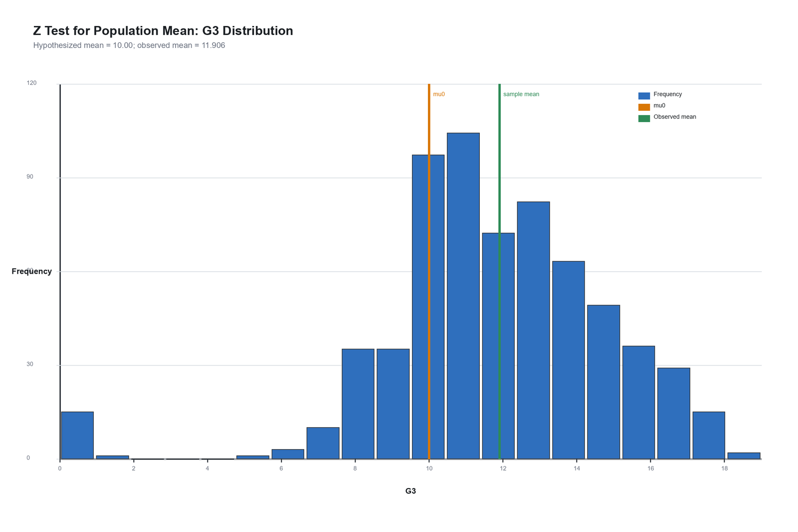
This SPSS image shows the distribution of G3 final grades. The orange line marks the hypothesized mean of 10.000, while the green line marks the observed sample mean of 11.906. The observed mean line is clearly to the right of the hypothesized mean line.
The chart is important because it shows the test comparison in the original grade scale. Before using a formula, the reader can see that the sample average is higher than the null benchmark. The difference is 1.906 grade points.
This distribution image supports the final decision because the observed mean is not close to the null value. The later sampling distribution and z curve show that the distance is statistically extreme.
2. SPSS Image: Hypothesized Mean versus Observed Sample Mean
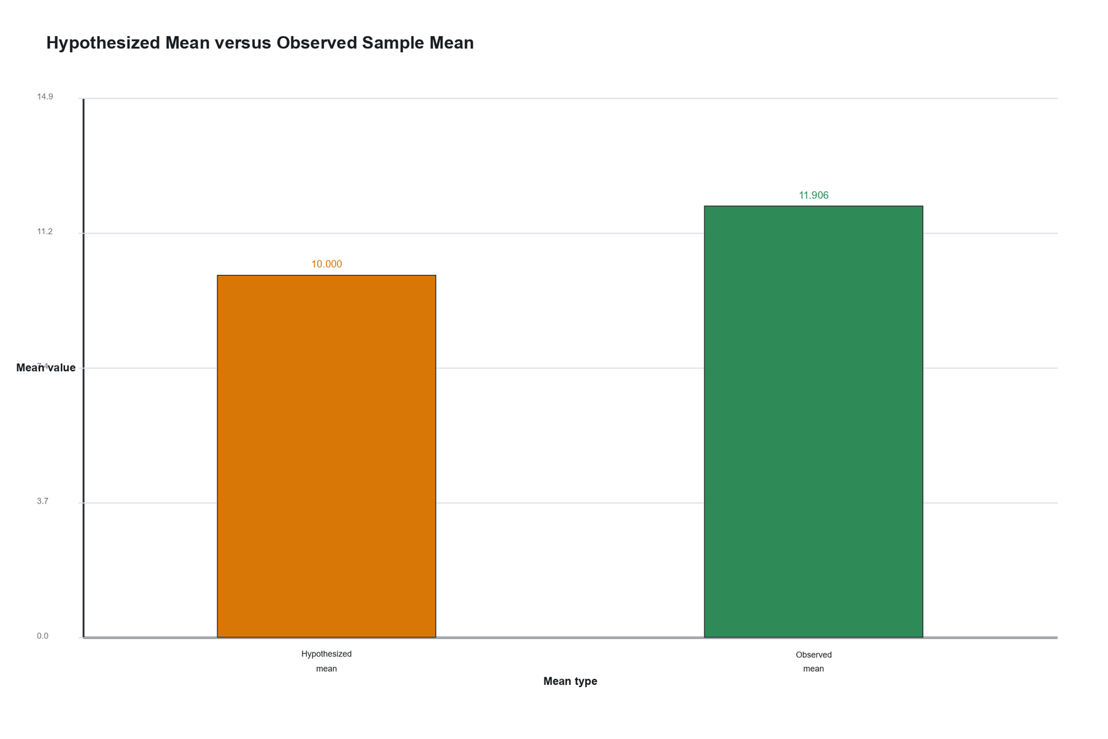
This SPSS image focuses directly on the two mean values. The hypothesized mean is 10.000, and the observed sample mean is 11.906. The observed mean is higher.
This chart is the simplest visual explanation of the hypothesis test. The null hypothesis says the population mean equals 10. The sample gives an observed mean of 11.906. The z test asks whether this difference is too large to be explained by random sampling variation.
The chart supports the conclusion because the observed mean is visibly above the null mean. The formal z statistic of 16.19 confirms that the gap is statistically significant.
3. SPSS Image: Observed Minus Hypothesized Mean
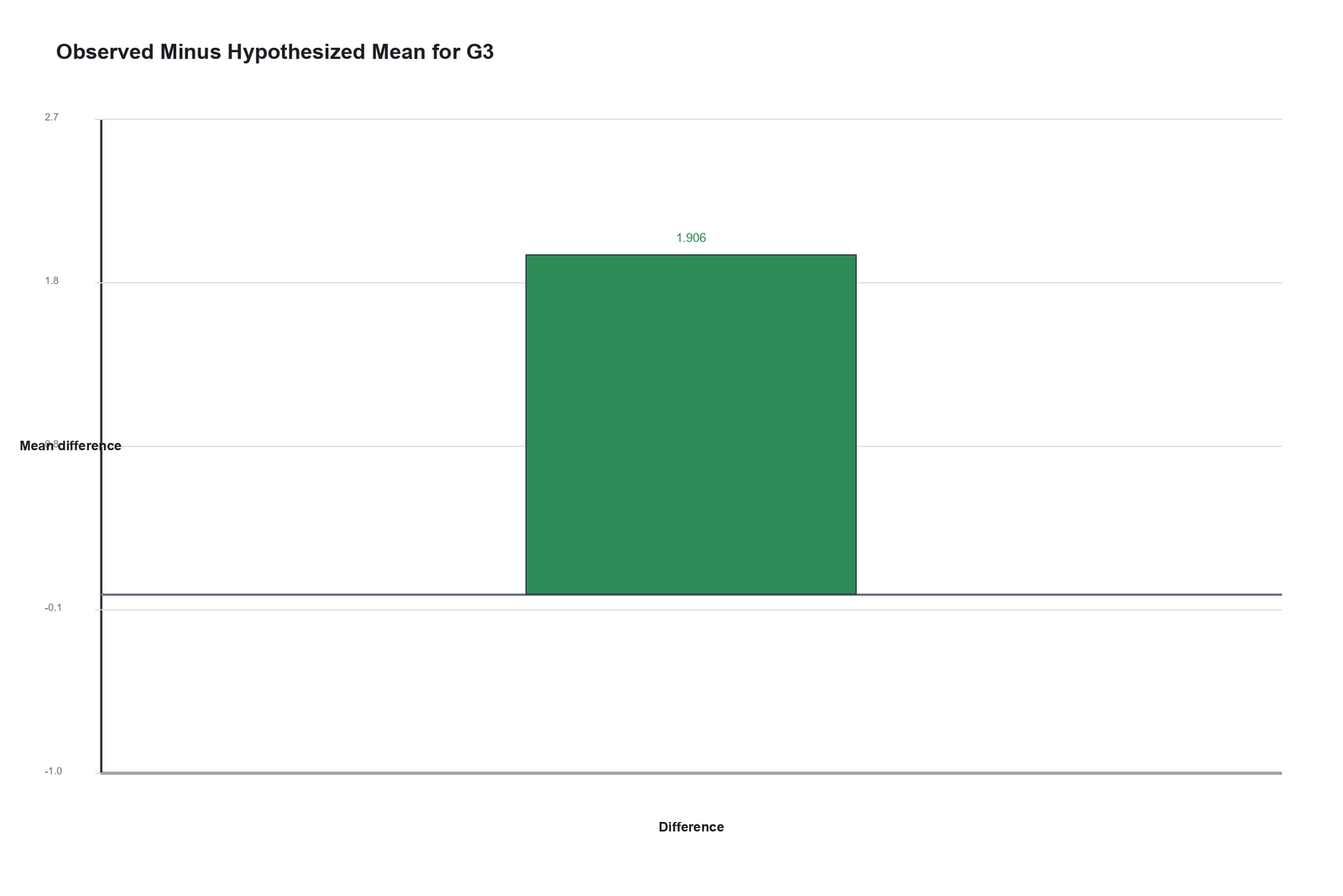
This SPSS image isolates the difference between the observed mean and the hypothesized mean. The displayed difference is 1.906. This value is the numerator of the z test formula.
The chart is useful because it changes the comparison from two separate bars into one direct effect size. Instead of only saying that 11.906 is higher than 10.000, it reports the exact distance: 1.906 grade points.
Since the difference is positive, the observed mean is above the hypothesized mean. The z test then standardizes this positive difference by the standard error to determine statistical significance.
4. SPSS Image: Sampling Distribution of Sample Mean Under H0
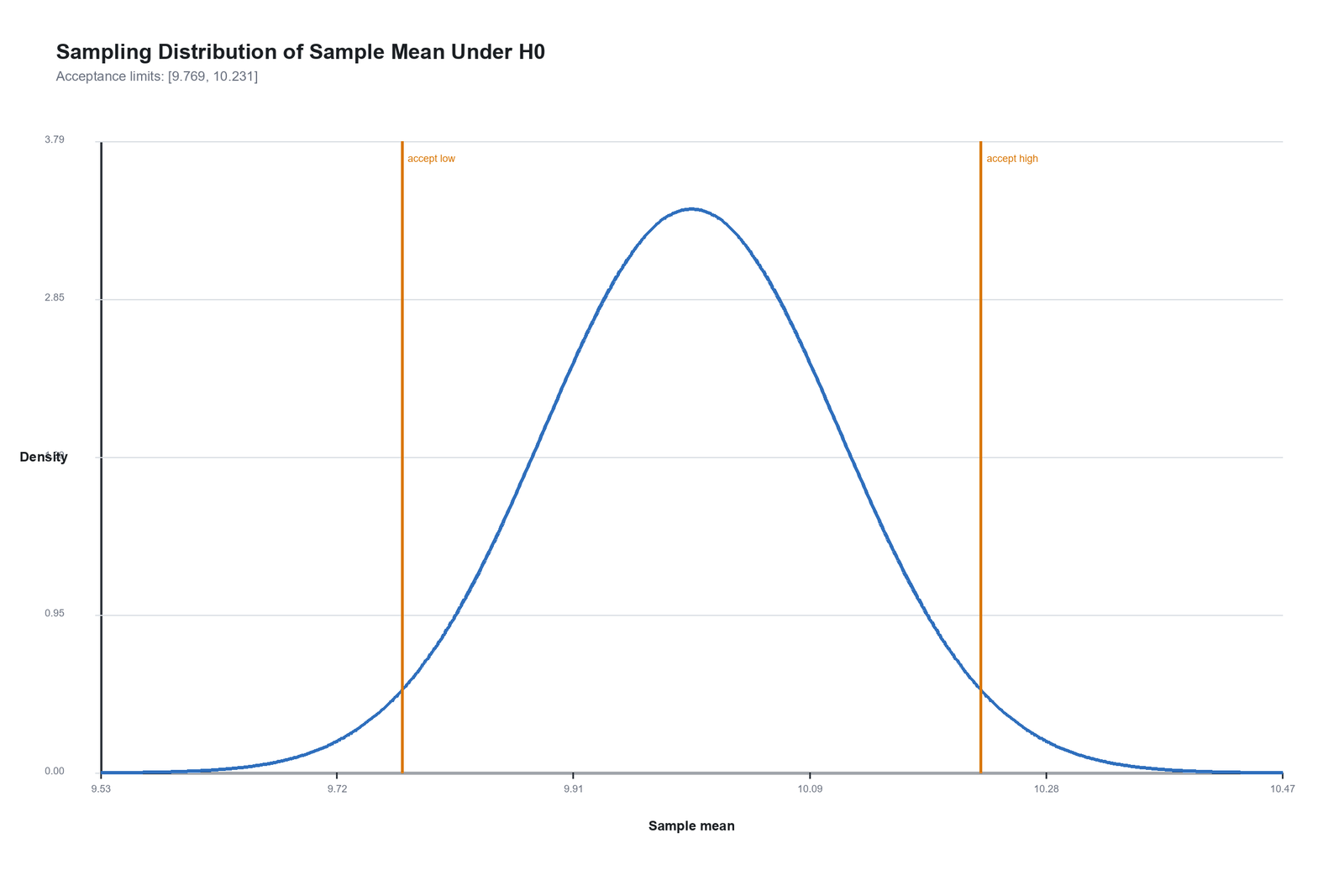
This SPSS image shows the expected sampling distribution of the sample mean if the null hypothesis were true. Under H0, the center of the sampling distribution is the hypothesized mean of 10.000. The image displays acceptance limits of [9.769, 10.231].
The acceptance limits show the range of sample means that would be considered ordinary under the null hypothesis at the displayed decision level. The observed mean, 11.906, is far above the upper acceptance limit of 10.231.
This image is one of the strongest visual explanations of the result. It shows that the observed mean is not merely a little above 10; it lies far outside the range expected under H0. Therefore, the null hypothesis should be rejected.
5. SPSS Image: Z Statistic on the Standard Normal Curve
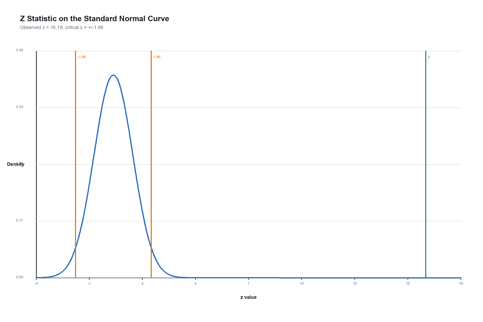
This SPSS image places the observed z statistic on the standard normal curve. The observed value is z = 16.19. The chart also shows the usual two-tailed critical values, -1.96 and +1.96.
The observed z value is far to the right of +1.96. This means the observed mean is extremely far from the null mean after standardization. Under the null hypothesis, a z value this extreme would be extraordinarily unlikely.
The correct decision is to reject the null hypothesis. In report language, the result is statistically significant, and the p-value should be written as p < .001.
6. SPSS Image: Confidence Interval for Population Mean
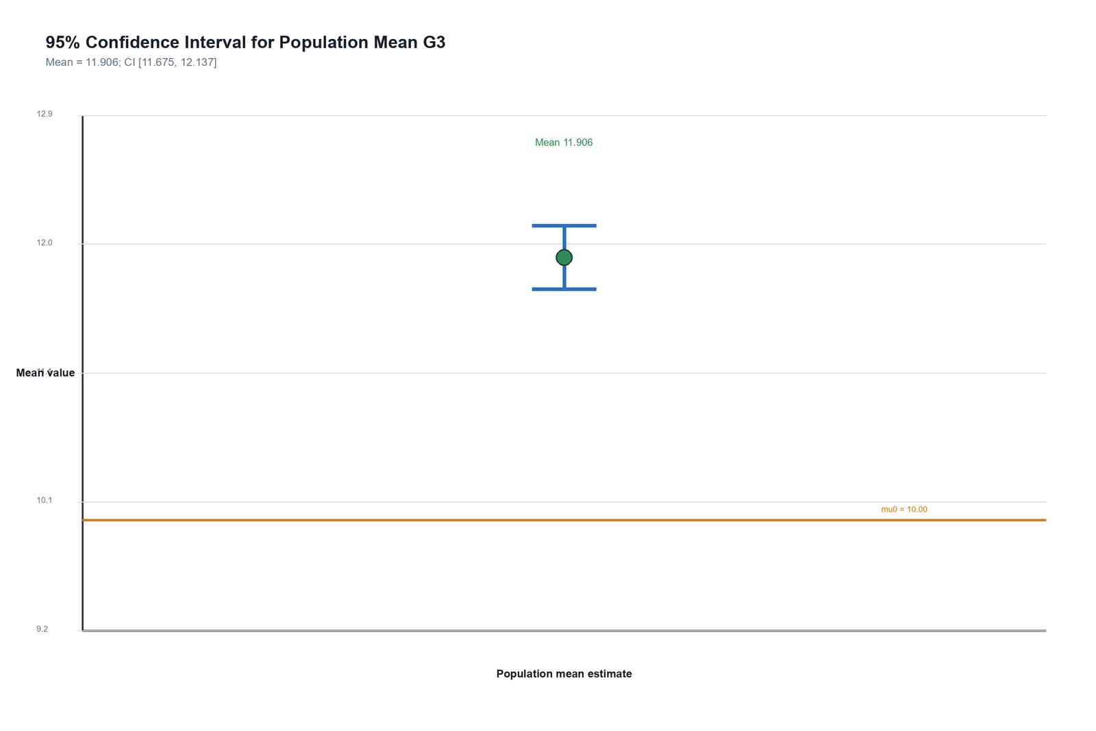
This SPSS image shows the estimated 95% confidence interval for the population mean G3 score. The observed mean is 11.906, and the confidence interval is [11.675, 12.137].
The hypothesized mean of 10.000 is not inside this interval. In fact, the full interval is well above 10. This supports the same conclusion as the z statistic: the observed data are not consistent with a population mean of 10.
The confidence interval also gives practical meaning. It suggests that the population mean G3 score is likely around the high 11s to low 12s, not around 10.
7. SPSS Image: Mean G3 by School
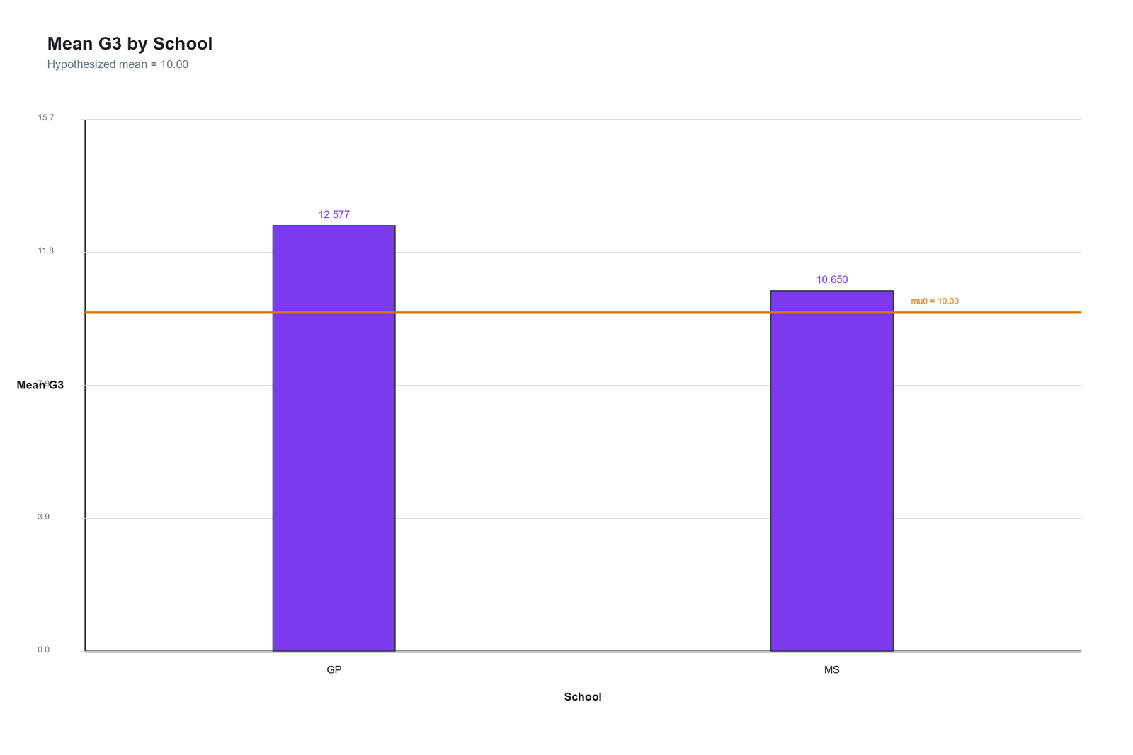
This SPSS image provides descriptive school context. The GP school has a mean G3 score of 12.577, and the MS school has a mean G3 score of 10.650. Both means are above the hypothesized mean line of 10.000, but GP is clearly higher than MS.
This image does not change the main z test for population mean because the formal test compares the overall observed mean of 11.906 with the hypothesized population mean of 10.000. The school chart is included as descriptive context.
If the research question is whether GP and MS differ significantly from each other, a separate two-sample test should be used. In this article, the school chart helps explain the structure behind the overall G3 mean.
Python Charts and Interpretation
The Python charts validate the same z test for population mean using a programmatic workflow. They repeat the distribution, mean comparison, observed-minus-hypothesized difference, sampling distribution, z curve, confidence interval and school mean context.
1. Python Chart: Distribution with Hypothesized and Observed Mean
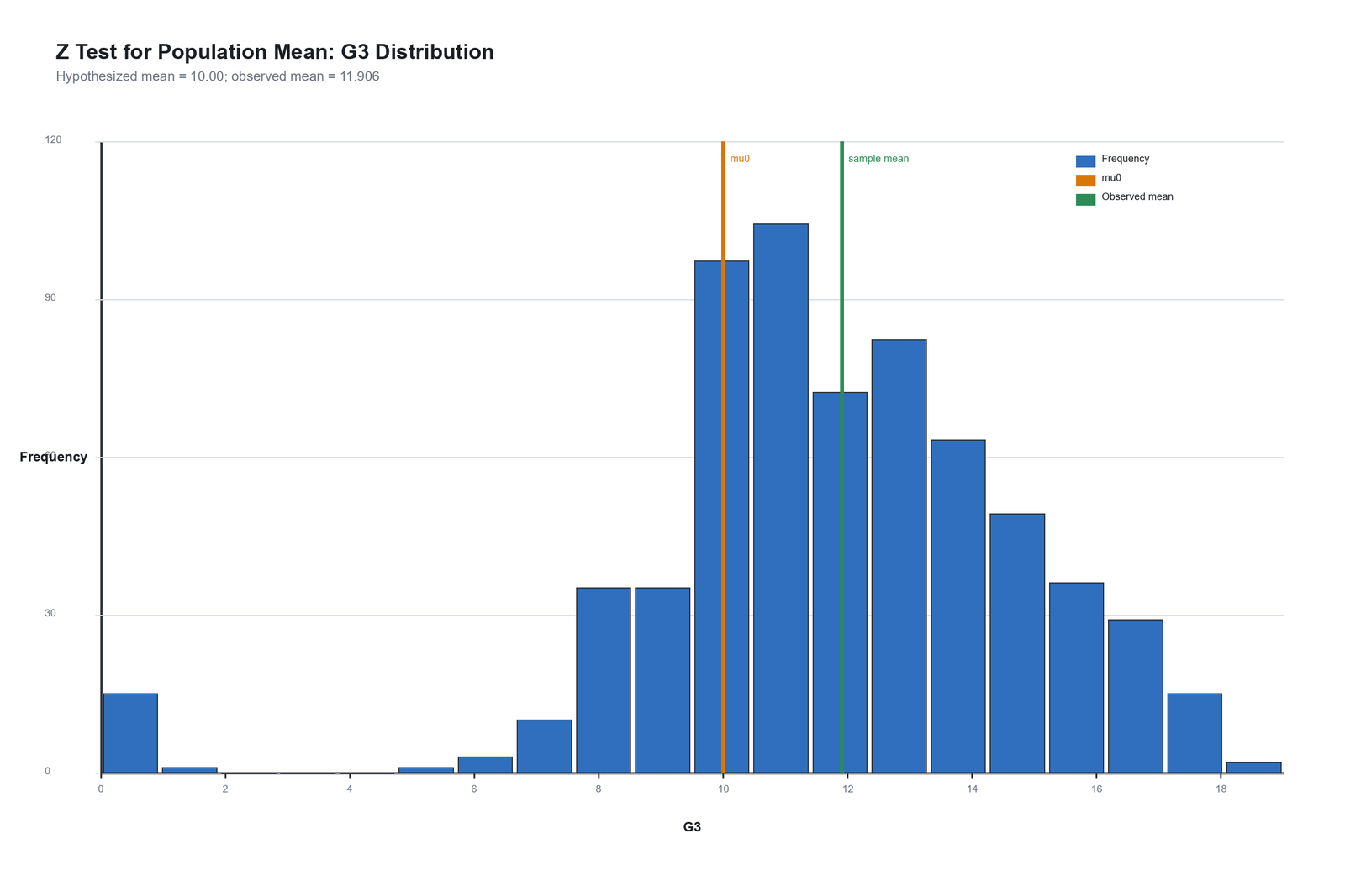
The Python distribution chart confirms the same pattern shown in the SPSS output. The hypothesized mean line is at 10.000, while the observed mean line is at 11.906. The observed mean is to the right of the null benchmark.
This chart shows the raw grade distribution and the location of the two important mean values. The visual separation between the two lines is the practical difference being tested.
The Python chart supports the same conclusion as SPSS: the observed mean is higher than the hypothesized population mean, and the later z curve confirms that the difference is statistically significant.
2. Python Chart: Hypothesized Mean versus Observed Mean
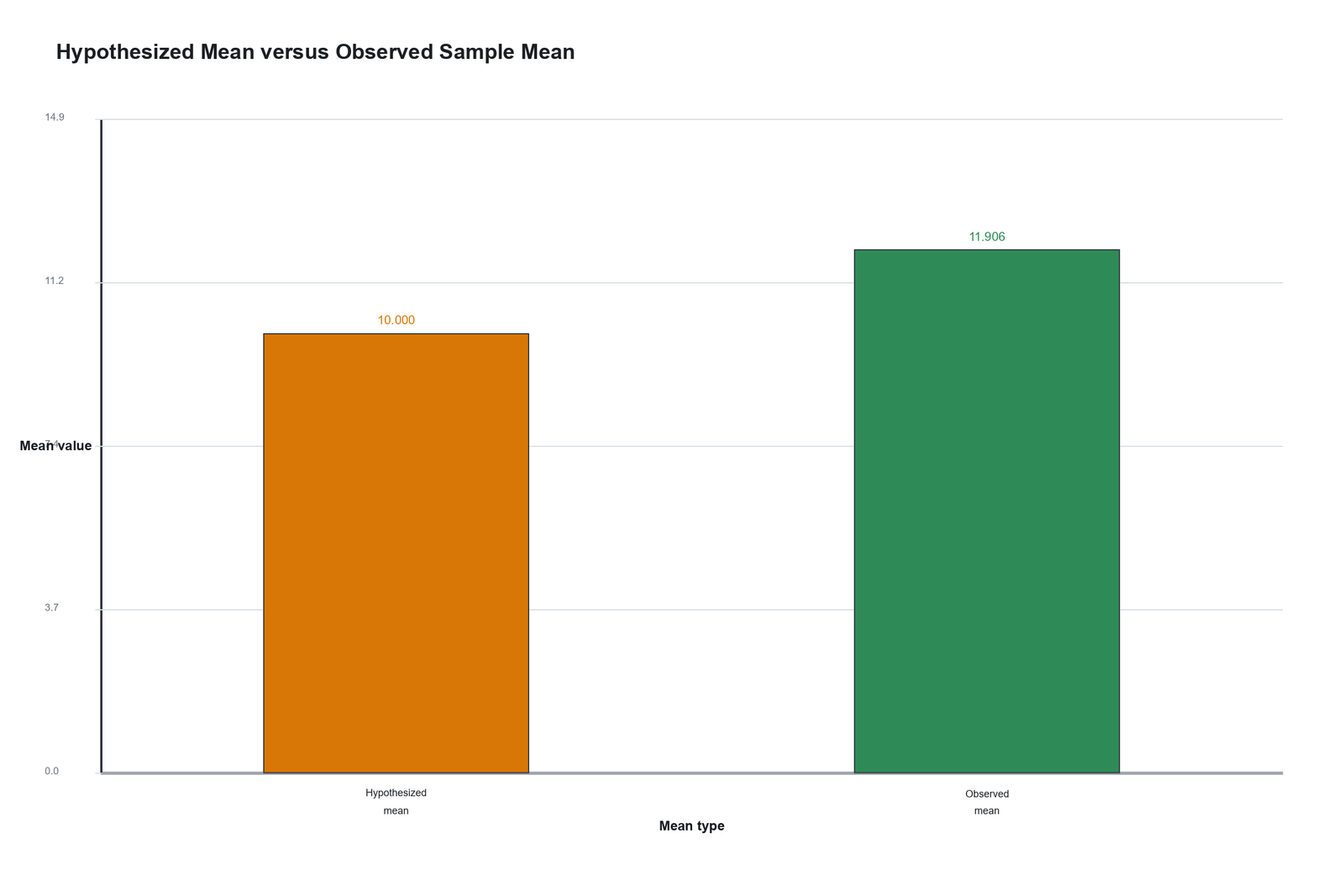
The Python mean-comparison chart shows two values: the hypothesized mean of 10.000 and the observed sample mean of 11.906. The observed mean is higher by 1.906.
This is the central comparison in the z test for population mean. The chart tells the reader exactly what is being tested: whether a sample mean of 11.906 is too far from a hypothesized population mean of 10.
Because the difference is large and positive, the resulting z statistic is also large and positive.
3. Python Chart: Observed Minus Hypothesized Mean
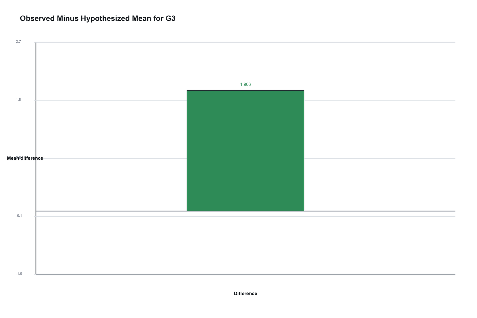
The Python difference chart reports the exact observed-minus-hypothesized value: 1.906. This means the sample mean is 1.906 G3 grade points above the hypothesized value.
This chart is helpful because it turns the comparison into one clear number. It also makes it easy to explain the direction of the result: the difference is positive, so the observed mean is higher than the hypothesized mean.
The z statistic standardizes this positive difference by the standard error. Since the charted z statistic is 16.19, the standardized difference is very large.
4. Python Chart: Sampling Distribution Under H0
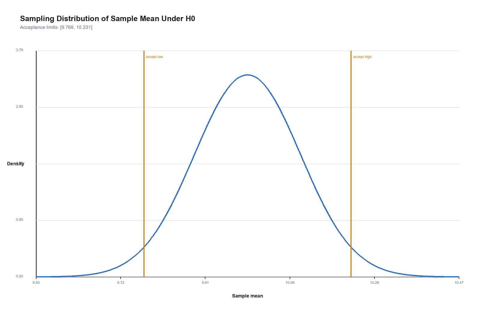
The Python sampling distribution chart shows what sample means would look like if the null hypothesis were true. The center is the hypothesized mean of 10.000, and the acceptance limits are [9.769, 10.231].
The observed mean is 11.906, which is far above the upper acceptance limit of 10.231. This means the observed mean is not compatible with ordinary variation under H0.
This chart gives a very strong visual explanation of the decision. The observed mean is outside the expected H0 range, so the null hypothesis should be rejected.
5. Python Chart: Z Statistic on the Standard Normal Curve
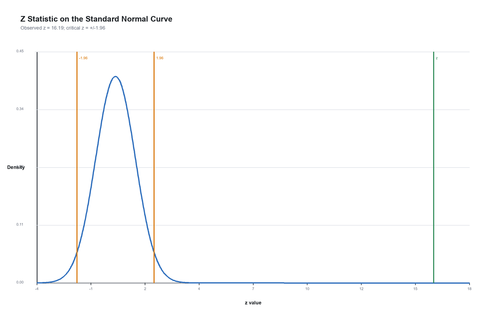
The Python standard normal curve shows the observed z statistic of 16.19. The critical values are -1.96 and +1.96. The observed z is far to the right of the positive critical value.
This confirms the formal test decision. If the null hypothesis were true, the z statistic would usually fall near zero and rarely beyond ±1.96. A value of 16.19 is far outside the expected range.
The Python chart supports reporting the result as statistically significant, with p < .001.
6. Python Chart: Confidence Interval for Population Mean
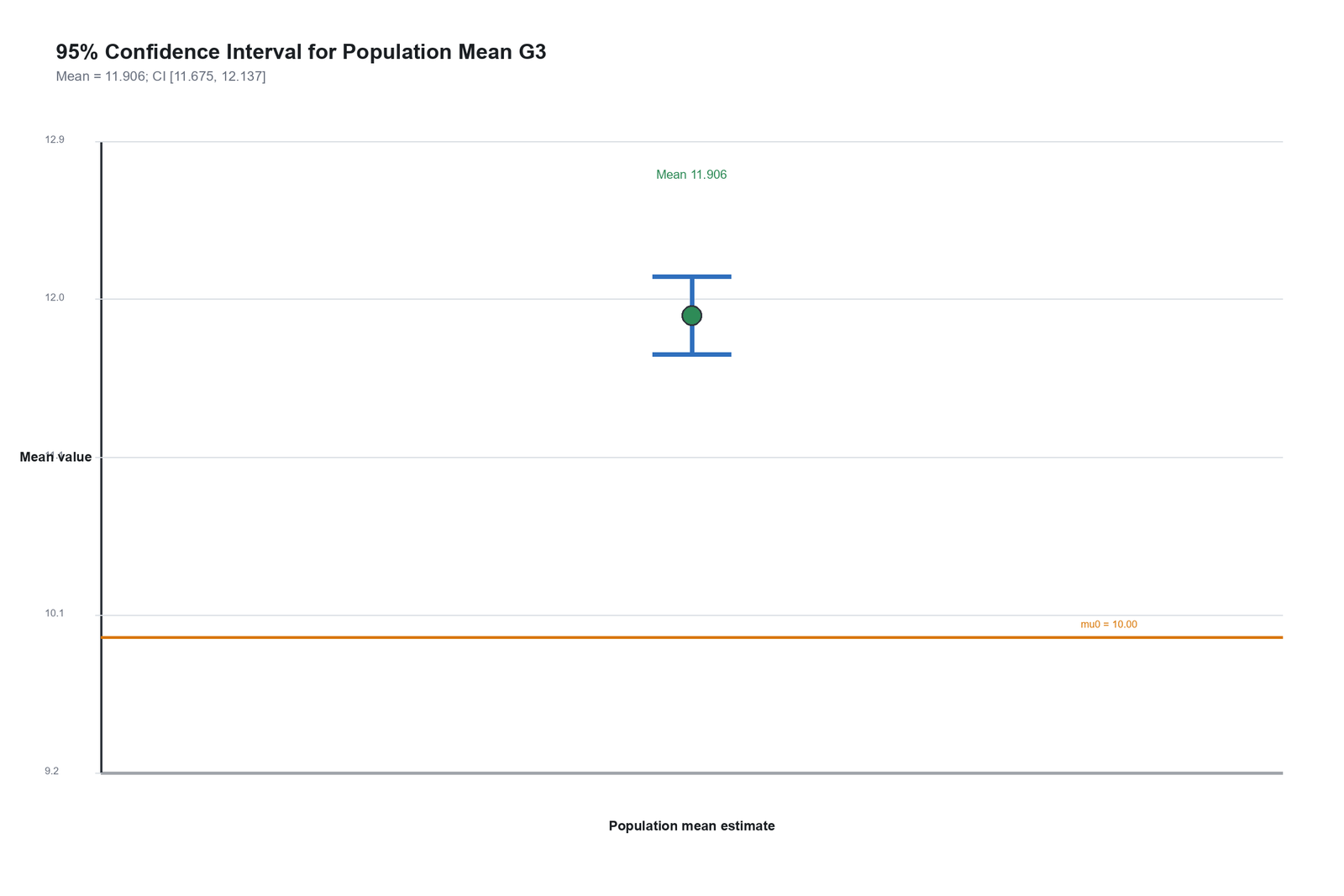
The Python confidence interval chart gives the same interval estimate as SPSS: [11.675, 12.137]. The point estimate is 11.906.
The null mean of 10.000 is far below the interval. This means the estimated population mean is not close to the hypothesized value.
The confidence interval supports both statistical and practical interpretation: the estimated population mean G3 is likely around 11.7 to 12.1, not 10.
7. Python Chart: Mean G3 by School
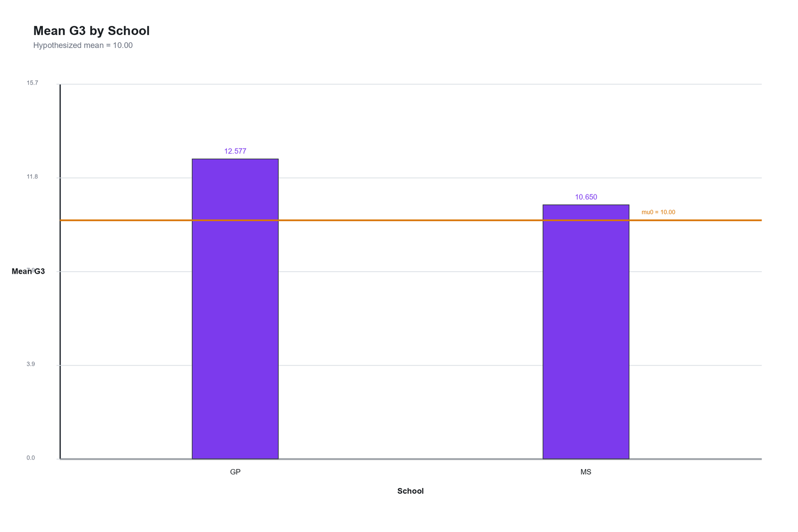
The Python school chart gives subgroup context. It shows that GP has a mean G3 of 12.577, while MS has a mean G3 of 10.650. Both are above the hypothesized mean line of 10, but GP is higher.
This image helps readers understand the overall observed mean of 11.906. The overall mean reflects the distribution of students across schools and the different school-level averages.
The chart is descriptive only. It does not replace a formal two-group test. The main z test in this article remains the comparison between the overall observed mean and the hypothesized population mean.
R Validation Charts and Interpretation
The R validation charts provide another software check for the same result. R repeats the distribution view, mean comparison, observed-minus-hypothesized difference, sampling distribution, z curve, confidence interval and school context.
1. R Chart: Distribution with Hypothesized and Observed Mean
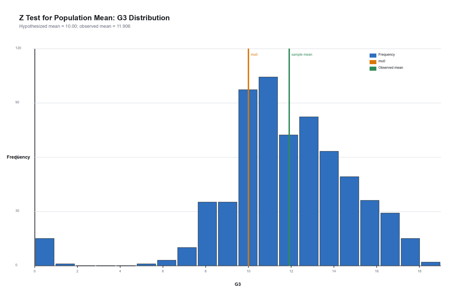
The R distribution chart confirms the same result shown by SPSS and Python. The hypothesized mean is 10.000, and the observed mean is 11.906. The observed mean is shifted to the right of the hypothesized value.
This chart validates the raw comparison behind the test. The sample center is higher than the null benchmark by 1.906 grade points.
Because R confirms the same distribution-level story, it supports the consistency of the analysis across software outputs.
2. R Chart: Hypothesized Mean versus Observed Mean
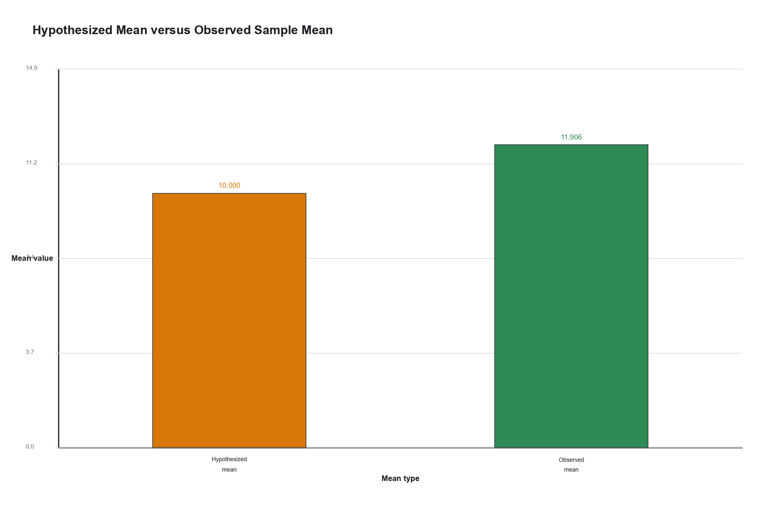
The R mean-comparison chart confirms that the observed mean is above the hypothesized mean. The values are 11.906 versus 10.000.
This chart directly represents the core hypothesis-test comparison. The null hypothesis says the population mean equals 10. The observed sample mean is 11.906.
The R chart validates the same conclusion as the SPSS and Python images: the observed mean is clearly higher than the null value.
3. R Chart: Observed Minus Hypothesized Mean
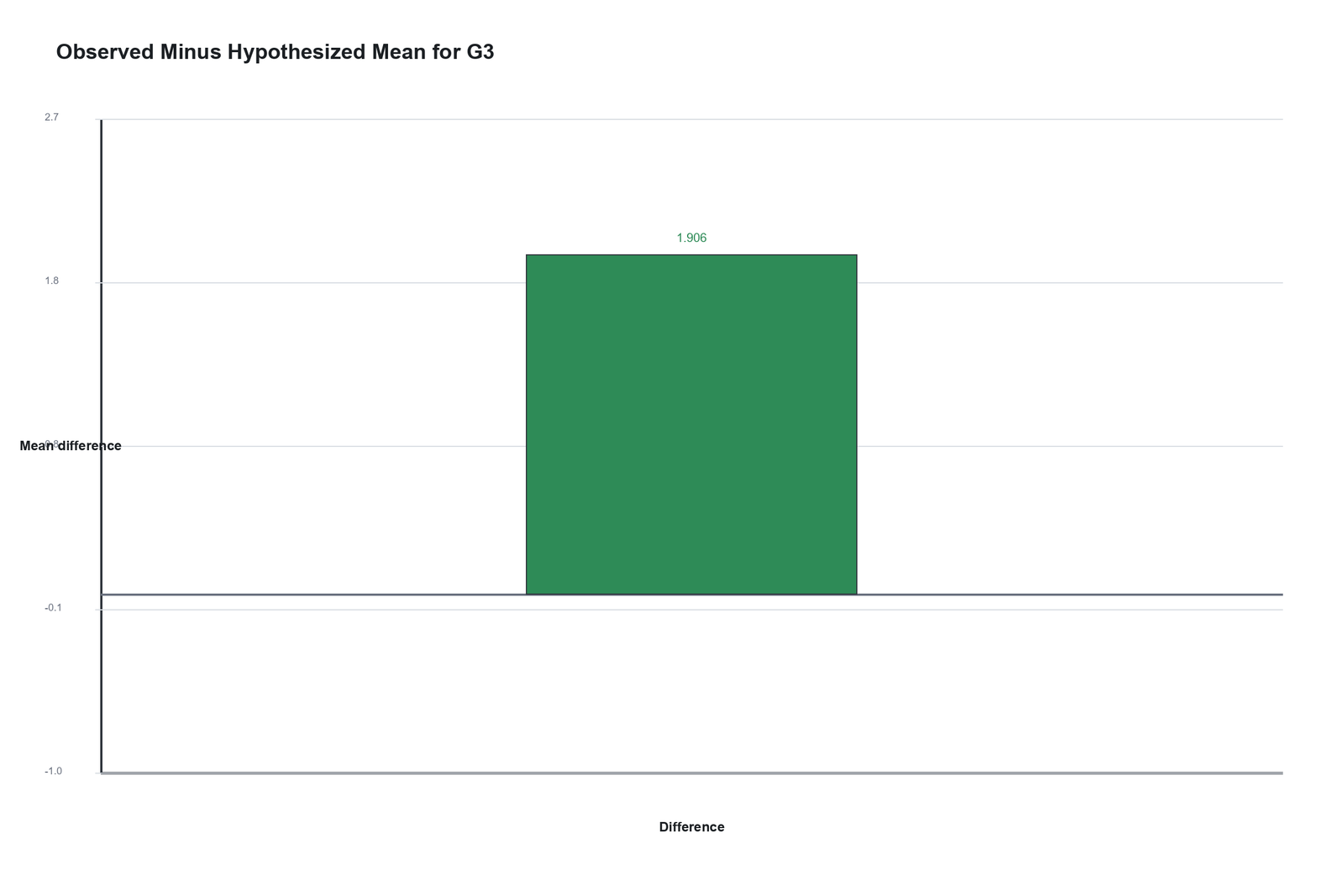
The R difference chart confirms the exact mean difference of 1.906. This is the observed mean minus the hypothesized mean.
The positive value means the observed G3 mean is higher than 10.000. This direction matters because it tells the reader that the result is not only statistically significant but also above the benchmark.
The chart supports the formula-based interpretation because the z statistic begins with this difference in the numerator.
4. R Chart: Sampling Distribution Under H0
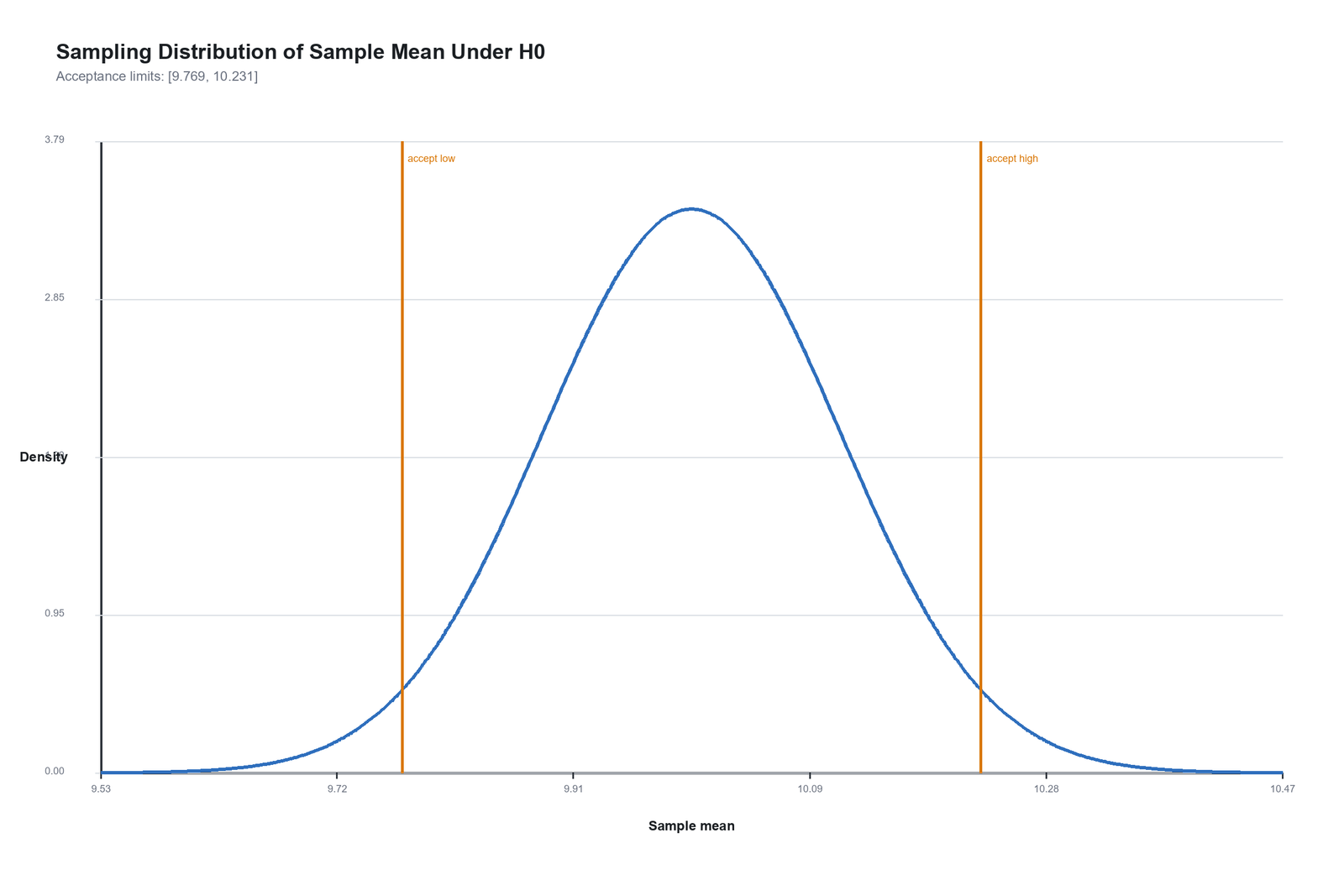
The R sampling distribution chart shows the same null-hypothesis acceptance region. The acceptance limits are [9.769, 10.231]. Under H0, sample means inside this interval would be considered ordinary at the displayed decision level.
The observed mean of 11.906 is far above this region. This means the observed mean is not consistent with the null hypothesis mean of 10.
The R chart validates the same decision: the null hypothesis should be rejected because the observed mean lies far outside the expected range under H0.
5. R Chart: Z Statistic on the Standard Normal Curve
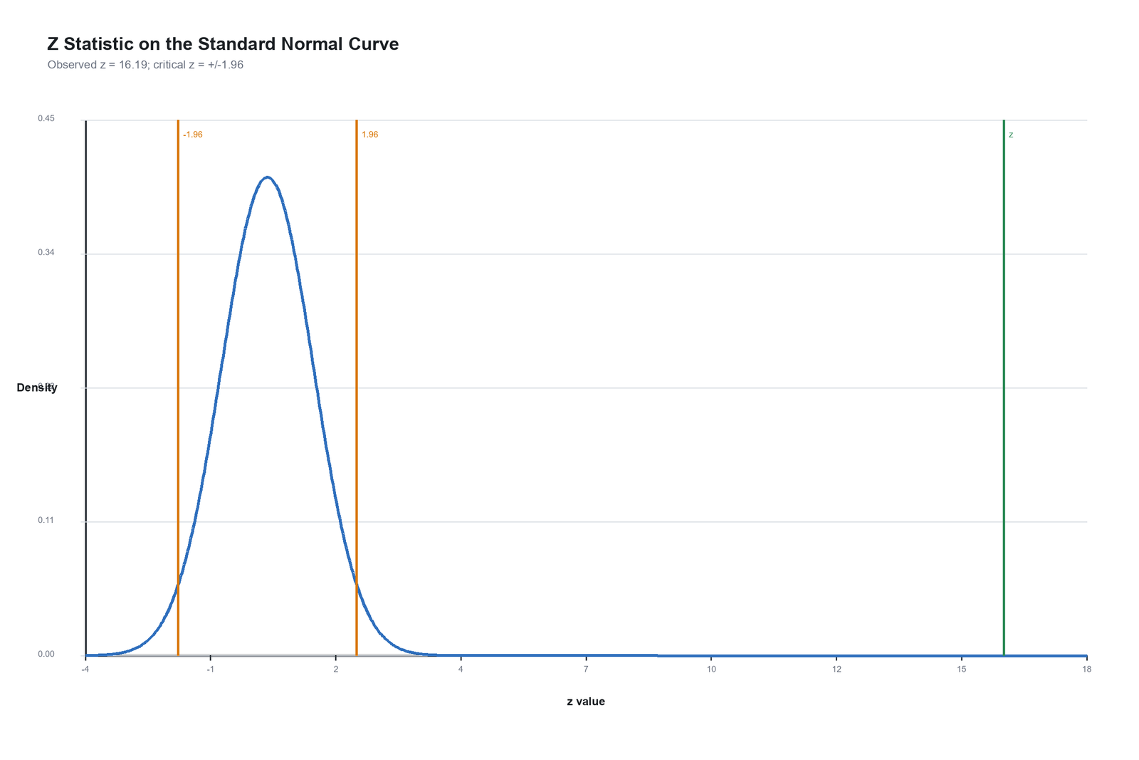
The R z-curve chart shows z = 16.19 on the standard normal curve. The critical values are ±1.96. The observed z value is far beyond the right-side critical boundary.
This confirms the final test decision. A z statistic this large indicates that the observed mean is extremely far from the hypothesized mean in standardized units.
The R chart supports reporting the result as statistically significant with p < .001.
6. R Chart: Confidence Interval for Population Mean
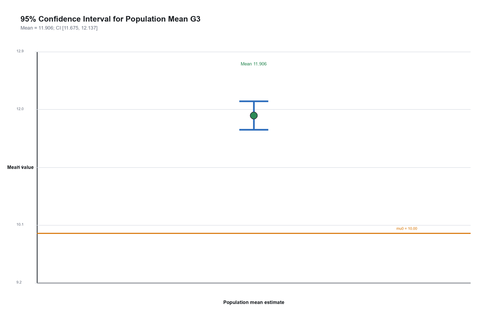
The R confidence interval chart confirms the interval [11.675, 12.137]. The observed mean is 11.906.
The hypothesized mean of 10.000 is not inside the interval. Therefore, the interval-based decision agrees with the z-test decision.
This chart helps explain the practical size of the result. The estimated population mean is above 10 by a clear margin.
7. R Chart: Mean G3 by School
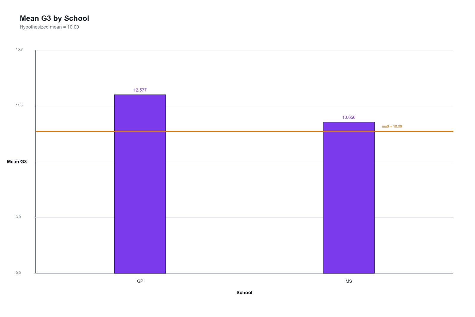
The R school chart confirms the same descriptive school means: GP = 12.577 and MS = 10.650. Both school means are above the hypothesized mean line of 10.000.
This chart helps readers understand the overall observed mean. The GP group has a higher average, while the MS group is closer to the null benchmark but still above it.
The school chart is descriptive context. A formal school comparison requires a two-sample mean test, not this one-sample population mean z test.
Overall Interpretation of All SPSS, Python and R Images
All image sets tell the same statistical story. The distribution images show that the observed mean is above the hypothesized mean. The mean-comparison images show 11.906 versus 10.000. The difference images show 1.906. The sampling-distribution images show acceptance limits of [9.769, 10.231], while the observed mean is far above that range. The z-curve images show z = 16.19, far beyond ±1.96. The confidence interval images show [11.675, 12.137], entirely above 10.000.
| Image type | Main message | How it supports the test |
|---|---|---|
| Distribution images | Observed mean = 11.906 is above μ0 = 10.000 | Shows the raw data context for the test. |
| Hypothesized vs observed mean images | Observed mean is higher than hypothesized mean | Shows the central comparison visually. |
| Observed minus hypothesized images | Difference = 1.906 | Shows the numerator of the z statistic. |
| Sampling distribution under H0 images | Acceptance limits = [9.769, 10.231] | Shows the observed mean is outside the H0 range. |
| Z statistic curve images | Observed z = 16.19; critical z = ±1.96 | Shows the result is far into the rejection region. |
| Confidence interval images | 95% CI = [11.675, 12.137] | Shows the estimated population mean is above 10. |
| School mean images | GP = 12.577 and MS = 10.650 | Provides descriptive subgroup context. |
The final decision is consistent across SPSS, Python and R: reject the null hypothesis. The observed G3 mean is significantly different from the hypothesized population mean of 10.000, and the direction shows that the observed mean is higher.
How to Run Z Test for Population Mean in SPSS, Python, R and Excel
SPSS Method
SPSS can calculate the observed mean and then compute the z statistic manually using the hypothesized mean and standard error. The structure below matches the logic of the image output.
* Z Test for Population Mean in SPSS.
* Test whether mean G3 differs from hypothesized mean 10.000.

DESCRIPTIVES VARIABLES=G3
  /STATISTICS=MEAN STDDEV MIN MAX.

* Enter exact values from the image output.
INPUT PROGRAM.
DATA LIST FREE /observed_mean hypothesized_mean z_value ci_low ci_high.
BEGIN DATA
11.906 10.000 16.19 11.675 12.137
END DATA.
END FILE.
END INPUT PROGRAM.

COMPUTE mean_difference = observed_mean - hypothesized_mean.
COMPUTE decision = (ABS(z_value) > 1.96).
EXECUTE.

FORMATS observed_mean hypothesized_mean mean_difference z_value ci_low ci_high (F10.3).
LIST.
Python Method
Python can reproduce the decision using the exact image-output values.
import math

observed_mean = 11.906
hypothesized_mean = 10.000
z_value = 16.19
ci_low = 11.675
ci_high = 12.137

difference = observed_mean - hypothesized_mean
p_value_two_tailed = math.erfc(abs(z_value) / math.sqrt(2))
decision = "Reject H0" if abs(z_value) > 1.96 else "Fail to reject H0"

print("Observed mean:", observed_mean)
print("Hypothesized mean:", hypothesized_mean)
print("Difference:", difference)
print("z:", z_value)
print("p-value:", p_value_two_tailed)
print("95% CI:", ci_low, ci_high)
print("Decision:", decision)
R Method
R can calculate the same decision using the exact values shown in the output charts.
observed_mean <- 11.906
hypothesized_mean <- 10.000
z_value <- 16.19
ci_low <- 11.675
ci_high <- 12.137

difference <- observed_mean - hypothesized_mean
p_value_two_tailed <- 2 * (1 - pnorm(abs(z_value)))
decision <- ifelse(abs(z_value) > 1.96, "Reject H0", "Fail to reject H0")

data.frame(
  observed_mean = observed_mean,
  hypothesized_mean = hypothesized_mean,
  difference = difference,
  z_value = z_value,
  p_value = p_value_two_tailed,
  ci_low = ci_low,
  ci_high = ci_high,
  decision = decision
)
Excel Method
Excel can calculate the same decision using ordinary formulas. Enter the exact output values into cells and calculate the difference, p-value and decision.
| Excel item | Formula or value | Purpose |
|---|---|---|
| Observed mean | 11.906 | Stores the observed G3 mean. |
| Hypothesized mean | 10.000 | Stores μ0. |
| Difference | =observed_mean_cell-hypothesized_mean_cell | Calculates observed minus hypothesized mean. |
| Z statistic | 16.19 | Stores the observed z statistic from the output. |
| Two-tailed p-value | =2*(1-NORM.S.DIST(ABS(z_cell),TRUE)) | Calculates the p-value from z. |
| Decision | =IF(ABS(z_cell)>1.96,"Reject H0","Fail to reject H0") | Applies the α = .05 two-tailed decision rule. |
| CI lower | 11.675 | Lower confidence bound. |
| CI upper | 12.137 | Upper confidence bound. |
How to Report the Z Test for Population Mean
A complete report should include the hypothesized mean, observed mean, mean difference, z statistic, p-value decision, confidence interval and conclusion.
APA-style report: A z test for population mean was conducted to determine whether the mean G3 final grade differed from 10.000. The observed sample mean was 11.906, giving an observed-minus-hypothesized difference of 1.906. The result was statistically significant, z = 16.19, p < .001, 95% CI [11.675, 12.137]. Therefore, the null hypothesis was rejected. The data provide strong evidence that the population mean G3 final grade is higher than 10.
In plain language, the sample average G3 score is about 1.906 grade points higher than the hypothesized benchmark. The estimated population mean is likely between 11.675 and 12.137, which is clearly above 10.
Common Mistakes in Z Test for Population Mean
1. Calling this a difference-between-two-means test
This image set tests one observed mean against one hypothesized mean. A difference-between-two-means test compares two independent group means. If the question is GP versus MS, use a Two Sample Z Test.
2. Confusing the observed mean and hypothesized mean
The hypothesized mean is 10.000. The observed mean is 11.906. The difference is 1.906.
3. Ignoring the confidence interval
The 95% confidence interval is [11.675, 12.137]. Because it does not include 10, it supports rejecting the null hypothesis.
4. Reporting p = .000
Do not report p = .000. For an extremely small p-value, write p < .001.
5. Using a proportion test for a mean
This is a mean-based test. If the outcome is pass/fail, use a proportion test such as the One Proportion Z Test.
6. Ignoring the z-test assumptions
A formal z test requires an appropriate standard error and an approximately normal sampling distribution. If the population standard deviation is unknown, a t test may be more appropriate.
FAQs About Z Test for Population Mean
What is a Z Test for Population Mean?
A Z Test for Population Mean is a hypothesis test used to compare one observed sample mean with one hypothesized population mean.
What is the formula for Z Test for Population Mean?
The formula is z = (x̄ − μ0) / SE, where x̄ is the observed sample mean, μ0 is the hypothesized mean and SE is the standard error.
What was the result in this example?
The hypothesized mean was 10.000, the observed mean was 11.906, the difference was 1.906, the observed z statistic was 16.19 and the 95% confidence interval was [11.675, 12.137]. The null hypothesis was rejected.
What does the confidence interval mean?
The confidence interval [11.675, 12.137] means the population mean G3 score is estimated to be between 11.675 and 12.137. Since 10.000 is not inside the interval, the null mean is not supported.
When should I use Z Test for Population Mean?
Use it when comparing one numeric sample mean with one hypothesized population mean, especially when the standard error is known or a valid z-test workflow is being used.
Is Z Test for Population Mean the same as One Sample Z Test?
Yes, in many practical guides, a z test for population mean is described as a one sample z test for a population mean.
Is this the same as Z Test for Difference Between Means?
No. This test compares one observed mean with one hypothesized mean. A z test for difference between means compares two independent group means.
Can I run Z Test for Population Mean in Excel?
Yes. Excel can calculate the difference, z statistic, p-value and decision using formulas such as subtraction, ABS and NORM.S.DIST.
Should I use a t test instead?
Use a one-sample t test when the population standard deviation is unknown and uncertainty must be estimated from the sample standard deviation.
How do I report a very small p-value?
Report very small p-values as p < .001 instead of p = .000.

