
Welch implementation with equal_var=False
Unequal-Variance T-Test in SciPy, R & SPSS
Run the unequal-variance Welch t-test with scipy.stats.ttest_ind(..., equal_var=False), R t.test(..., var.equal=FALSE), or the SPSS “Equal variances not assumed” row. For the mathematical derivation, use the complete Welch’s t-test formula guide.
Quick Answer: How to Run the Unequal-Variance T-Test
The worked T Test for Unequal Variances compares mean G3 final grade between GP and MS. GP has n = 423, mean 12.5768, standard deviation 2.6256, and variance 6.8940. MS has n = 226, mean 10.6504, standard deviation 3.8340, and variance 14.6995. Since MS has a larger variance, the unequal-variance Welch method is appropriate.
The observed mean difference is 1.9264 in favor of GP. The Welch standard error is approximately 0.2852. The Welch t statistic is approximately 6.7545, with adjusted degrees of freedom approximately 340.49, and the p value is p < .001. The 95% confidence interval for the mean difference is approximately 1.3654 to 2.4874. Since the interval is fully above zero, GP students have significantly higher average G3 scores than MS students.
Final interpretation: The T Test for Unequal Variances shows that GP students scored significantly higher on G3 than MS students. The Welch test is appropriate because group variances are unequal, the confidence interval is fully above zero, and the p value is below .001.
Important reporting point: Welch’s t test does not use pooled variance. It uses separate variance components for each group and adjusts the degrees of freedom, which is why Welch df is often decimal.
Table of Contents
- What Is a T Test for Unequal Variances?
- T Test for Unequal Variances Formula
- Null and Alternative Hypothesis
- Dataset and Group Variables Used
- SPSS Output Interpretation
- Python Chart-by-Chart Interpretation
- R Chart-by-Chart Validation
- SPSS, R, Python and Excel Workflows
- Code Blocks for T Test for Unequal Variances
- APA Reporting Wording
- Common Mistakes
- When to Use T Test for Unequal Variances
- Downloads and Resources
- Related Guides
- FAQs
What Is a T Test for Unequal Variances?
A T Test for Unequal Variances is an independent samples t test used when the two groups do not have similar variances. It is usually called Welch’s t test. In SPSS-style output, it appears as the Equal variances not assumed row.
The purpose of this test is the same as the ordinary independent samples t test: compare two group means. The difference is how the standard error and degrees of freedom are calculated. Instead of pooling the two variances into one shared estimate, Welch’s method keeps the variance components separate.
In this example, GP and MS are independent school groups. GP has a smaller variance, while MS has a larger variance. Because the spread is not the same across groups, Welch’s method is safer than the equal-variances-assumed Student’s t test.
Simple definition: A T Test for Unequal Variances compares two independent group means without assuming that the two groups have equal variances. It is the preferred t test when group spreads are different.
T Test for Unequal Variances should be interpreted with group means, group variances, variance ratio, Welch standard error, Welch degrees of freedom, t statistic, confidence interval, p value and effect size. Related guides include T Test Assumptions, Levene Test, Standard Deviation, Standard Error, Confidence Interval, P Value, and Effect Size.
T Test for Unequal Variances Formula
The Welch T Test for Unequal Variances compares the difference between two group means with a standard error that keeps group variances separate:
The observed mean difference in this example is:
The Welch standard error is:
Welch degrees of freedom are adjusted using the Welch-Satterthwaite equation:
| Symbol | Meaning | Value in This Example |
|---|---|---|
| x̄GP | Mean of GP group | 12.5768 |
| x̄MS | Mean of MS group | 10.6504 |
| nGP | GP sample size | 423 |
| nMS | MS sample size | 226 |
| sGP | GP standard deviation | 2.6256 |
| sMS | MS standard deviation | 3.8340 |
| sGP2/nGP | GP standard error component | ≈ 0.0163 |
| sMS2/nMS | MS standard error component | ≈ 0.0650 |
| SEWelch | Welch standard error | ≈ 0.2852 |
| t | Welch test statistic | ≈ 6.7545 |
| df | Welch adjusted degrees of freedom | ≈ 340.49 |
Threshold rule: If the Welch confidence interval for the mean difference does not include zero, the two group means are significantly different. In this example, the interval is fully above zero, so GP has a significantly higher mean G3 score than MS.
Null and Alternative Hypothesis for T Test for Unequal Variances
The T Test for Unequal Variances tests whether two independent population means are equal while allowing the population variances to be unequal.
| Statement | Hypothesis | Meaning |
|---|---|---|
| Null hypothesis | H0: μGP = μMS | The population mean G3 score is equal for GP and MS. |
| Alternative hypothesis | H1: μGP ≠ μMS | The population mean G3 score differs between GP and MS. |
| Observed direction | x̄GP − x̄MS = 1.9264 | The observed mean is higher for GP than MS. |
Decision for this example: The null hypothesis is rejected because the Welch t statistic is large, the p value is below .001, and the 95% confidence interval for GP − MS is fully above zero.
Dataset and Group Variables Used
The worked example uses a student performance dataset. The outcome variable is G3 final grade. The grouping variable is school, with two independent groups: GP and MS. The unequal-variance workflow compares group variances, group means, Welch standard error components, confidence intervals, t distributions and SPSS-style output tables.
| Variable or Value | Role | Why It Matters for Unequal Variances |
|---|---|---|
| G3 | Dependent variable | The final grade whose mean is compared between groups. |
| school | Grouping variable | Defines GP and MS as independent groups. |
| GP | Group 1 | n = 423, mean = 12.5768, variance = 6.8940. |
| MS | Group 2 | n = 226, mean = 10.6504, variance = 14.6995. |
| Welch method | Unequal-variance solution | Uses separate variance components and adjusted degrees of freedom. |
Before interpreting a T Test for Unequal Variances, examine group statistics, variance comparison, standard deviation comparison, distribution by group and the difference between equal-variance and Welch results. Useful supporting guides include T Test Assumptions, Levene Test, Standard Deviation, Standard Error, and Confidence Interval.
SPSS Output Interpretation for T Test for Unequal Variances
In SPSS, the T Test for Unequal Variances is interpreted from the Equal variances not assumed row of the Independent Samples Test table. This is the Welch-style row. It is preferred when Levene’s test, variance ratio, standard deviation comparison or visual spread checks show that the equal-variance assumption is questionable.
SPSS Group Statistics
| SPSS Output Item | GP | MS | Interpretation |
|---|---|---|---|
| N | 423 | 226 | Both groups are large, but the sample sizes are unequal. |
| Mean | 12.5768 | 10.6504 | GP has the higher average G3 score. |
| Std. Deviation | 2.6256 | 3.8340 | MS has greater spread than GP. |
| Variance | 6.8940 | 14.6995 | The MS variance is more than twice the GP variance. |
| Std. Error Mean | ≈ 0.1277 | ≈ 0.2550 | The MS mean is less precise because MS has greater spread and fewer observations. |
SPSS Unequal Variance Summary
| Output Item | Value | Interpretation |
|---|---|---|
| Variance ratio | 2.1322 | MS variance is about 2.13 times GP variance. |
| Larger variance group | MS | MS contributes more to the Welch standard error. |
| Recommended method | Welch t test | Welch is safer when variances are unequal. |
| Comparison order | GP − MS | A positive difference means GP has the higher mean. |
SPSS Equal Variances Not Assumed T Test
| SPSS Output Item | Value | Interpretation |
|---|---|---|
| Assumption row | Equal variances not assumed | This is the Welch t-test row. |
| Mean difference | 1.9264 | GP mean is 1.9264 points higher than MS mean. |
| Welch standard error | ≈ 0.2852 | The standard error uses separate group variances. |
| t | ≈ 6.7545 | The difference is large relative to the Welch standard error. |
| df | ≈ 340.49 | The degrees of freedom are adjusted and therefore decimal. |
| Sig. (2-tailed) | < .001 | The difference between group means is statistically significant. |
| 95% CI Lower | ≈ 1.3654 | The lower bound is above zero. |
| 95% CI Upper | ≈ 2.4874 | The upper bound remains positive. |
SPSS interpretation summary: The equal variances not assumed row showed that GP students had significantly higher G3 scores than MS students, t(340.49) ≈ 6.7545, p < .001. The mean difference was 1.9264, with a 95% confidence interval of approximately [1.3654, 2.4874]. Because MS had the larger variance, Welch’s unequal-variance t test is the safer interpretation.
Python Chart-by-Chart Interpretation
The Python charts below show the complete T Test for Unequal Variances workflow. They include group variance comparison, group means, Welch standard error components, Welch confidence interval, Welch t distribution, group distributions, Welch versus equal-variance p value comparison and SPSS-style tables.
Python Chart 1: Group Variance Comparison for Unequal Variances
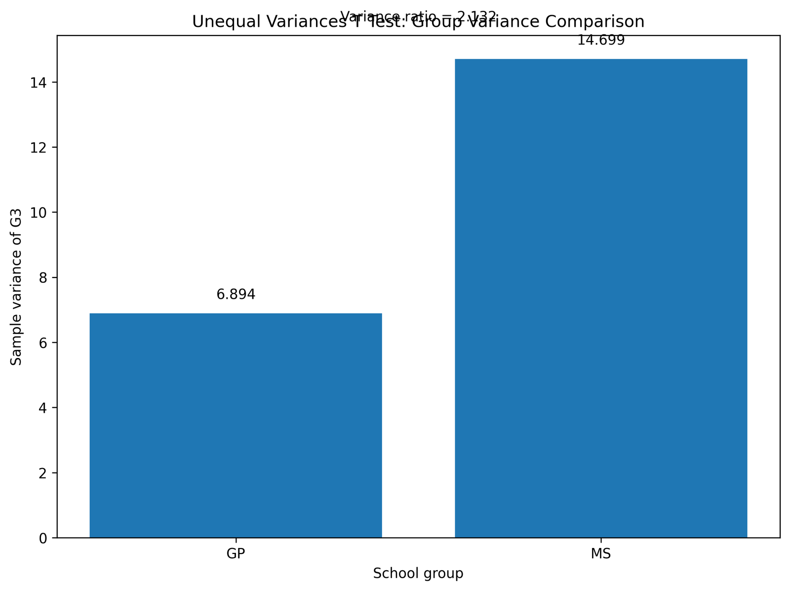
This chart compares the two group variances. GP has variance 6.8940, while MS has variance 14.6995. MS has the larger spread.
The chart explains why the unequal-variance t test is appropriate. When group variances differ, Welch’s method avoids forcing the groups into one pooled variance estimate.
Python Chart 2: Group Means for Unequal Variances
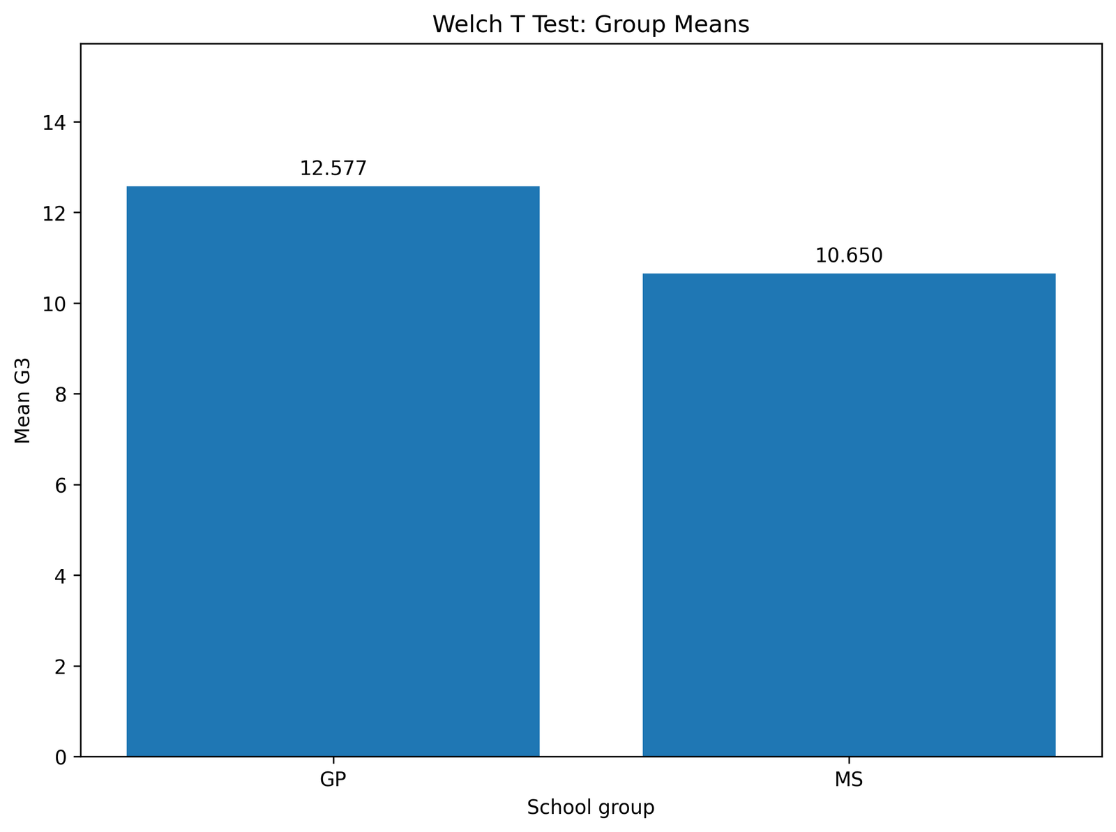
This chart shows the group means being compared. GP has mean 12.5768, while MS has mean 10.6504. The observed difference is positive and favors GP.
The chart is useful because the t test begins with the group mean difference. Welch’s method then asks whether that difference is large relative to the unequal-variance standard error.
Python Chart 3: Welch Standard Error Components
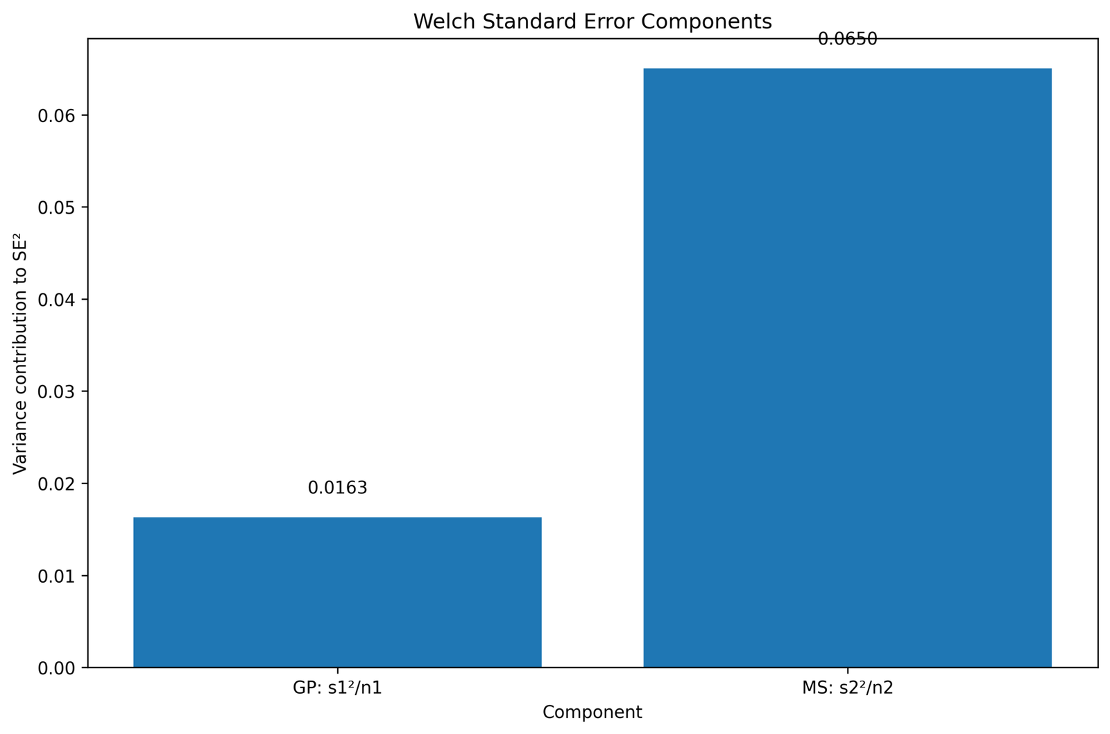
This chart explains the key calculation behind Welch’s test. The GP standard error component is approximately 0.0163, while the MS component is approximately 0.0650. MS contributes more uncertainty because it has a larger variance and smaller sample size.
This chart is central to the unequal-variance method. It shows that Welch’s test does not hide variance differences inside a pooled estimate.
Python Chart 4: Welch Confidence Interval for Mean Difference
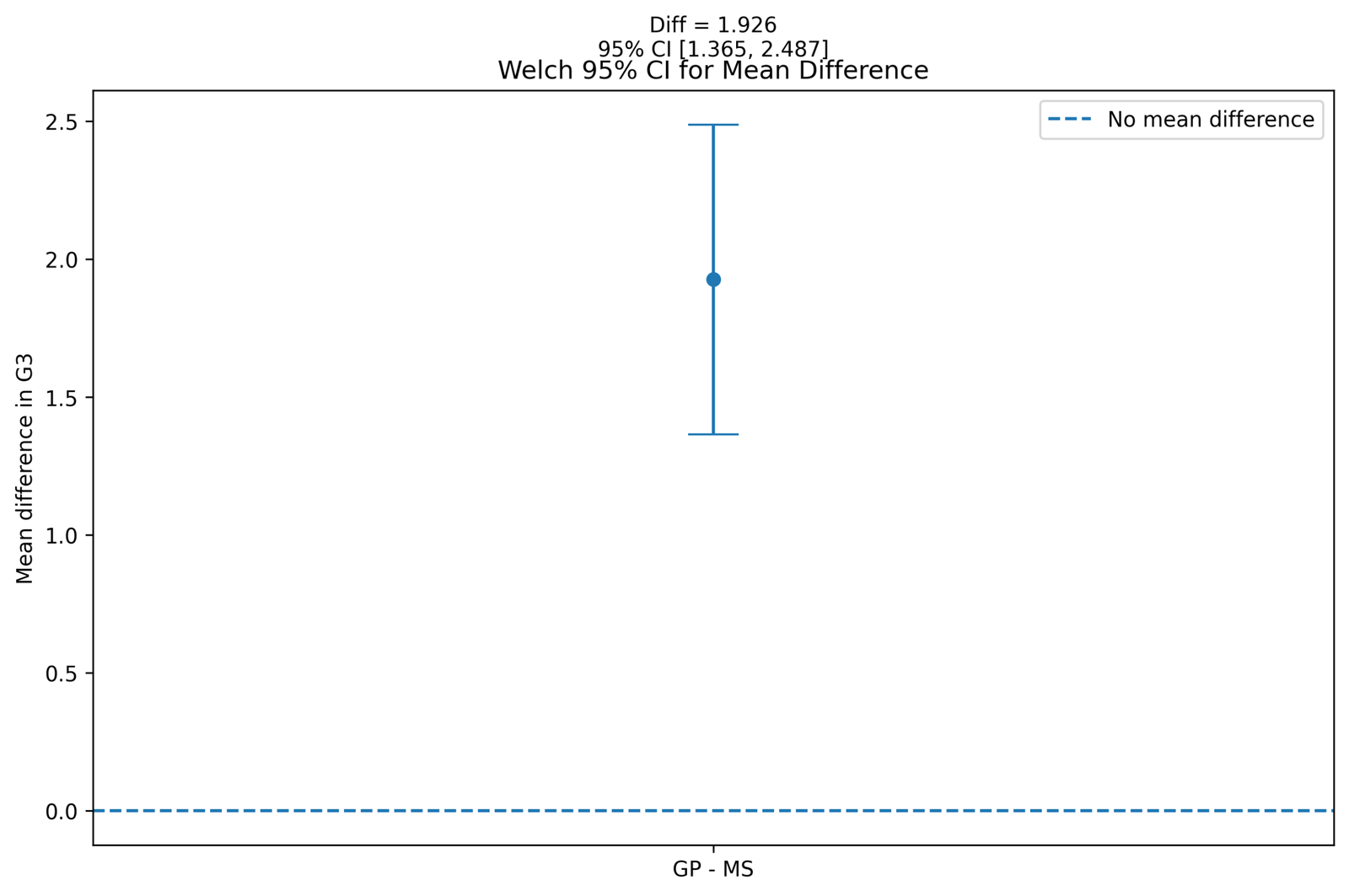
This chart shows the confidence interval for the mean difference under Welch’s method. The interval is approximately 1.3654 to 2.4874, and it is fully above zero.
Because zero is not inside the interval, the result is statistically significant. The positive interval also shows that the direction favors GP.
Python Chart 5: Welch T Distribution for Unequal Variances
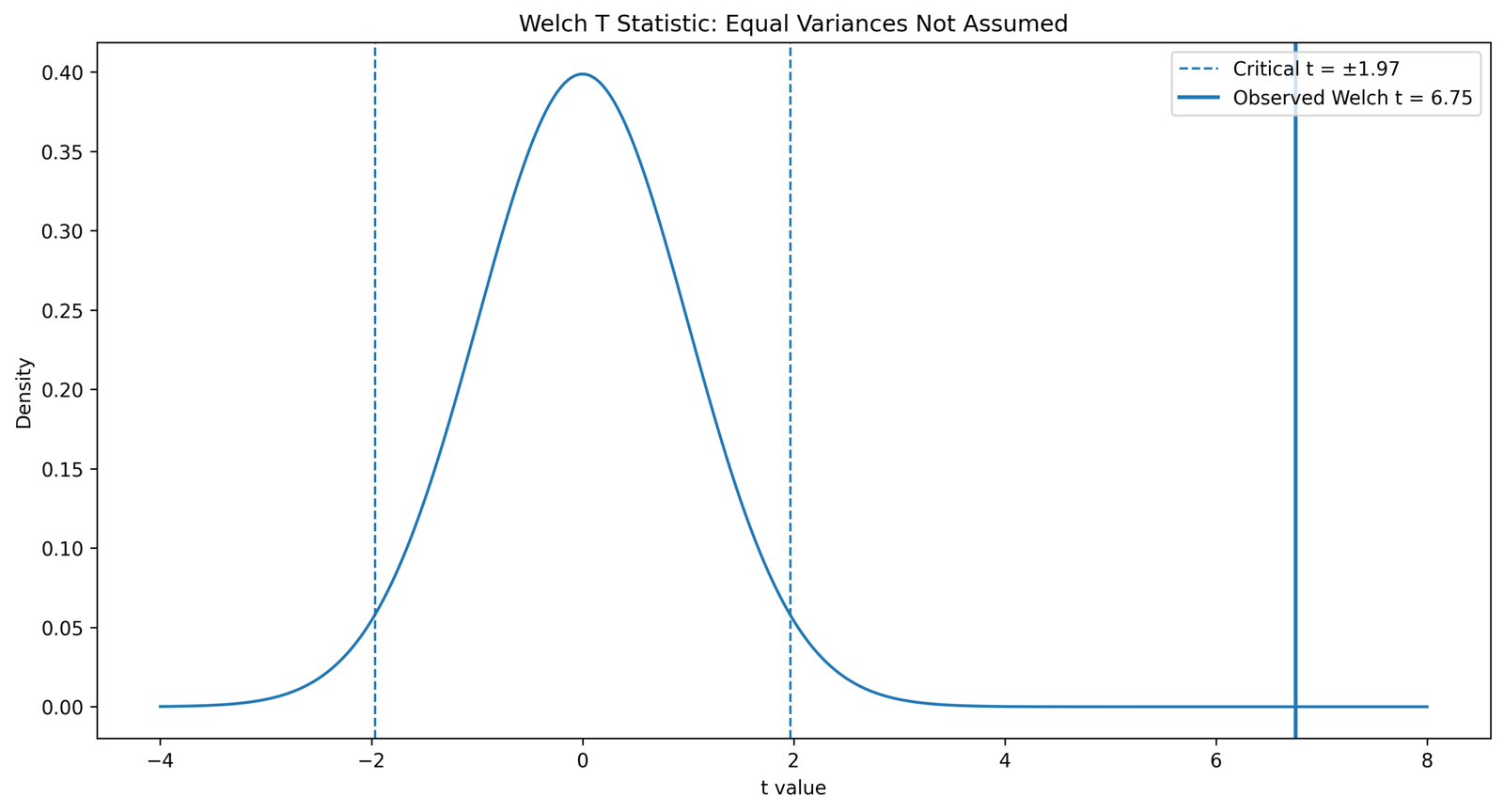
This chart places the Welch t statistic in the t-test decision framework. The observed statistic is approximately 6.7545, with adjusted degrees of freedom approximately 340.49.
The observed t statistic is far from zero, which explains why the p value is below .001. The decimal degrees of freedom are normal in Welch’s test.
Python Chart 6: Distribution by Group for Unequal Variances
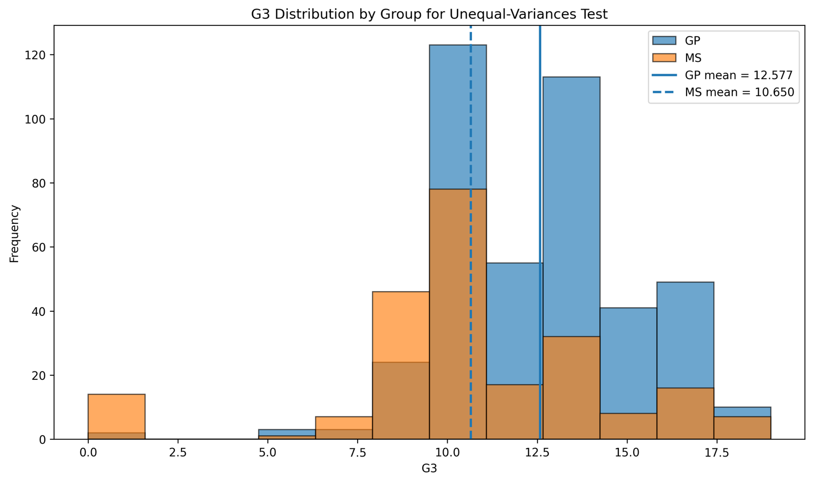
This distribution chart shows the raw score pattern behind the Welch test. GP is centered higher, while MS has a wider spread. This matches both the mean comparison and the variance comparison.
The chart supports the unequal-variance interpretation because the group distributions do not show identical spread.
Python Chart 7: Welch vs Equal Variance P Value Comparison
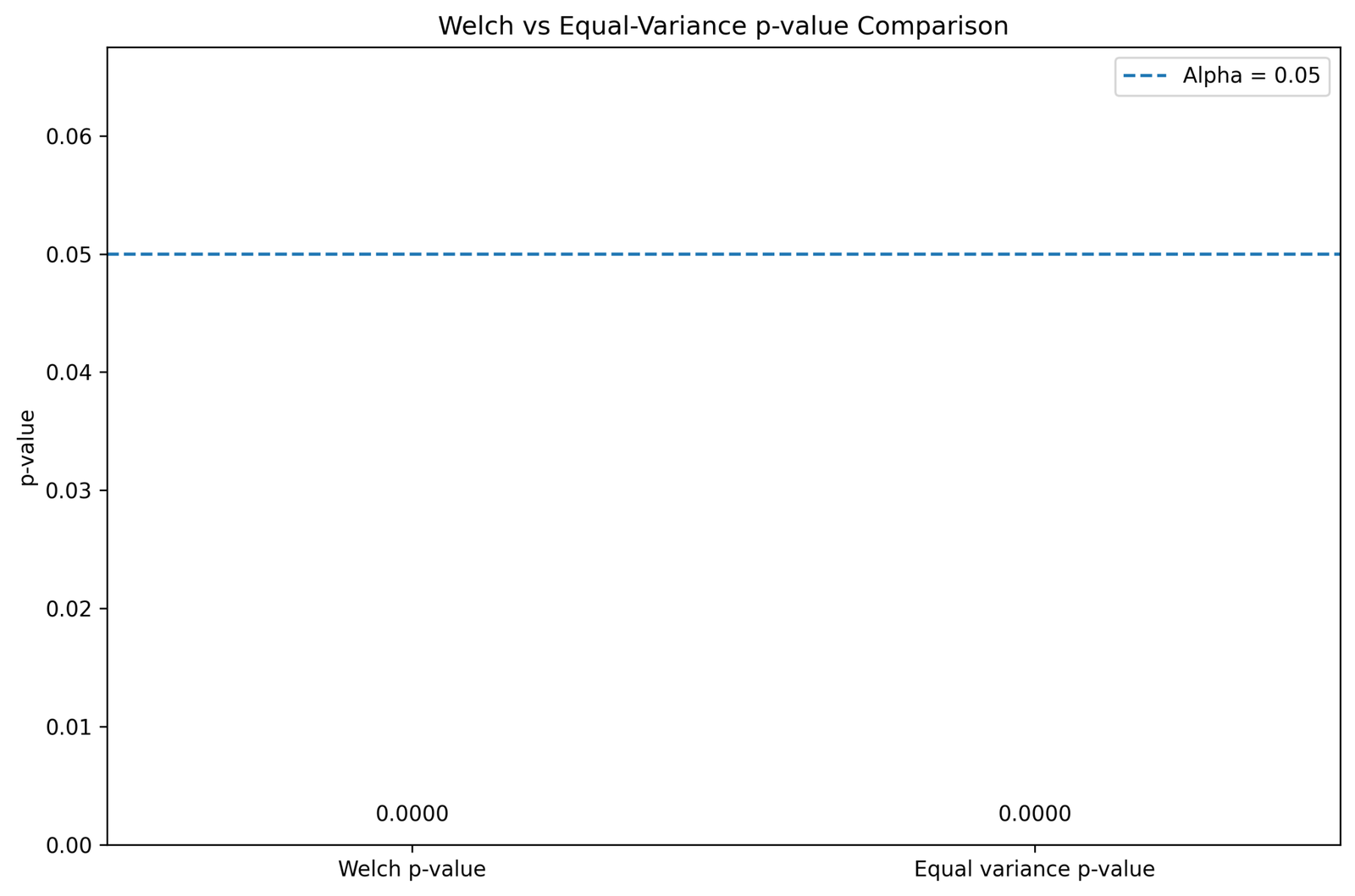
This chart compares the p value from Welch’s unequal-variance method with the p value from the equal-variance method. In this dataset, both methods lead to a significant conclusion.
The value of Welch’s test is not that it always changes the conclusion. Its value is that it protects the analysis when the equal variance assumption is questionable.
Python Chart 8: Group Statistics Table
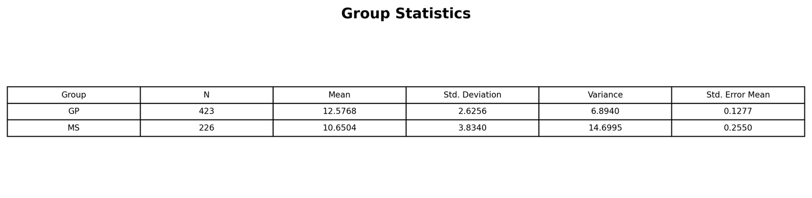
This table provides the descriptive statistics behind the Welch test. GP has higher mean and lower variance, while MS has lower mean and higher variance.
The table is important because it explains both parts of the result: the mean difference and the unequal variance condition.
Python Chart 9: Unequal Variance Summary Table
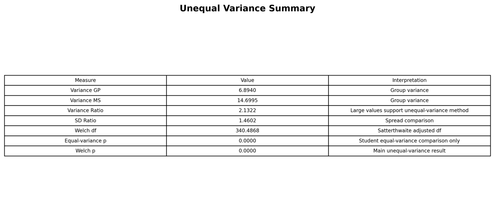
This summary table explains why the unequal-variance route is selected. It identifies the larger variance group, variance ratio and Welch method recommendation.
This table is useful for reporting because it connects assumption checking with the final choice of t-test row.
Python Chart 10: Independent Samples Unequal Variances T Test Table
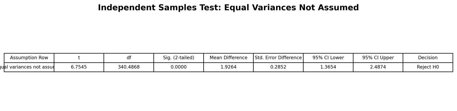
This is the main unequal-variance t-test table. It reports the Welch mean difference, standard error, t statistic, adjusted degrees of freedom, p value and confidence interval.
The table supports the final conclusion that GP has a significantly higher mean G3 score than MS under the equal variances not assumed row.
R Chart-by-Chart Validation
The R charts validate the Python and SPSS-style conclusions using a separate workflow. The same pattern appears: MS has larger variance, GP has higher mean, Welch standard error uses separate components, the confidence interval excludes zero, the t statistic is significant, and the unequal-variance tables support the Welch interpretation.
R Chart 1: Group Variance Comparison for Unequal Variances
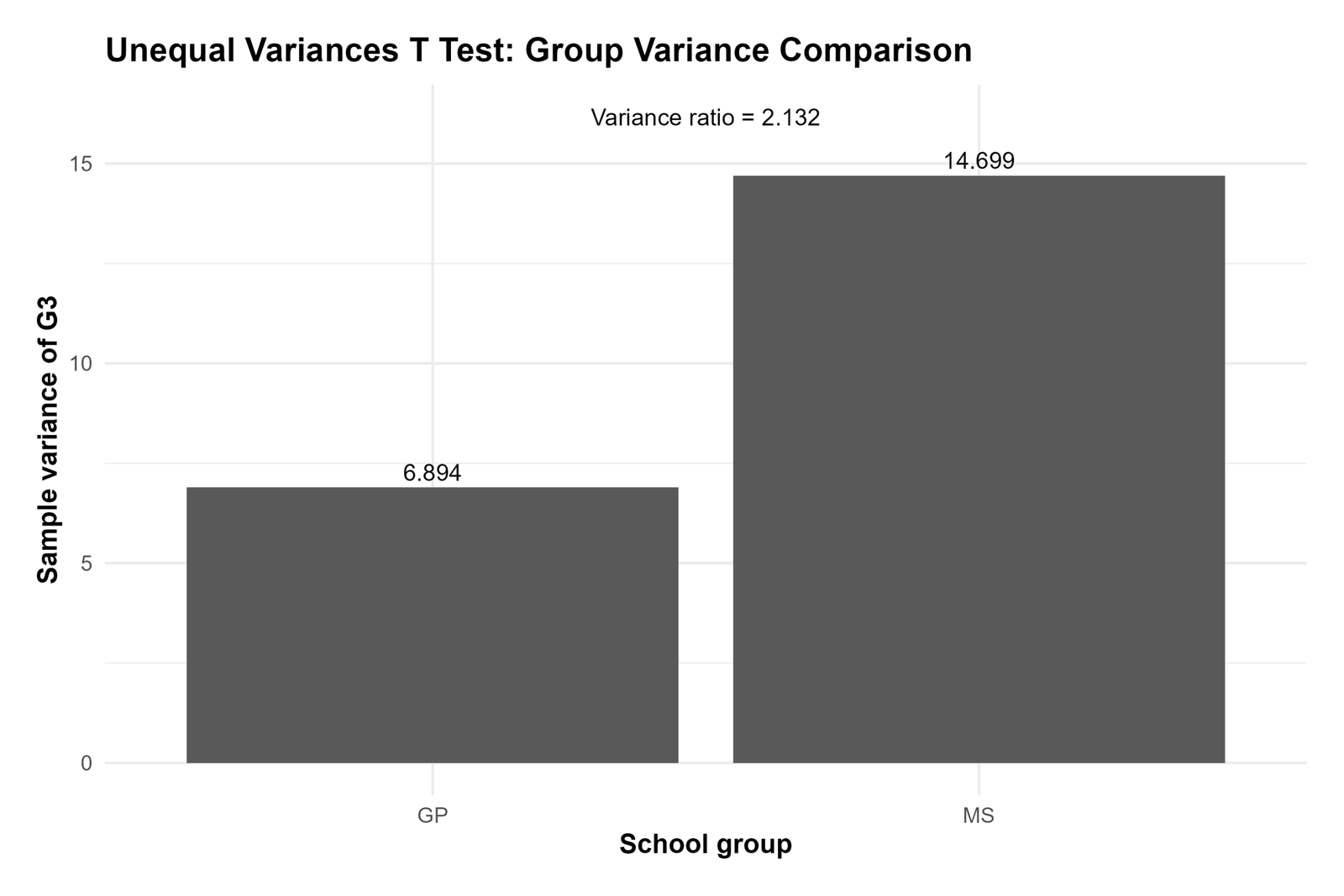
The R variance chart confirms the Python result. MS has the larger variance, which supports using Welch’s unequal-variance t test.
This validation shows that the variance pattern is reproducible across software.
R Chart 2: Group Means for Unequal Variances
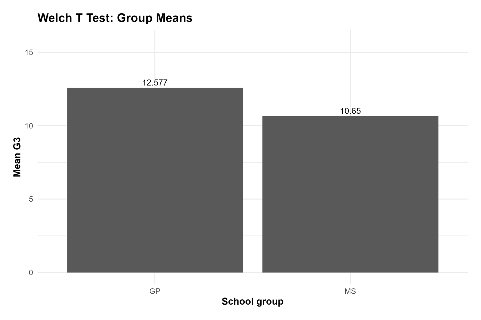
The R group means chart confirms that GP has the higher average G3 score. The observed mean difference is positive and matches the Python output.
This chart validates the direction of the final hypothesis-test result.
R Chart 3: Welch Standard Error Components
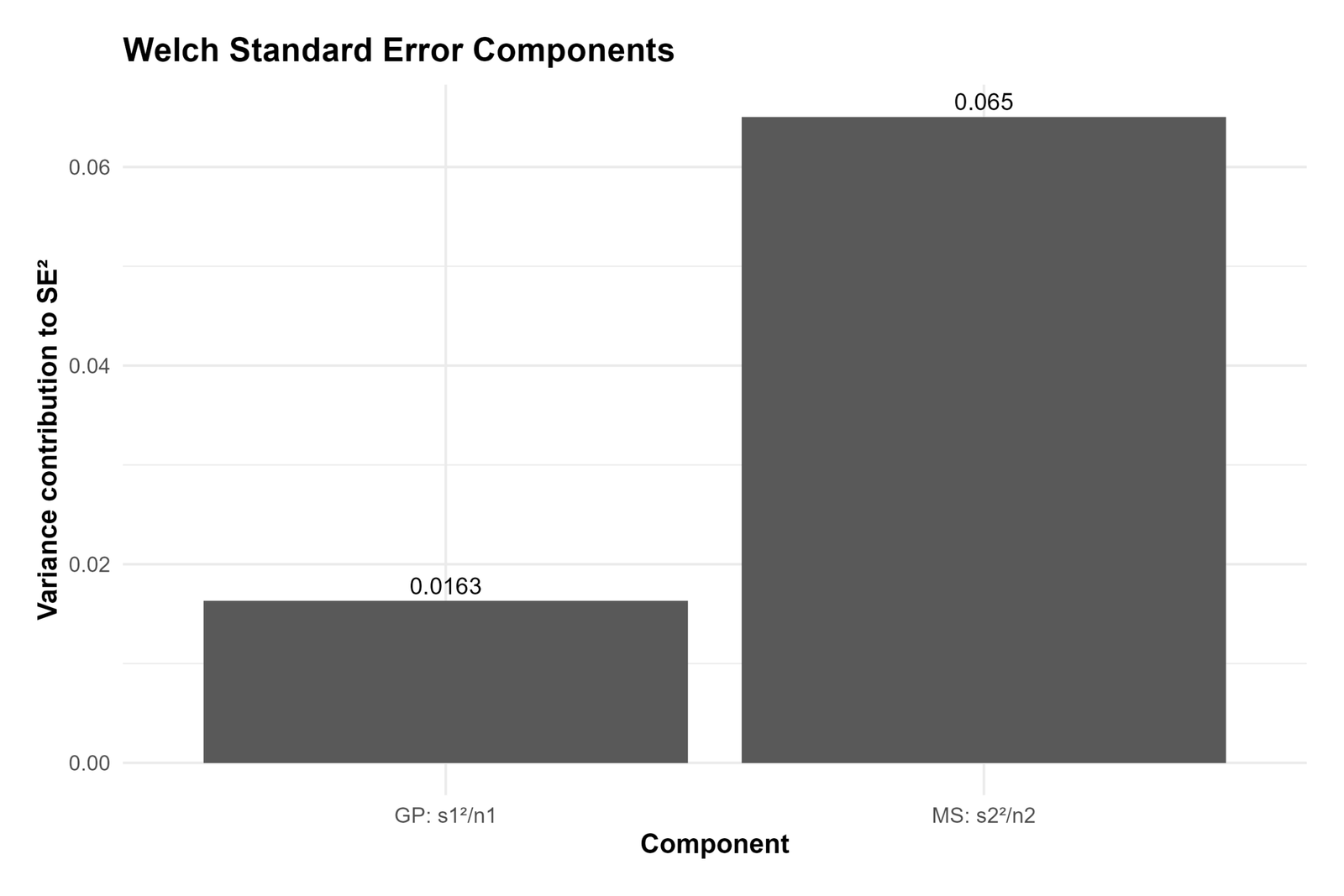
The R standard-error chart confirms the separate variance-component logic of Welch’s test. The MS component is larger because MS has greater variance and fewer observations.
This chart explains why Welch’s test is safer than pooling the variances.
R Chart 4: Welch Confidence Interval for Mean Difference
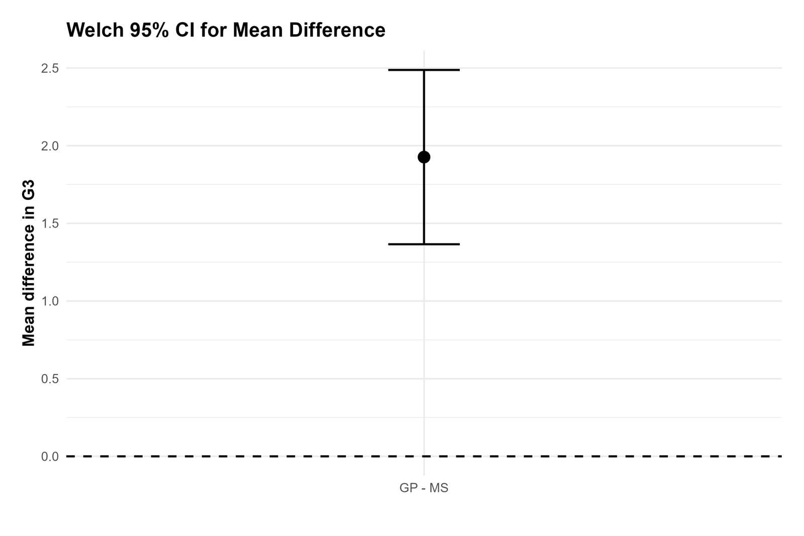
The R confidence interval chart confirms that the Welch confidence interval is fully above zero. The group difference is statistically significant and positive.
This chart supports the final conclusion that GP has the higher mean G3 score.
R Chart 5: Welch T Distribution for Unequal Variances
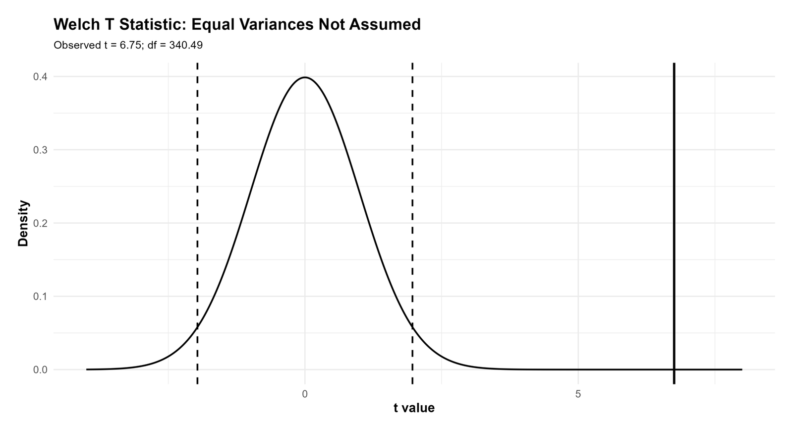
The R t-distribution chart validates the inferential result. The observed Welch t statistic is far from zero, so the p value is very small.
The chart helps readers understand why the null hypothesis of equal means is rejected.
R Chart 6: Distribution by Group for Unequal Variances
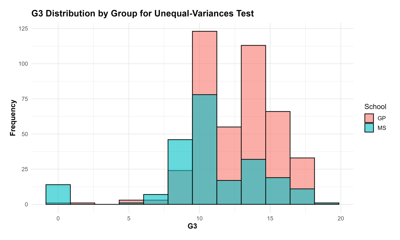
The R distribution chart confirms the group-level pattern. GP is centered higher, while MS has a wider distribution.
This visual supports both the mean-difference conclusion and the unequal-variance assumption decision.
R Chart 7: Welch vs Equal Variance P Value Comparison
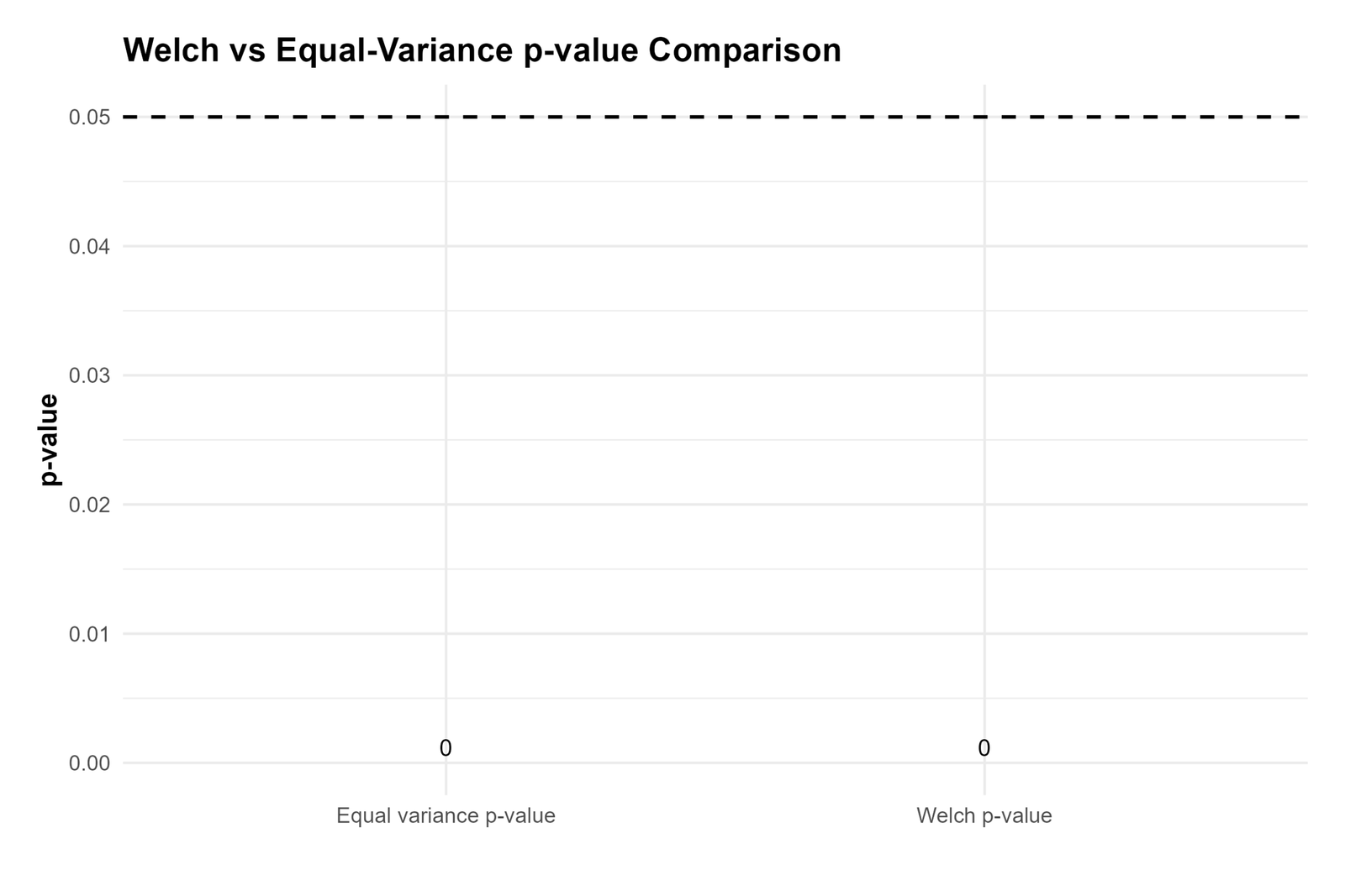
The R comparison chart confirms that both Welch and equal-variance approaches produce significant p values in this dataset.
However, Welch remains the better reporting choice when the variance assumption is questionable because it does not require equal variances.
R Chart 8: Group Statistics Table

The R group statistics table repeats the descriptive summary. GP has the higher mean and smaller variance, while MS has the lower mean and larger variance.
This table confirms the numerical basis for using Welch’s test.
R Chart 9: Unequal Variance Summary Table
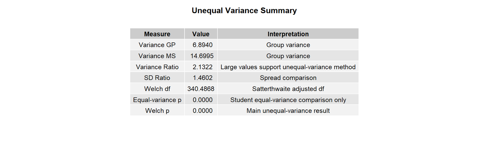
The R unequal-variance summary table confirms that the variance condition supports the Welch approach. It connects the assumption check with the final statistical method.
This table is useful for transparent reporting because it explains why the unequal-variance row is used.
R Chart 10: Independent Samples Unequal Variances T Test Table
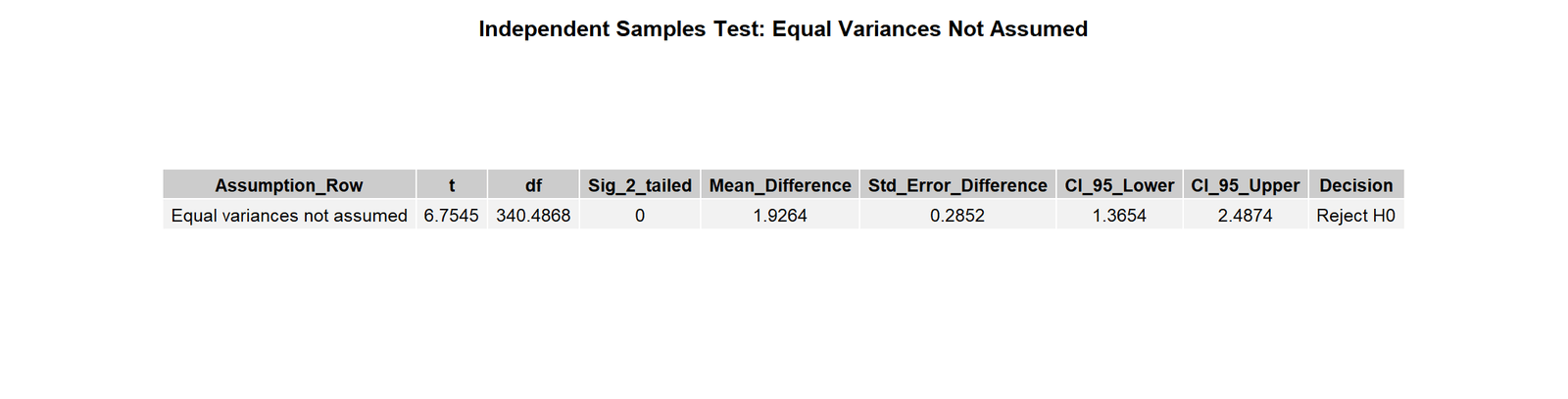
The R unequal-variance t-test table confirms the main inference. The Welch result is significant, the confidence interval is above zero, and the group mean difference favors GP.
This validates the final conclusion using a separate workflow.
Additional Output 1: Group Variance Comparison for Unequal Variances
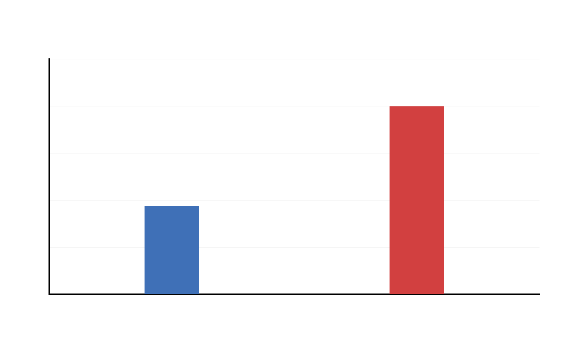
This additional output preserves the complete chart set and confirms that MS has the larger variance.
The repeated visual strengthens the assumption explanation for using Welch’s t test.
Additional Output 2: Group Means for Unequal Variances
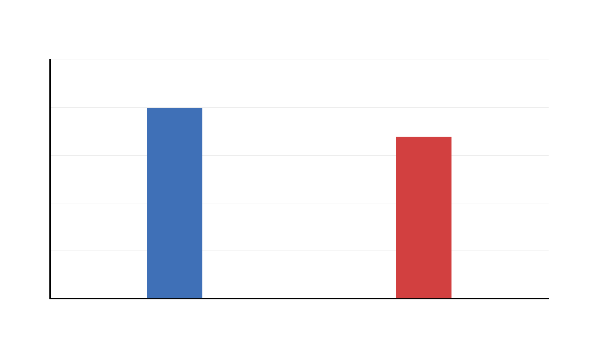
This additional group means chart confirms that GP has the higher average G3 score.
It supports the direction of the final Welch t-test result.
Additional Output 3: Welch Standard Error Components
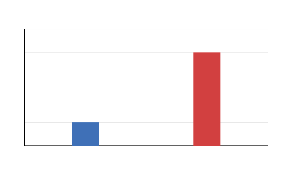
This additional standard-error chart repeats the main Welch calculation idea. The standard error is built from separate variance components.
This is the key difference between Welch’s t test and the equal-variances-assumed Student’s t test.
Additional Output 4: Welch Confidence Interval for Mean Difference
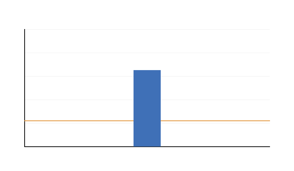
This additional confidence interval output confirms that the interval remains fully above zero.
The chart supports the conclusion that the group mean difference is statistically significant and positive.
Additional Output 5: Welch T Distribution for Unequal Variances
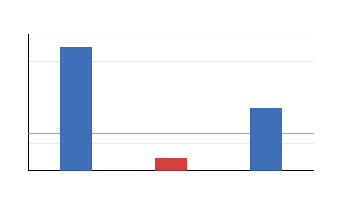
This additional t-distribution chart confirms the statistical decision. The observed Welch t statistic is far from zero.
The chart provides visual support for the small p value.
Additional Output 6: Distribution by Group for Unequal Variances
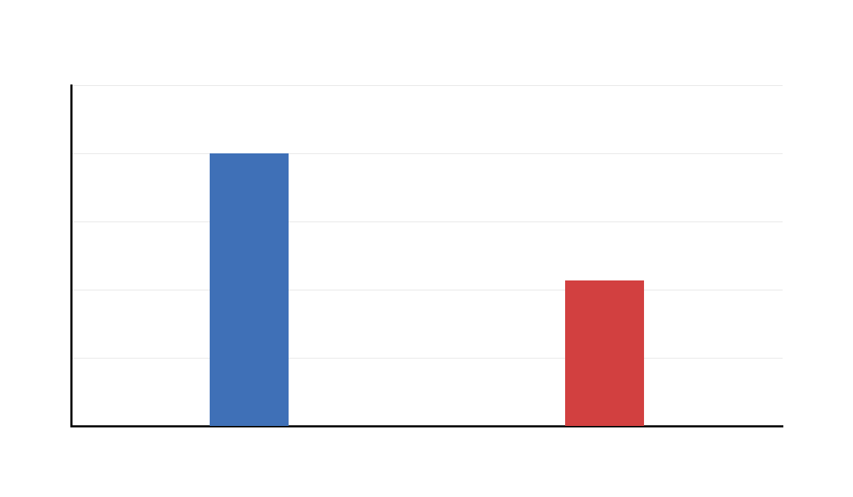
This additional distribution chart confirms the visible spread difference between GP and MS.
It supports the unequal-variance decision because group distributions do not have identical spread.
Additional Output 7: Welch vs Equal Variance P Value Comparison
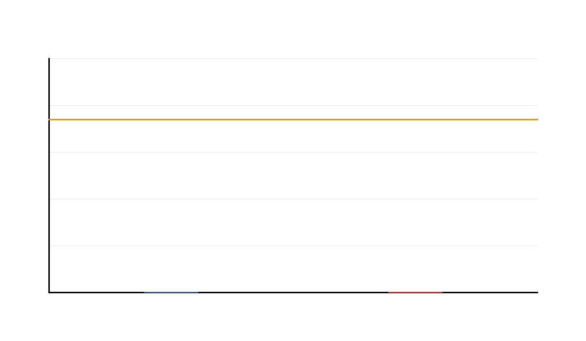
This additional p-value comparison chart confirms that the conclusion remains significant under both approaches.
The reason to prefer Welch is not only the p value; it is the safer assumption structure under unequal variances.
Additional Output 8: Group Statistics Table
This additional statistics table repeats the group sample size, mean, standard deviation, variance and standard error information.
It provides the numerical foundation for the Welch t-test result.
Additional Output 9: Unequal Variance Summary Table
This additional summary table confirms the unequal-variance context and the recommendation to use Welch’s method.
The table connects assumption evidence with the final test selection.
Additional Output 10: Independent Samples Unequal Variances T Test Table
This additional t-test table repeats the final Welch result. It confirms the adjusted degrees of freedom, mean difference, confidence interval and p value.
The output provides final evidence that GP has a significantly higher average G3 score than MS under the unequal-variance method.
SPSS, R, Python and Excel Workflows for T Test for Unequal Variances
The same T Test for Unequal Variances workflow can be reproduced in SPSS, R, Python and Excel. SPSS reports the unequal-variance result in the Equal variances not assumed row. R uses t.test(..., var.equal = FALSE). Python uses scipy.stats.ttest_ind(..., equal_var=False). Excel uses the Data Analysis ToolPak option t-Test: Two-Sample Assuming Unequal Variances.
SPSS Workflow
| Step | SPSS Menu or Syntax | Purpose |
|---|---|---|
| Open dataset | File > Open > Data | Load the clean dataset. |
| Run independent t test | Analyze > Compare Means > Independent-Samples T Test | Open the two-group mean comparison procedure. |
| Set test variable | Move G3 into Test Variable(s) | Choose final grade as the dependent variable. |
| Set grouping variable | Move school into Grouping Variable | Define GP and MS as the two groups. |
| Check equal variance | Read Levene’s Test or variance evidence | Decide whether equal variance is questionable. |
| Interpret Welch row | Equal variances not assumed | Report Welch t, adjusted df, p value and CI. |
| Export output | File > Export or OUTPUT EXPORT | Save a PDF for reporting and verification. |
R Workflow
| Step | R Action | Purpose |
|---|---|---|
| Read data | read.csv() | Load the dataset. |
| Select variables | G3 and school | Define dependent and grouping variables. |
| Check variances | var(), sd(), var.test() | Compare group spread. |
| Run Welch t test | t.test(G3 ~ school, data = df, var.equal = FALSE) | Run the unequal-variance independent samples t test. |
| Create charts | Variance bars, distributions and Welch CI charts | Visualize the unequal-variance result. |
Python Workflow
| Step | Python Action | Purpose |
|---|---|---|
| Read data | pandas.read_csv() | Load the dataset into a DataFrame. |
| Split groups | Filter G3 by school | Create GP and MS samples. |
| Compare variances | Calculate variances and variance ratio | Show why Welch is preferred. |
| Run Welch test | stats.ttest_ind(gp, ms, equal_var=False) | Calculate Welch t statistic and p value. |
| Calculate Welch CI | Manual Welch standard error and df formula | Report confidence interval for mean difference. |
Excel Workflow
| Excel Task | Formula or Tool | Purpose |
|---|---|---|
| Separate groups | Put GP and MS G3 values in two columns | Prepare independent group samples. |
| Calculate variances | =VAR.S(range) | Estimate each group variance. |
| Calculate variance ratio | =MAX(var1,var2)/MIN(var1,var2) | Screen unequal variance. |
| Run Welch test | Data Analysis ToolPak > t-Test: Two-Sample Assuming Unequal Variances | Run the unequal-variance t test. |
| Interpret output | Read t statistic, df, p value and confidence decision | Report whether group means differ. |
Code Blocks for T Test for Unequal Variances
SPSS Syntax for T Test for Unequal Variances
* T Test for Unequal Variances in SPSS.
* Dependent variable: G3.
* Grouping variable: school.
* Groups: GP and MS.
* Interpret the Equal variances not assumed row when variances differ.

TITLE "T Test for Unequal Variances: Welch Test for G3 by School".

T-TEST GROUPS=school('GP' 'MS')
  /VARIABLES=G3
  /MISSING=ANALYSIS
  /CRITERIA=CI(.95).

MEANS TABLES=G3 BY school
  /CELLS MEAN COUNT STDDEV VARIANCE SEMEAN.

EXAMINE VARIABLES=G3 BY school
  /PLOT BOXPLOT HISTOGRAM
  /STATISTICS DESCRIPTIVES
  /MISSING LISTWISE.

OUTPUT EXPORT
  /CONTENTS EXPORT=VISIBLE
  /PDF DOCUMENTFILE="T-Test-for-Unequal-Variances-SPSS-Output.pdf".
Python Code for T Test for Unequal Variances
import pandas as pd
import numpy as np
from scipy import stats

df = pd.read_csv("dataset.csv")

data = df[["school", "G3"]].copy()
data["G3"] = pd.to_numeric(data["G3"], errors="coerce")
data = data.dropna(subset=["school", "G3"])

gp = data.loc[data["school"] == "GP", "G3"]
ms = data.loc[data["school"] == "MS", "G3"]

n1, n2 = len(gp), len(ms)
m1, m2 = gp.mean(), ms.mean()
s1, s2 = gp.std(ddof=1), ms.std(ddof=1)
v1, v2 = gp.var(ddof=1), ms.var(ddof=1)

mean_difference = m1 - m2

variance_ratio = max(v1, v2) / min(v1, v2)

# Welch t test
t_stat, p_value = stats.ttest_ind(gp, ms, equal_var=False)

# Welch standard error components
se1_component = v1 / n1
se2_component = v2 / n2
welch_se = np.sqrt(se1_component + se2_component)

# Welch-Satterthwaite degrees of freedom
welch_df = ((se1_component + se2_component) ** 2) / (
    (se1_component ** 2) / (n1 - 1) +
    (se2_component ** 2) / (n2 - 1)
)

critical_t = stats.t.ppf(0.975, welch_df)
ci_low = mean_difference - critical_t * welch_se
ci_high = mean_difference + critical_t * welch_se

# Optional comparison with equal-variance t test
t_equal, p_equal = stats.ttest_ind(gp, ms, equal_var=True)

print("T Test for Unequal Variances: Welch")
print("GP n =", n1, "mean =", m1, "sd =", s1, "variance =", v1)
print("MS n =", n2, "mean =", m2, "sd =", s2, "variance =", v2)
print("Variance ratio =", variance_ratio)
print("Mean difference GP - MS =", mean_difference)
print("Welch SE =", welch_se)
print("Welch t =", t_stat)
print("Welch df =", welch_df)
print("Welch p =", p_value)
print("95% CI =", (ci_low, ci_high))
print("SE component GP =", se1_component)
print("SE component MS =", se2_component)
print("Equal-variance t =", t_equal)
print("Equal-variance p =", p_equal)
R Code for T Test for Unequal Variances
# T Test for Unequal Variances in R
# Welch independent samples t test

df <- read.csv("dataset.csv")

df$G3 <- as.numeric(df$G3)
df$school <- as.factor(df$school)

df_model <- na.omit(df[, c("school", "G3")])

gp <- df_model$G3[df_model$school == "GP"]
ms <- df_model$G3[df_model$school == "MS"]

n1 <- length(gp)
n2 <- length(ms)
m1 <- mean(gp)
m2 <- mean(ms)
s1 <- sd(gp)
s2 <- sd(ms)
v1 <- var(gp)
v2 <- var(ms)

variance_ratio <- max(v1, v2) / min(v1, v2)
mean_difference <- m1 - m2

# Welch t test
result_welch <- t.test(gp, ms, var.equal = FALSE)
print(result_welch)

# Manual Welch calculations
se1_component <- v1 / n1
se2_component <- v2 / n2
welch_se <- sqrt(se1_component + se2_component)

welch_df <- (se1_component + se2_component)^2 /
  ((se1_component^2 / (n1 - 1)) + (se2_component^2 / (n2 - 1)))

cat("GP n =", n1, "mean =", m1, "sd =", s1, "variance =", v1, "\n")
cat("MS n =", n2, "mean =", m2, "sd =", s2, "variance =", v2, "\n")
cat("Variance ratio =", variance_ratio, "\n")
cat("Mean difference GP - MS =", mean_difference, "\n")
cat("Welch SE =", welch_se, "\n")
cat("Welch df =", welch_df, "\n")
cat("SE component GP =", se1_component, "\n")
cat("SE component MS =", se2_component, "\n")

# Comparison with equal-variance t test
result_equal <- t.test(gp, ms, var.equal = TRUE)
print(result_equal)
Excel Formulas for T Test for Unequal Variances
Step 1:
Place GP G3 values in one column and MS G3 values in another column.

Step 2:
Calculate group sample sizes:
=COUNT(GP_range)
=COUNT(MS_range)

Step 3:
Calculate group means:
=AVERAGE(GP_range)
=AVERAGE(MS_range)

Step 4:
Calculate group standard deviations:
=STDEV.S(GP_range)
=STDEV.S(MS_range)

Step 5:
Calculate group variances:
=VAR.S(GP_range)
=VAR.S(MS_range)

Step 6:
Calculate variance ratio:
=MAX(GP_variance,MS_variance)/MIN(GP_variance,MS_variance)

Step 7:
Calculate observed mean difference:
=GP_mean-MS_mean

Step 8:
Calculate Welch standard error:
=SQRT((GP_variance/GP_n)+(MS_variance/MS_n))

Step 9:
Calculate Welch t statistic:
=mean_difference/Welch_standard_error

Step 10:
Calculate Welch degrees of freedom:
=((GP_variance/GP_n)+(MS_variance/MS_n))^2 /
(((GP_variance/GP_n)^2/(GP_n-1))+((MS_variance/MS_n)^2/(MS_n-1)))

Step 11:
Calculate two-tailed p value:
=T.DIST.2T(ABS(t_cell),welch_df_cell)

Step 12:
Calculate 95% CI lower:
=mean_difference-T.INV.2T(0.05,welch_df_cell)*Welch_standard_error

Step 13:
Calculate 95% CI upper:
=mean_difference+T.INV.2T(0.05,welch_df_cell)*Welch_standard_error

Step 14:
Run Excel ToolPak:
Data Analysis > t-Test: Two-Sample Assuming Unequal Variances
APA Reporting Wording for T Test for Unequal Variances
The T Test for Unequal Variances should be reported with group means, standard deviations, group sample sizes, variance evidence, Welch t statistic, adjusted degrees of freedom, p value, mean difference and confidence interval. The wording should clearly state that Welch’s unequal-variance method was used.
APA example: A Welch t test was conducted to compare G3 final grades between GP and MS students because group variances were unequal. GP students had higher G3 scores (M = 12.58, SD = 2.63, n = 423) than MS students (M = 10.65, SD = 3.83, n = 226). The difference was statistically significant, t(340.49) = 6.75, p < .001. The mean difference was 1.93, 95% CI [1.37, 2.49].
Short reporting version: Using Welch’s unequal-variance t test, GP students scored significantly higher on G3 than MS students, t(340.49) = 6.75, p < .001, 95% CI [1.37, 2.49].
Common Mistakes in T Test for Unequal Variances
| Mistake | Why It Is a Problem | Correct Practice |
|---|---|---|
| Using the equal-variance row when variances differ | The pooled-variance row can be less reliable when group spreads are unequal. | Use Welch’s equal variances not assumed row. |
| Expecting whole-number degrees of freedom | Welch’s df is adjusted and often decimal. | Report the decimal df or round appropriately. |
| Reporting only the p value | The p value does not show the size or direction of the effect. | Report means, SDs, mean difference, CI and effect size. |
| Ignoring which group has larger variance | The larger variance group contributes more uncertainty. | Identify the group with larger variance in the assumption discussion. |
| Thinking Welch changes the research question | Welch still compares group means; it only changes the standard error and df. | State that Welch is a safer method for unequal variances. |
| Using unequal-variance t test for paired data | Paired data require within-pair difference analysis. | Use paired samples t test for matched measurements. |
When to Use T Test for Unequal Variances
Use a T Test for Unequal Variances when comparing two independent group means and the equal-variance assumption is questionable. It is especially useful when one group has a much larger variance, when sample sizes are unequal, or when Levene’s test suggests that variances differ.
| Use Case | Example | Why Welch Test Fits |
|---|---|---|
| Education | Compare average final grades between two schools with different score spread. | The groups are independent and variances are unequal. |
| Business | Compare customer ratings across two branches with different variability. | Welch handles unequal spread better than pooled variance. |
| Health research | Compare average measurement between treatment and control groups with unequal SDs. | Welch adjusts standard error and df for unequal variances. |
| Manufacturing | Compare average output between two machines when one machine is more variable. | The unequal-variance method avoids forcing a shared variance estimate. |
Do not use this test for matched observations or repeated measures. If the same subjects are measured twice, use a paired samples t test. If there are more than two groups, use ANOVA or a suitable robust alternative.
Practice Resources
Use the complete SciPy, R, SPSS and Excel examples in this article with your own two independent groups. Confirm the outcome is numeric, the groups are independent, and equal_var=False or its software equivalent is selected.
FAQs About T Test for Unequal Variances
What is a T Test for Unequal Variances?
A T Test for Unequal Variances is an independent samples t test that compares two group means without assuming equal variances. It is commonly called Welch’s t test.
What was tested in this example?
This example compared G3 final grades between GP and MS school groups using the Welch equal variances not assumed method.
Why was Welch’s t test used?
Welch’s t test was used because MS had a larger variance than GP. Welch’s method is safer when group variances and sample sizes are unequal.
What was the Welch t-test result?
The Welch t-test result was approximately t(340.49) = 6.7545, p < .001. The mean difference was 1.9264, with 95% CI approximately [1.3654, 2.4874].
What does equal variances not assumed mean?
Equal variances not assumed means the analysis does not pool the two group variances. Instead, it uses separate variance components and adjusted degrees of freedom.
Is Welch’s t test better than Student’s t test?
Welch’s t test is usually safer when group variances are unequal or sample sizes differ. Student’s t test is efficient when the equal-variance assumption is reasonable.
Can I run T Test for Unequal Variances in Excel?
Yes. Use Excel Data Analysis ToolPak and select t-Test: Two-Sample Assuming Unequal Variances, or manually calculate Welch standard error, adjusted degrees of freedom, t statistic, p value and confidence interval.

