
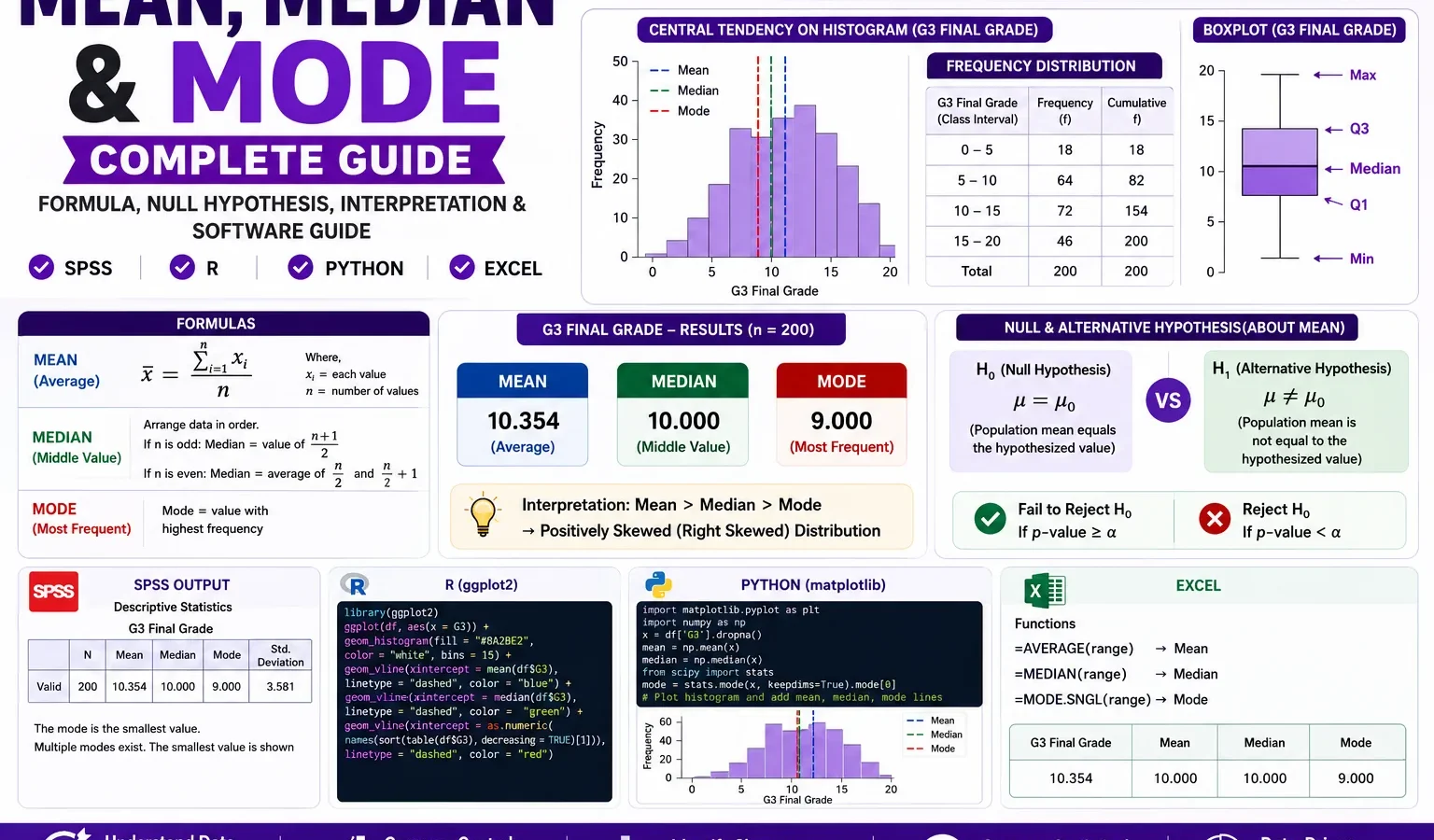
Central Tendency, Distribution Shape and Descriptive Hypothesis Decision
Mean, median and mode are the three most common measures of central tendency. They tell where the center of a variable is located, but they do it in different ways. This guide explains the meaning, formula, null hypothesis framing, interpretation, SPSS output, R charts, Python charts and Excel workflow using G3 final grade from the student-por.csv dataset.
Quick Answer: Mean, Median and Mode Result for G3
The main variable analyzed was G3 final grade. The verified SPSS, Python and R outputs show N = 649, mean = 11.91, median = 12.00 and mode = 11. The mean and median are very close, so the center of G3 is around 12 grade points. The mode is 11, meaning score 11 was the most frequent G3 score in the dataset.
Descriptive hypothesis decision: Mean, median and mode are descriptive statistics, not a formal inferential test by themselves. However, for SEO and reporting clarity, a descriptive hypothesis can be framed. The null hypothesis says the three central tendency measures are close enough to describe one common center, or H0: mean ≈ median ≈ mode. The alternative hypothesis says the center is not well described by one common value, or H1: mean, median and mode differ enough to suggest strong skewness or outlier influence. For G3, the mean and median are almost identical, while the mode is only one grade point lower. Therefore, we fail to reject the descriptive null hypothesis for the central location. The center is around 12, but the result must be qualified because SPSS also reports skewness = -0.913, showing low-score influence.
Final report sentence: Central tendency was examined for G3 final grade using 649 valid cases. The mean was 11.91, the median was 12.00 and the mode was 11. The mean and median were very close, suggesting a central location around 12. The mode showed that 11 was the most frequent score. The descriptive null hypothesis that the central tendency measures identify a common center was not rejected, although the negative skewness value and low-score outliers indicate that the distribution is not perfectly balanced.
Important note: Do not use only the mean when a distribution has skewness or outliers. For G3, the mean and median are close, but the histogram and boxplot show low-end values such as 0 and 1. That is why this post reads mean, median and mode together with histogram interpretation, box plot interpretation, frequency distribution and descriptive statistics.
Table of Contents
- What Are Mean, Median and Mode?
- Mean, Median and Mode Formula
- Null and Alternative Hypothesis for Mean, Median and Mode
- Dataset and Clean SPSS-Ready Files Used
- Verified SPSS, R and Python Results
- Python Charts and Interpretation
- R Validation Charts
- How to Calculate Mean, Median and Mode in Python, R, SPSS and Excel
- How to Report Mean, Median and Mode
- Common Mistakes
- Download SPSS Output
- FAQs
What Are Mean, Median and Mode?
Mean is the arithmetic average. It is calculated by adding all values and dividing by the number of observations. Median is the middle value after sorting the data from smallest to largest. Mode is the most frequently occurring value. These three statistics are called measures of central tendency because they describe the center of a dataset.
In a perfectly balanced distribution, the mean, median and mode are often close to each other. When the distribution is skewed or contains outliers, the three measures may separate. The mean is sensitive to extreme values, the median is more resistant to outliers, and the mode shows the most common observed value. That is why students should learn mean median and mode together rather than memorizing each one separately.
In the G3 final-grade example, the mean = 11.91, median = 12.00 and mode = 11. This means the average final grade is about 12, the middle student also has a score around 12, and the most common single score is 11. The three values tell a consistent story of a central grade range around 11 to 12, but the low-score tail means we should still review spread, skewness and the frequency distribution.
Practical meaning: Mean gives the overall average, median gives the middle score, and mode gives the most repeated score. When all three are close, the center is easier to summarize. When they differ strongly, the distribution may be skewed or affected by outliers.
Mean, Median and Mode Formula
Mean Formula
Mean = Σx / nIn this formula, Σx means the sum of all values and n means the number of observations. For G3, the SPSS output reports a mean of 11.91, meaning the average final grade is just under 12.
Median Formula
If n is odd: Median = value at position (n + 1) / 2
If n is even: Median = average of the two middle values
The median is found after arranging the values in order. For G3, the median is 12.00. This means half of the valid observations are at or below the middle position and half are at or above the middle position.
Mode Formula
Mode = value with the highest frequencyThe mode is the most repeated value. In the G3 frequency table, score 11 appears 104 times, or 16.0% of valid cases. Therefore, the mode is 11.
| Measure | G3 value | What it tells us | Best use |
|---|---|---|---|
| Mean | 11.91 | The arithmetic average final grade. | Best when the distribution has no extreme outliers or when the average is required. |
| Median | 12.00 | The middle final grade. | Best when the distribution is skewed or has outliers. |
| Mode | 11 | The most common final grade. | Best when the most frequent category or score matters. |
Null and Alternative Hypothesis for Mean, Median and Mode
Mean, median and mode are usually descriptive statistics. They do not automatically produce a p-value like a one-sample z test or a t test. Still, a hypothesis-style statement is useful when we are using central tendency to judge whether a distribution has one clear center or whether skewness/outliers make the center harder to summarize.
| Hypothesis | Statement | Meaning for G3 final grade |
|---|---|---|
| Null hypothesis | H0: mean ≈ median ≈ mode | The three central tendency measures are close enough to describe a common center. |
| Alternative hypothesis | H1: mean, median and mode are meaningfully different | The center is not described well by one value because skewness, repeated values or outliers affect the distribution. |
| Practical decision rule | Compare mean, median, mode, skewness, histogram and boxplot. | Close values support the null hypothesis; large gaps and clear tail problems support the alternative hypothesis. |
For G3, the mean is 11.91, median is 12.00 and mode is 11. The mean-median gap is only about 0.09, which is very small. The mode is one grade point lower than the median, but that is not unusual for an integer grade variable. Therefore, the descriptive decision is to fail to reject the null hypothesis that G3 has a common central location around 12.
Hypothesis decision: Fail to reject the descriptive null hypothesis for central tendency alignment. The G3 distribution has a center around 11 to 12. However, because skewness is -0.913 and the boxplot shows low-score outliers, the report should not say the distribution is perfectly symmetric. The correct interpretation is that the central tendency values are close, but the distribution has a low-score tail.
Reporting caution: This is a descriptive hypothesis framing, not a formal inferential test. To test a population mean against a specific value, use a one-sample t test, one-sample z test or confidence interval. To test distribution normality, use visual and formal checks such as the Q-Q plot normality check, Kolmogorov-Smirnov test, Lilliefors test or DAgostino Pearson test.
Dataset and Clean SPSS-Ready Files Used
This example uses the student-por.csv student performance dataset. The main outcome variable is G3 final grade. Additional numeric variables were also checked so that the post can show how mean and median behave across variables with different shapes, including G1, G2, age, absences, studytime and failures.
SPSS workflow rule: The SPSS output was generated from a clean SPSS-ready dataset. This is important because central tendency statistics depend on correctly imported numeric variables. If a numeric column is imported as text, SPSS may not calculate the mean, median and mode correctly.
| Item | Value or file | Explanation |
|---|---|---|
| Main dataset | student-por.csv | Student performance dataset used for the worked example. |
| SPSS output | Mean-Median-Mode-SPSS-Output.pdf | Verification file for frequencies, central tendency, descriptives, histograms and boxplots. |
| Main variable | G3 final grade | Main outcome used to explain mean, median and mode. |
| Valid N | 649 | All G3 cases were valid in the SPSS output. |
| Hypothesis focus | Central tendency alignment | Checks whether mean, median and mode describe one common center. |
| Software workflow | Python, R, SPSS and Excel | Python and R produced charts; SPSS produced official output; Excel formulas are shown for manual calculation. |
External dataset source: UCI Machine Learning Repository: Student Performance dataset.
Verified SPSS, R and Python Results
The SPSS output, Python charts and R charts agree on the main G3 central tendency result. The G3 final grade has mean = 11.91, median = 12.00 and mode = 11. The frequency table shows that score 11 is the most common G3 score, while the histogram and boxplot show that most values are concentrated around 10 to 15 with a small number of very low values.
Main G3 Central Tendency Result
| Statistic | G3 value | Interpretation |
|---|---|---|
| Valid N | 649 | The analysis used 649 valid G3 scores. |
| Mean | 11.91 | The average final grade is about 12. |
| Median | 12.00 | The middle final grade is 12. |
| Mode | 11 | The most frequent final grade is 11. |
| Standard deviation | 3.231 | Individual final grades vary by about 3.23 points around the mean. |
| Variance | 10.437 | The squared spread of G3 scores. |
| Minimum and maximum | 0 and 19 | The observed scores cover the full range from very low to high grades. |
| Interquartile range | 4 | The middle 50% of G3 values are spread over about four grade points. |
| Skewness | -0.913 | The low-score tail pulls the distribution to the left. |
| Kurtosis | 2.712 | The distribution has heavier tails or sharper concentration than normal. |
Hypothesis Result for Central Tendency Alignment
| Component | Result | Decision |
|---|---|---|
| Null hypothesis | H0: mean ≈ median ≈ mode | Assumes G3 has one practical center. |
| Alternative hypothesis | H1: central tendency values differ meaningfully | Assumes skewness or outliers make one center misleading. |
| Mean vs median | 11.91 vs 12.00 | Very close; supports a common center around 12. |
| Mode vs median | 11 vs 12 | Only one grade point apart; acceptable for integer grade data. |
| Skewness qualification | -0.913 | Shows low-score tail influence, so the center should be reported with distribution shape. |
| Final decision | Fail to reject H0 descriptively | G3 has a practical central location around 11 to 12, but with low-end outliers. |
Central Tendency Across Numeric Variables
| Variable | N | Mean | Median | Mode | SD | Skewness | Interpretation |
|---|---|---|---|---|---|---|---|
| G3 final grade | 649 | 11.91 | 12.00 | 11 | 3.231 | -0.913 | Mean and median are close; mode is one point lower; low-score tail exists. |
| G2 second period grade | 649 | 11.57 | 11.00 | 11 | 2.914 | -0.360 | Center is around 11 to 12 with mild left skew. |
| G1 first period grade | 649 | 11.40 | 11.00 | 10 | 2.745 | -0.003 | Nearly symmetric by skewness, with mean and median close. |
| Student age | 649 | 16.74 | 17.00 | 17 | 1.218 | 0.417 | Most students are around 16 to 17 years old. |
| School absences | 649 | 3.66 | 2.00 | 0 | 4.641 | 2.021 | Mean is much higher than median and mode, showing strong right skew and high-absence outliers. |
| Weekly study time | 649 | 1.93 | 2.00 | 2 | 0.830 | 0.700 | Most students are in study time category 2. |
| Past class failures | 649 | 0.22 | 0.00 | 0 | 0.593 | 3.093 | Most students have zero failures, with a small high-failure tail. |
G3 Frequency Table Summary
| G3 score | Frequency | Percent | Interpretation |
|---|---|---|---|
| 10 | 97 | 14.9% | One of the most common lower-central scores. |
| 11 | 104 | 16.0% | The modal value; this is the most frequent final grade. |
| 12 | 72 | 11.1% | Median value is 12, showing the central position. |
| 13 | 82 | 12.6% | Another common central/high-central score. |
| 0 | 15 | 2.3% | Low-score tail value that affects the mean and skewness. |
| 19 | 2 | 0.3% | Highest observed grade, but rare. |
Python Charts and Interpretation
1. Mean, Median and Mode for G3
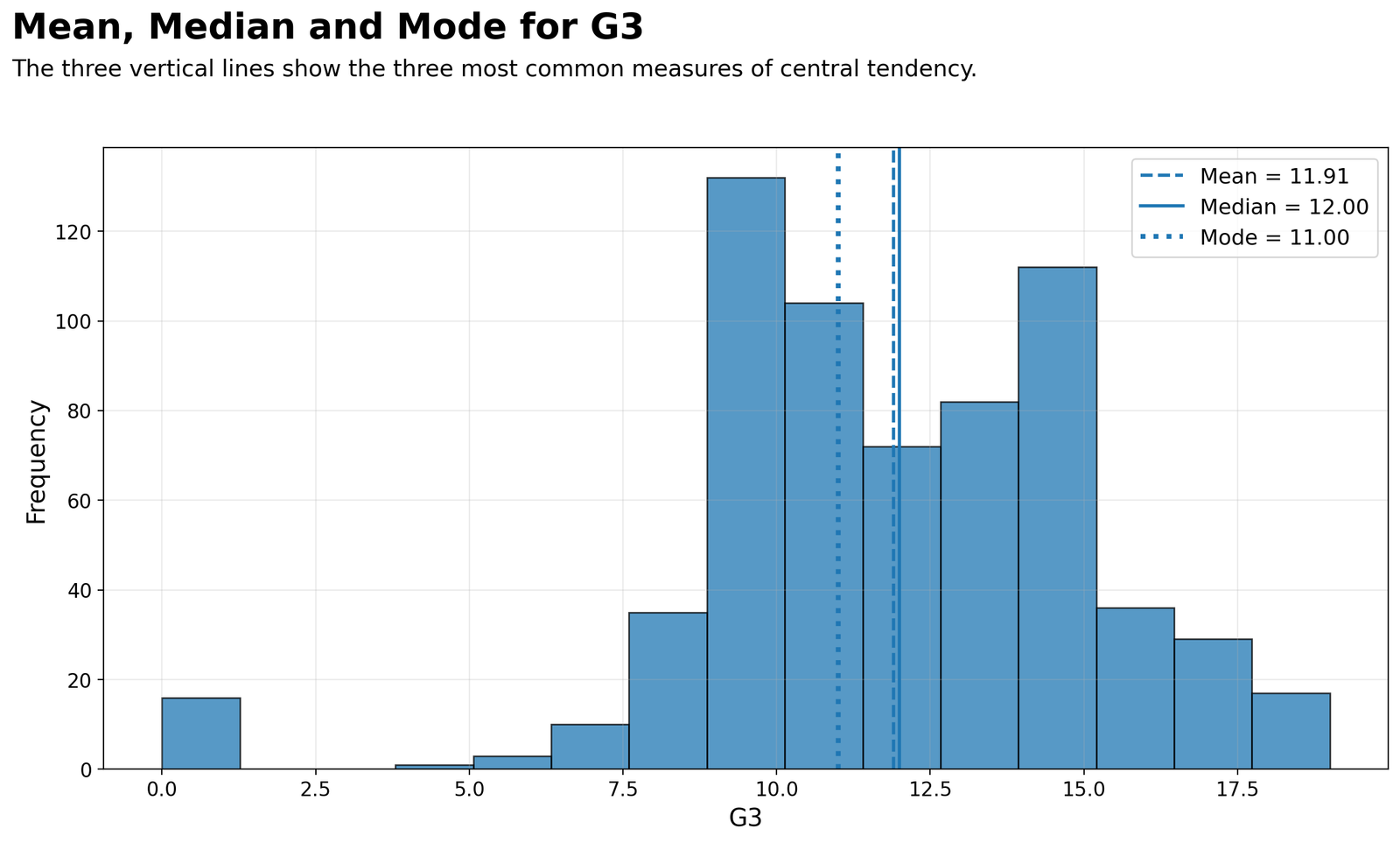
This histogram places the three central tendency measures directly on the G3 distribution. The dashed mean line is at about 11.91, the solid median line is at 12.00, and the dotted mode line is at 11.00. The bars show that most students scored between about 10 and 15, while a smaller number of students scored very low values such as 0 or 1. The mean and median lines almost overlap, which supports the descriptive null hypothesis that G3 has a common center around 12. The mode line is slightly to the left because score 11 is the most repeated exact score. This does not contradict the mean or median; it simply tells us that the single most frequent grade is 11 even though the overall center is around 12. The low-score values on the left side explain why the mean is slightly below the median and why SPSS reports negative skewness. Therefore, the chart supports a clear central-tendency conclusion while also reminding the reader that outliers and skewness should be discussed.
2. Central Tendency Comparison for G3
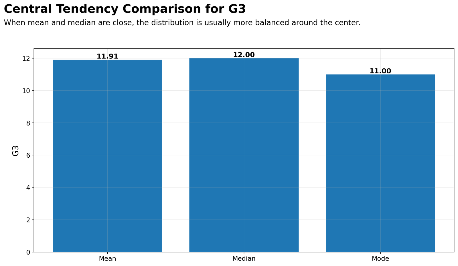
This bar chart separates the three central tendency values so they can be compared quickly. The mean bar is 11.91, the median bar is 12.00, and the mode bar is 11.00. The visual difference between mean and median is very small, which indicates that the average and the middle position give almost the same central answer. The mode is lower by one point because 11 has the highest frequency. In a discrete grade variable, the mode often differs slightly from the mean and median because it depends on one exact value rather than the full distribution. For hypothesis wording, this chart supports failing to reject the descriptive null hypothesis that the main center is consistent. The practical conclusion is that G3 is centered near 12, with 11 as the most common observed grade.
3. Mean vs Median Across Numeric Variables
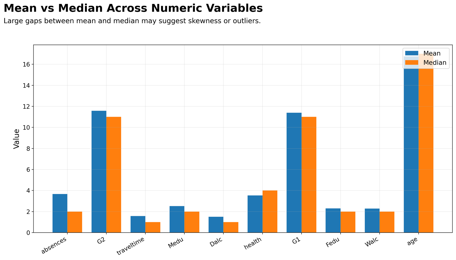
This chart compares mean and median for several numeric variables. Large gaps between the two measures suggest skewness, outliers or a bounded scale. For G3, the mean and median are very close, which supports a stable central interpretation. For G2 and G1, the mean and median are also close, suggesting that grade variables have reasonably similar central locations. The biggest contrast appears for absences, where the mean is about 3.66 and the median is 2. This large gap means absences are right-skewed: many students have low absences, but some students have high absence counts that pull the mean upward. The chart also shows why the median is often more informative for skewed count variables. For age, mean and median are close because most students are around 16 to 17. Overall, this chart teaches that mean and median should be read together. When they agree, the center is easy to summarize. When they separate, the analyst should check skewness, outliers, a histogram or a boxplot.
4. Boxplots for Central Tendency and Spread
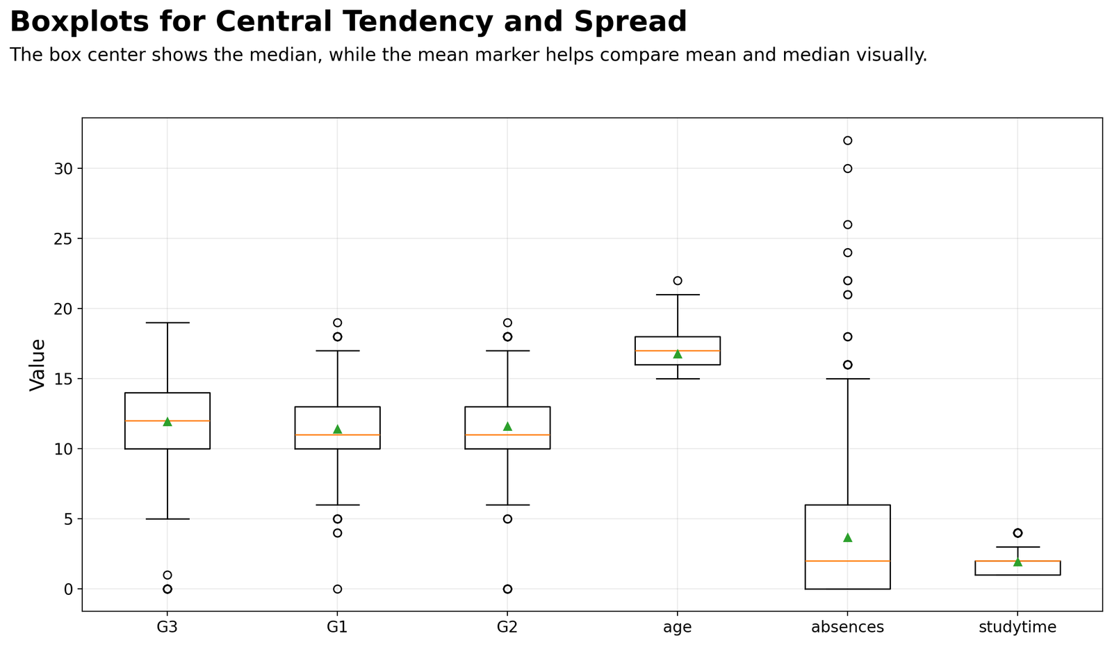
The boxplot chart explains why mean, median and mode should not be interpreted without spread. Each box shows the middle 50% of values, the line inside the box shows the median, and the marker shows the mean. For G3, the median is around 12, the box covers a moderate grade range, and several low outliers appear near 0 and 1. These low outliers explain the negative skewness and why the mean is slightly below the median. For G1 and G2, the boxes are similar but slightly lower, showing earlier grade periods with centers around 11. For age, the box is narrow because most students are in a small age range, with a few older values. For absences, the box is close to the lower end, but many high outliers extend upward, confirming strong right skew. For studytime, values are concentrated in low categories. This chart supports the conclusion that G3 has a useful central value around 12, but it also shows why central tendency must be accompanied by spread and outlier interpretation.
5. Frequency Distribution of G3
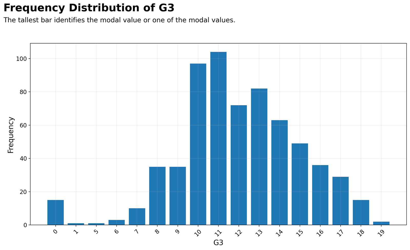
This frequency distribution shows the exact count for each G3 score. The tallest bar occurs at G3 = 11, which is why the mode is 11. The next very common values are around 10, 13, 12 and 14, showing that the central grade region is dense. The distribution also includes 15 students with G3 = 0 and only 2 students with G3 = 19. These rare edge values are important because they affect the mean and shape of the distribution. The mode is especially useful here because it identifies the most common exact score, while the median identifies the middle position and the mean uses every score. The chart supports the final interpretation that the typical G3 score is around 11 to 12, with 11 being the most frequent single value.
R Validation Charts
The R charts reproduce the same central tendency interpretation using a separate software workflow. This is useful because it confirms that the result is not limited to Python or SPSS. The R charts support the same conclusion: G3 has mean ≈ 11.91, median = 12 and mode = 11.
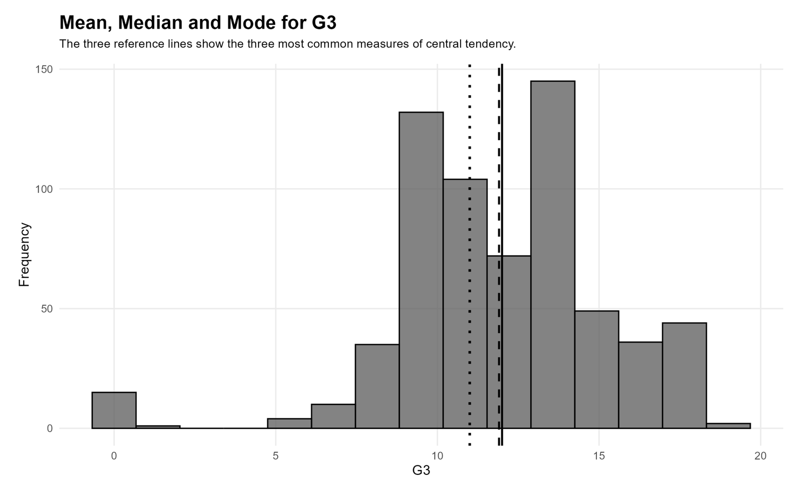
The R histogram validates the same pattern seen in Python. The mean and median reference lines are close to each other around 12, while the mode line is slightly lower at 11. Most observations are grouped in the central grade range, but a small low-score tail remains visible. This confirms the descriptive hypothesis decision: the central tendency values are close enough to describe a common center, but distribution shape still needs a short qualification.
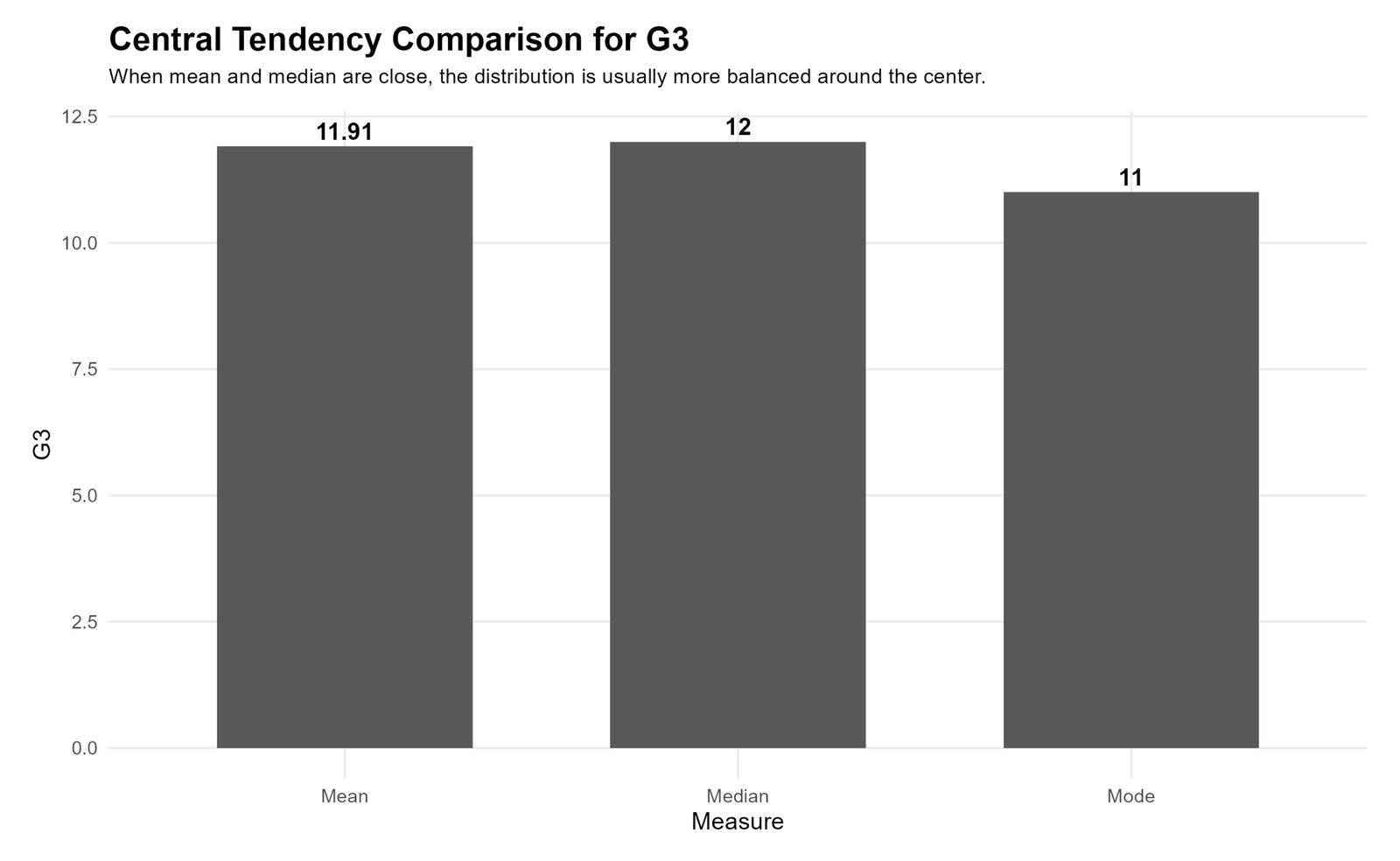
The R bar chart confirms the values mean = 11.91, median = 12 and mode = 11. The main teaching point is that the mean and median are almost identical, so the central location is stable. The mode is still useful because it identifies the most common exact grade, not the arithmetic center. In a final report, this chart can be used as a simple visual summary of the three central tendency measures.
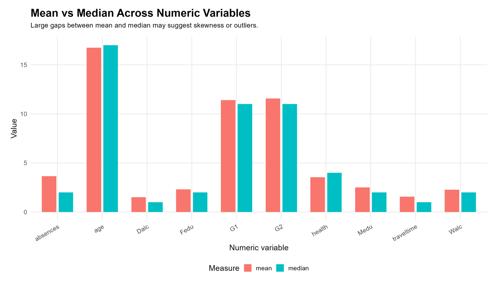
The R mean-versus-median chart confirms that G3, G1, G2 and age have relatively close mean and median values, while absences shows a much larger gap. This is exactly what the SPSS statistics show: absences has strong positive skewness, while G3 has a central mean-median alignment with a separate low-score tail. This chart is important because it prevents overgeneralization. A dataset can contain some variables with stable centers and other variables with skewed centers.
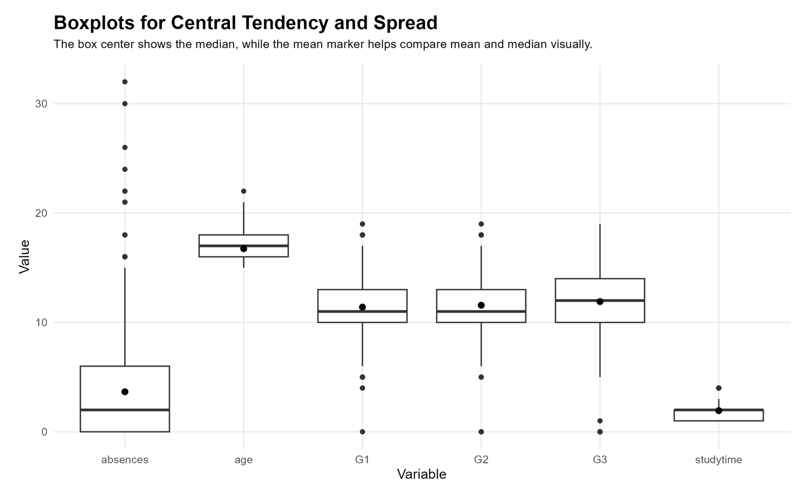
The R boxplot chart validates the spread and outlier interpretation. G3 has a central box around the middle grade range and a few very low outliers. Absences has a low median and many high outliers, which explains why its mean is much higher than its median. The chart shows that central tendency must be interpreted with distribution spread. Mean, median and mode answer “where is the center,” while boxplots answer “how spread out and unusual are the values around that center.”
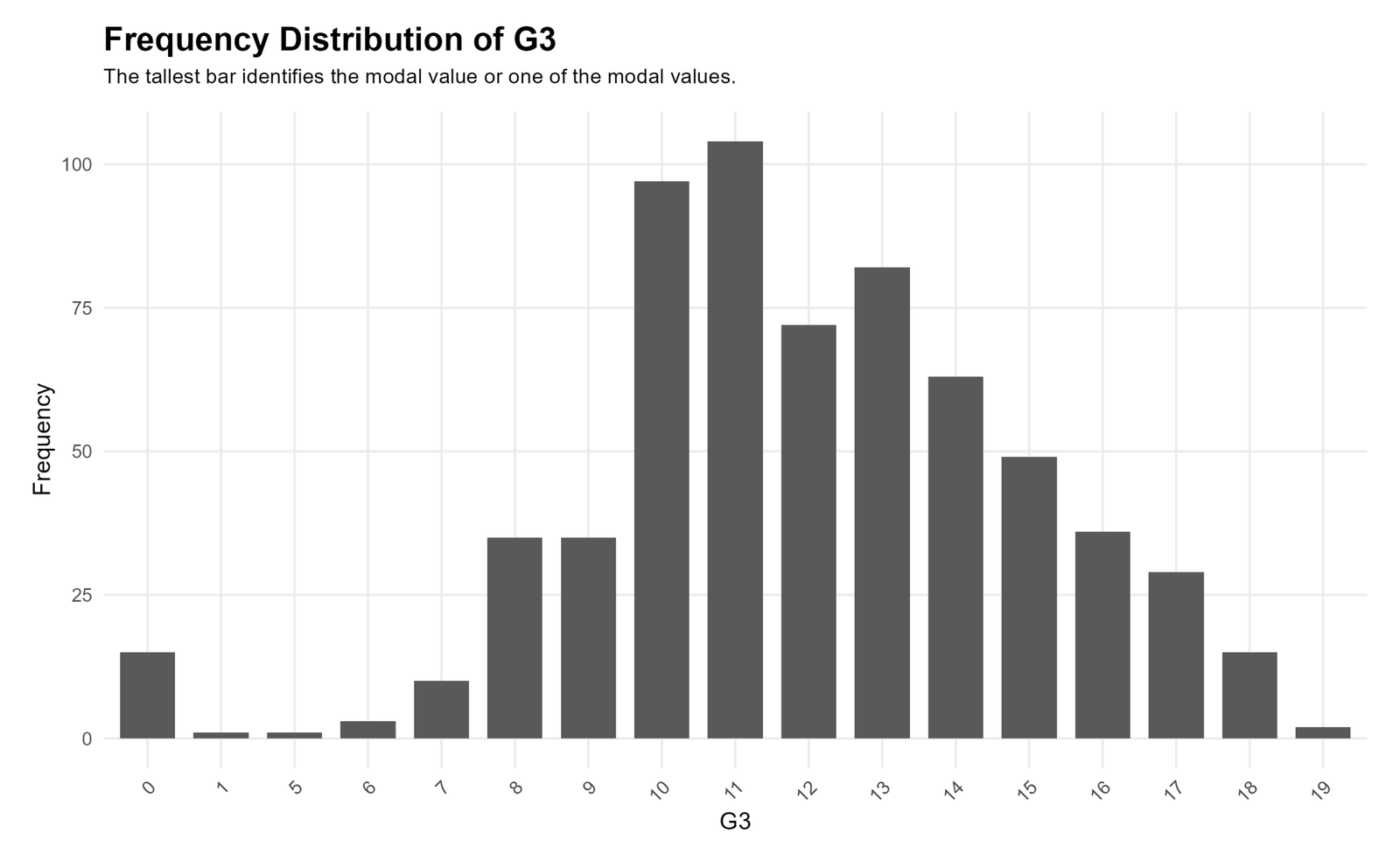
The R frequency distribution confirms that the modal value of G3 is 11. The tallest bar marks the most common score, while neighboring bars around 10 to 14 show the dense central grade region. This chart is the clearest visual support for the mode because the mode is defined by frequency, not by arithmetic calculation. It also supports the interpretation that the most typical exact score is 11, even though the overall center is around 12.
How to Calculate Mean, Median and Mode in Python, R, SPSS and Excel
Mean, Median and Mode in Python
Python can calculate mean, median, mode, frequency counts, skewness and kurtosis using pandas and scipy.
import pandas as pd
from scipy import stats

df = pd.read_csv("spss_ready_data.csv")
g3 = pd.to_numeric(df["G3"], errors="coerce").dropna()

n = g3.count()
mean_g3 = g3.mean()
median_g3 = g3.median()
mode_g3 = g3.mode().iloc[0]
sd_g3 = g3.std(ddof=1)
skew_g3 = stats.skew(g3, bias=False)
kurt_g3 = stats.kurtosis(g3, fisher=True, bias=False)

print("Null hypothesis: mean, median and mode are close enough to describe one common center.")
print("Alternative hypothesis: mean, median and mode differ enough to suggest skewness or outlier influence.")
print("N:", n)
print("Mean:", round(mean_g3, 2))
print("Median:", round(median_g3, 2))
print("Mode:", mode_g3)
print("SD:", round(sd_g3, 3))
print("Skewness:", round(skew_g3, 3))
print("Excess kurtosis:", round(kurt_g3, 3))

freq = g3.value_counts().sort_index()
print(freq)
Mean, Median and Mode in R
R calculates mean and median directly. The mode can be calculated with a small custom function because base R uses the word “mode” differently.
student <- read.csv("spss_ready_data.csv")
g3 <- na.omit(as.numeric(student$G3))

get_mode <- function(x) {
  ux <- unique(x)
  ux[which.max(tabulate(match(x, ux)))]
}

n <- length(g3)
mean_g3 <- mean(g3)
median_g3 <- median(g3)
mode_g3 <- get_mode(g3)
sd_g3 <- sd(g3)

cat("Null hypothesis: mean, median and mode are close enough to describe one common center.\n")
cat("Alternative hypothesis: central tendency values differ enough to suggest skewness or outlier influence.\n")
cat("N:", n, "\n")
cat("Mean:", round(mean_g3, 2), "\n")
cat("Median:", round(median_g3, 2), "\n")
cat("Mode:", mode_g3, "\n")
cat("SD:", round(sd_g3, 3), "\n")

print(table(g3))
Mean, Median and Mode in SPSS
SPSS can calculate mean, median and mode through the FREQUENCIES command. The syntax below also exports the SPSS output to PDF.
* Mean Median and Mode Analysis in SPSS.
* Descriptive hypothesis:
* H0: mean, median and mode are close enough to describe one common center.
* H1: central tendency measures differ enough to suggest skewness or outlier influence.

SET UNICODE=ON.
SET DECIMAL=DOT.
SET PRINTBACK=OFF.
SET MPRINT=OFF.

GET DATA
 /TYPE=TXT
 /FILE="D:\DATA ANALYSIS\A Basic Descriptive Statistics Guides\Mean Median and Mode\SPSS_Output\clean_data\spss_ready_data.csv"
 /ENCODING='UTF8'
 /DELCASE=LINE
 /DELIMITERS=","
 /QUALIFIER='"'
 /ARRANGEMENT=DELIMITED
 /FIRSTCASE=2
 /IMPORTCASE=ALL.

DATASET NAME StudentData WINDOW=FRONT.

TITLE "Mean Median and Mode Analysis".

FREQUENCIES VARIABLES=G3 G2 G1 age absences studytime failures
 /STATISTICS=MEAN MEDIAN MODE STDDEV VARIANCE SKEWNESS SESKEW KURTOSIS SEKURT RANGE MINIMUM MAXIMUM
 /ORDER=ANALYSIS.

EXAMINE VARIABLES=G3 G2 G1 absences
 /PLOT BOXPLOT HISTOGRAM
 /STATISTICS DESCRIPTIVES
 /CINTERVAL 95
 /MISSING LISTWISE
 /NOTOTAL.

EXAMINE VARIABLES=G3 BY school
 /STATISTICS DESCRIPTIVES
 /CINTERVAL 95
 /MISSING LISTWISE
 /NOTOTAL.

EXAMINE VARIABLES=G3 BY sex
 /STATISTICS DESCRIPTIVES
 /CINTERVAL 95
 /MISSING LISTWISE
 /NOTOTAL.

OUTPUT EXPORT
 /CONTENTS EXPORT=VISIBLE
 /PDF DOCUMENTFILE="D:\DATA ANALYSIS\A Basic Descriptive Statistics Guides\Mean Median and Mode\SPSS_Output\Mean-Median-Mode-SPSS-Output.pdf".
Mean, Median and Mode in Excel
Excel has direct formulas for mean, median and mode. The formulas below assume the G3 values are in cells B2:B650.
| Excel task | Example formula | Purpose |
|---|---|---|
| Sample size | =COUNT(B2:B650) | Counts valid G3 scores. |
| Mean | =AVERAGE(B2:B650) | Calculates the arithmetic average. |
| Median | =MEDIAN(B2:B650) | Finds the middle score. |
| Mode | =MODE.SNGL(B2:B650) | Finds the most frequent single score. |
| Standard deviation | =STDEV.S(B2:B650) | Measures spread around the mean. |
| Skewness | =SKEW(B2:B650) | Checks whether the distribution is pulled left or right. |
| Kurtosis | =KURT(B2:B650) | Checks tail weight using excess kurtosis. |
| Frequency of score 11 | =COUNTIF(B2:B650,11) | Confirms how often the modal value appears. |
How to Report Mean, Median and Mode
A strong central tendency report should include the sample size, mean, median, mode, standard deviation, range, skewness and a short visual interpretation. Do not report the mean alone when the distribution has outliers or skewness. For G3, the mean and median agree closely, but the mode and frequency distribution add important detail.
APA-style report: Central tendency was examined for G3 final grade using 649 valid observations. The mean was 11.91, the median was 12.00 and the mode was 11. The standard deviation was 3.231, with scores ranging from 0 to 19. The descriptive null hypothesis that the central tendency measures identify a common center was not rejected because the mean and median were nearly identical and the mode was only one point lower. However, skewness was -0.913, showing that low-score outliers influenced the distribution.
Plain-language report: The typical G3 final grade was around 12. The average score was 11.91, the middle score was 12, and the most common score was 11. Most students were clustered around the middle grade range, but a few very low scores pulled the distribution slightly to the left.
If the goal is to compare groups or test a formal mean difference, use the correct inferential test instead of only mean, median and mode. For example, compare assumptions with Levene test, Brown-Forsythe test or Cochran C test. For repeated-measures assumptions, see Mauchly’s test of sphericity and Greenhouse-Geisser correction. For model diagnostics, see Ramsey RESET test and Goldfeld-Quandt test.
Common Mistakes
1. Reporting only the mean
The mean is useful, but it can be affected by outliers. In this G3 example, the mean and median are close, but the low-score tail still matters. Always check the median, mode and distribution shape.
2. Thinking the mode is always the best “typical” value
The mode is the most frequent value, not necessarily the best overall center. For G3, the mode is 11, but the median is 12 and the mean is 11.91. The typical grade is better described as around 11 to 12.
3. Ignoring skewness
Mean and median can look close even when outliers exist. SPSS reports G3 skewness as -0.913, so the low-score tail should be mentioned.
4. Forgetting that mode can be multimodal
Some datasets have more than one mode. If two or more values are tied for the highest frequency, the distribution is multimodal. In this G3 output, score 11 is the single modal value.
5. Using mean for ordinal categories without caution
Variables such as studytime, health and famrel are ordered categories. Their means can be useful for summaries, but medians and frequency distributions are often easier to interpret.
6. Treating descriptive hypotheses as formal p-value tests
The null and alternative hypothesis in this post are descriptive framing tools. They help explain central tendency alignment. A formal hypothesis test requires a specific inferential method and a test statistic.
Download SPSS Output and Verification Files
The SPSS output PDF verifies the frequency tables, mean, median, mode, standard deviation, skewness, kurtosis, histograms, boxplots and group descriptives used in this guide.
External References for Mean, Median and Mode
This post uses verified Python, R and SPSS outputs together with standard statistical documentation and dataset references.
FAQs About Mean, Median and Mode
What are mean, median and mode?
Mean is the arithmetic average, median is the middle value after sorting the data, and mode is the most frequently occurring value.
What is the mean formula?
The mean formula is the sum of all values divided by the number of values: mean = Σx / n.
What is the median formula?
The median is the middle value after sorting the data. If the number of values is even, the median is the average of the two middle values.
What is the mode formula?
The mode is the value with the highest frequency in the dataset.
What were the mean, median and mode for G3?
For G3 final grade, the mean was 11.91, the median was 12.00 and the mode was 11.
What is the null hypothesis for mean, median and mode?
For descriptive reporting, the null hypothesis can be framed as mean, median and mode being close enough to describe one common center.
What is the alternative hypothesis for mean, median and mode?
The alternative hypothesis is that mean, median and mode differ enough to suggest skewness, outliers or an unstable central location.
What was the hypothesis decision for G3?
The descriptive null hypothesis was not rejected because mean and median were very close and the mode was only one point lower. However, low-score outliers and negative skewness should still be mentioned.
Why is the mean slightly below the median for G3?
The mean is slightly below the median because low final grades such as 0 and 1 pull the average downward.
Why is the mode 11 for G3?
The mode is 11 because score 11 appears most often in the G3 frequency table.
When should I use the median instead of the mean?
Use the median when the distribution is skewed or contains outliers, because the median is more resistant to extreme values.
How do I calculate mean, median and mode in Excel?
Use AVERAGE for the mean, MEDIAN for the median and MODE.SNGL for the mode.

