
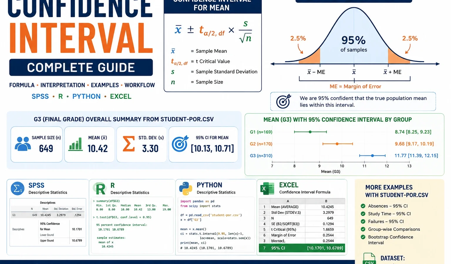
Statistical Estimation and Data Analysis
Confidence Interval is one of the most important concepts in statistics because it gives a range of reasonable values for an unknown population parameter instead of only one sample estimate. This complete guide explains how to calculate, visualize, interpret and report a 95% confidence interval using R, Python, SPSS and Excel with the student-por.csv G3 final grade example.
Quick Answer: Confidence Interval Result
A Confidence Interval was calculated for the G3 final grade variable from the student-por.csv dataset. The estimated mean final grade was 11.91. The 95% confidence interval was approximately 11.66 to 12.16. This means the sample evidence estimates the average population final grade to be around 11.91, with a reasonable 95% confidence range from 11.66 to 12.16.
Final report sentence: A 95% confidence interval was calculated for the G3 final grade mean. The sample mean was 11.91, and the 95% confidence interval ranged from 11.66 to 12.16. Therefore, the estimated population mean final grade is likely to fall within this interval under the assumptions of the confidence interval method.
Important reporting note: A confidence interval is not just a range around a graph. It is a statistical estimate of uncertainty. Do not write that there is a 95% probability that this already-calculated interval contains the true mean. A better explanation is that the confidence interval method would capture the true population mean in about 95% of repeated samples under the same conditions.
Table of Contents
- What is a Confidence Interval?
- Confidence Interval Formula and Logic
- Confidence Interval and Statistical Decision Logic
- Dataset and Variables Used
- Verified Confidence Interval Results for G3
- Chart-by-Chart Interpretation
- R Code for Confidence Interval
- Python Code for Confidence Interval
- SPSS Syntax and Interpretation
- Excel Method
- Download Output and Resources
- APA Style Reporting
- When Should You Use Confidence Intervals?
- References and Related Guides
- FAQs
What Is a Confidence Interval?
A Confidence Interval is a range of values calculated from sample data to estimate an unknown population parameter. In real data analysis, researchers usually do not observe the whole population. They collect a sample, calculate a sample statistic, and then use a confidence interval to show how precise that sample statistic is.
For example, the sample mean of G3 final grade in this analysis is approximately 11.91. This number is useful, but it is only a point estimate. A confidence interval adds uncertainty around the estimate. The 95% confidence interval for G3 is approximately 11.66 to 12.16. This range gives a more complete answer because it shows the likely location of the population mean rather than only the sample mean.
The most common confidence level is 95%, but analysts may also use 90%, 99% or another confidence level depending on the research standard. A higher confidence level usually produces a wider interval. A lower confidence level usually produces a narrower interval. This trade-off is important because more confidence requires more uncertainty space around the estimate.
Practical meaning: A confidence interval answers the question: “Based on this sample, what range of values is reasonable for the population mean?” In this example, the reasonable 95% range for the G3 mean is about 11.66 to 12.16.
Confidence intervals are widely used in education research, business analytics, medical studies, social science surveys and statistical reporting. They help readers understand whether an estimate is precise or uncertain. A narrow interval suggests a more precise estimate. A wide interval suggests more uncertainty, usually because of a smaller sample size, higher variability or higher confidence level.
For a complete statistical workflow, confidence intervals can be combined with tests such as the One-Sample Z Test, One-Tailed T Test, One-Proportion Z Test, and assumption-checking methods such as the Q-Q Plot, Kolmogorov-Smirnov Test and Lilliefors Test.
Confidence Interval Formula and Logic
The basic structure of a confidence interval is simple. A confidence interval starts with a sample estimate, then adds and subtracts a margin of error. For a mean, the sample estimate is the sample mean. The margin of error is based on the critical value and the standard error.
Confidence Interval = Point Estimate ± Margin of Error

Margin of Error = Critical Value × Standard Error

For a mean:
CI = x̄ ± t* × (s / √n)
In this formula, x̄ is the sample mean, t* is the t critical value, s is the sample standard deviation, and n is the sample size. When the population standard deviation is unknown, the t-distribution is commonly used for the confidence interval of a mean.
| Formula part | Meaning | Applied to this example |
|---|---|---|
| Point estimate | The statistic calculated from the sample | G3 mean = 11.91 |
| Standard error | Estimated sampling variability of the mean | Smaller standard error gives a narrower interval |
| Critical value | Value from t or z distribution based on confidence level | 95% confidence uses a two-sided critical value |
| Margin of error | Distance added and subtracted from the mean | About 0.25 grade points in this example |
| Lower bound | Mean minus margin of error | Approximately 11.66 |
| Upper bound | Mean plus margin of error | Approximately 12.16 |
The confidence interval is wider when the sample is more variable, the sample size is smaller, or the confidence level is higher. It is narrower when the sample size is larger, the data are less variable, or the confidence level is lower.
Confidence Interval and Statistical Decision Logic
A confidence interval is mainly an estimation tool, not only a hypothesis test. However, it can still support statistical decision-making. If a hypothesized value falls outside a confidence interval, that value may be inconsistent with the sample evidence at the corresponding confidence level. If the hypothesized value falls inside the interval, the sample evidence is not strong enough to rule it out.
| Decision idea | Meaning | Example interpretation |
|---|---|---|
| Null value inside CI | The hypothesized value is plausible | Do not reject the value using CI logic |
| Null value outside CI | The hypothesized value is not supported by the interval | Reject or question the hypothesized value |
| Narrow CI | The estimate is more precise | Sample gives a stable estimate |
| Wide CI | The estimate is less precise | More data or less variability may be needed |
In this post, the main goal is estimation. We are estimating the average G3 final grade and interpreting the uncertainty around that average. The confidence interval result is therefore more informative than the mean alone.
Dataset and Variables Used
This worked example uses the student-por.csv student performance dataset. The main variable used for the confidence interval is G3, which represents the final grade. The analysis also compares confidence intervals for G1, G2 and G3, then checks confidence intervals by school, sex, study time, past failures and absences.
| Item | Variable or value | Explanation |
|---|---|---|
| Dataset | student-por.csv | Student performance dataset used for grade-based statistical examples. |
| Main outcome | G3 | Final grade variable used for the main 95% confidence interval. |
| Comparison grade variables | G1 and G2 | Earlier grade variables used for CI comparison with G3. |
| Grouping variables | school, sex, studytime, failures | Used to compare G3 mean confidence intervals by subgroup. |
| Additional numeric variable | absences | Used to estimate confidence interval for mean absences by school. |
External dataset source: UCI Machine Learning Repository: Student Performance dataset.
Verified Confidence Interval Results for G3 Final Grade
The Confidence Interval analysis was reproduced through Python, R and SPSS output. The main conclusion is that the estimated G3 final grade mean is 11.91, and the 95% confidence interval is approximately 11.66 to 12.16. This interval is narrow enough to show a reasonably precise estimate of the mean final grade.
Main Confidence Interval Summary
| Statistic | Verified value | Interpretation |
|---|---|---|
| Variable | G3 | Final grade variable analyzed with confidence interval. |
| Mean | 11.91 | Average final grade in the sample. |
| 95% CI lower bound | 11.66 | Lower reasonable estimate for the population mean. |
| 95% CI upper bound | 12.16 | Upper reasonable estimate for the population mean. |
| Approximate margin of error | 0.25 | The mean is about 0.25 grade points away from each CI boundary. |
| Confidence level | 95% | Standard confidence level used in most academic reports. |
Interpretation of the Result
The interval 11.66 to 12.16 shows that the average G3 final grade is estimated fairly precisely. The point estimate is 11.91, but the confidence interval communicates that the population mean is not known exactly. The likely range is not extremely wide, so the sample gives a stable estimate of the final grade mean.
The bootstrap confidence interval also supports the same practical conclusion. Bootstrap resampling repeatedly draws samples from the observed data and calculates a new mean each time. When the bootstrap distribution centers near the original mean and its interval is close to the standard confidence interval, the result becomes more trustworthy for practical reporting.
Chart-by-Chart Interpretation of the Confidence Interval Analysis
This section explains each uploaded chart used in the Confidence Interval analysis. The goal is not only to display graphs, but to explain what every chart proves about the G3 final grade mean, interval width, confidence level, sample size, bootstrap uncertainty and group comparison.
Chart 1: 95% Confidence Interval for G3 Mean
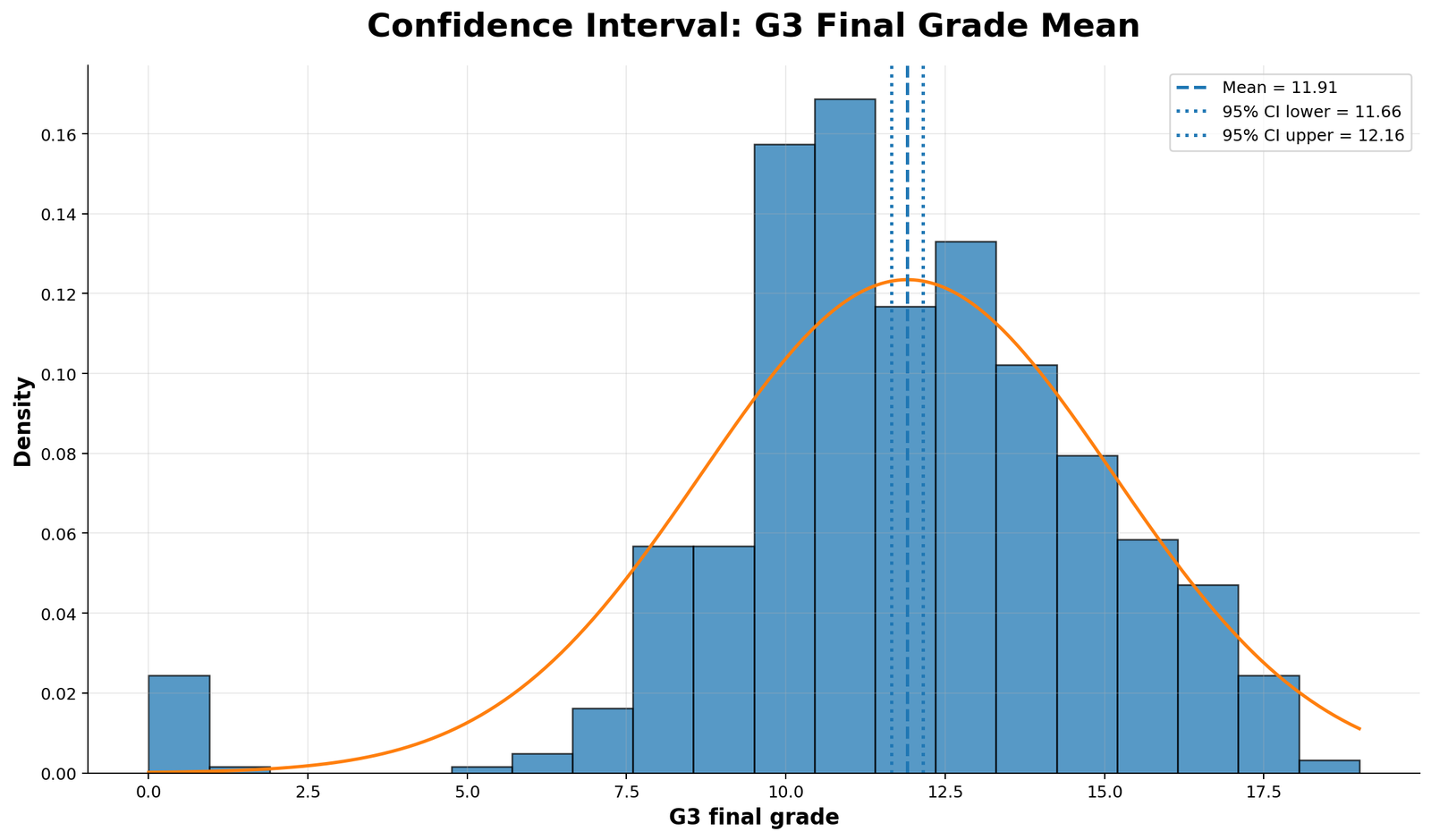
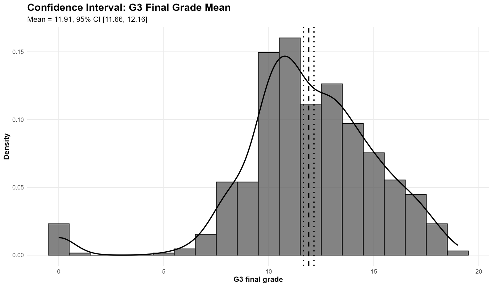
Specific interpretation: This is the main Confidence Interval chart for the G3 final grade variable. It shows the sample mean around 11.91 and the 95% confidence interval from approximately 11.66 to 12.16.
The histogram or distribution background shows how G3 scores are spread, while the vertical confidence interval markers show the uncertainty around the mean. The interval is fairly narrow, which means the estimated average final grade is reasonably precise. The mean alone tells us the center of the sample, but the interval tells us the likely range for the population mean.
Decision from Chart 1: The G3 final grade mean is estimated at 11.91, and the 95% confidence interval supports a population mean in the narrow range of 11.66 to 12.16.
Chart 2: Confidence Interval Comparison for G1, G2 and G3
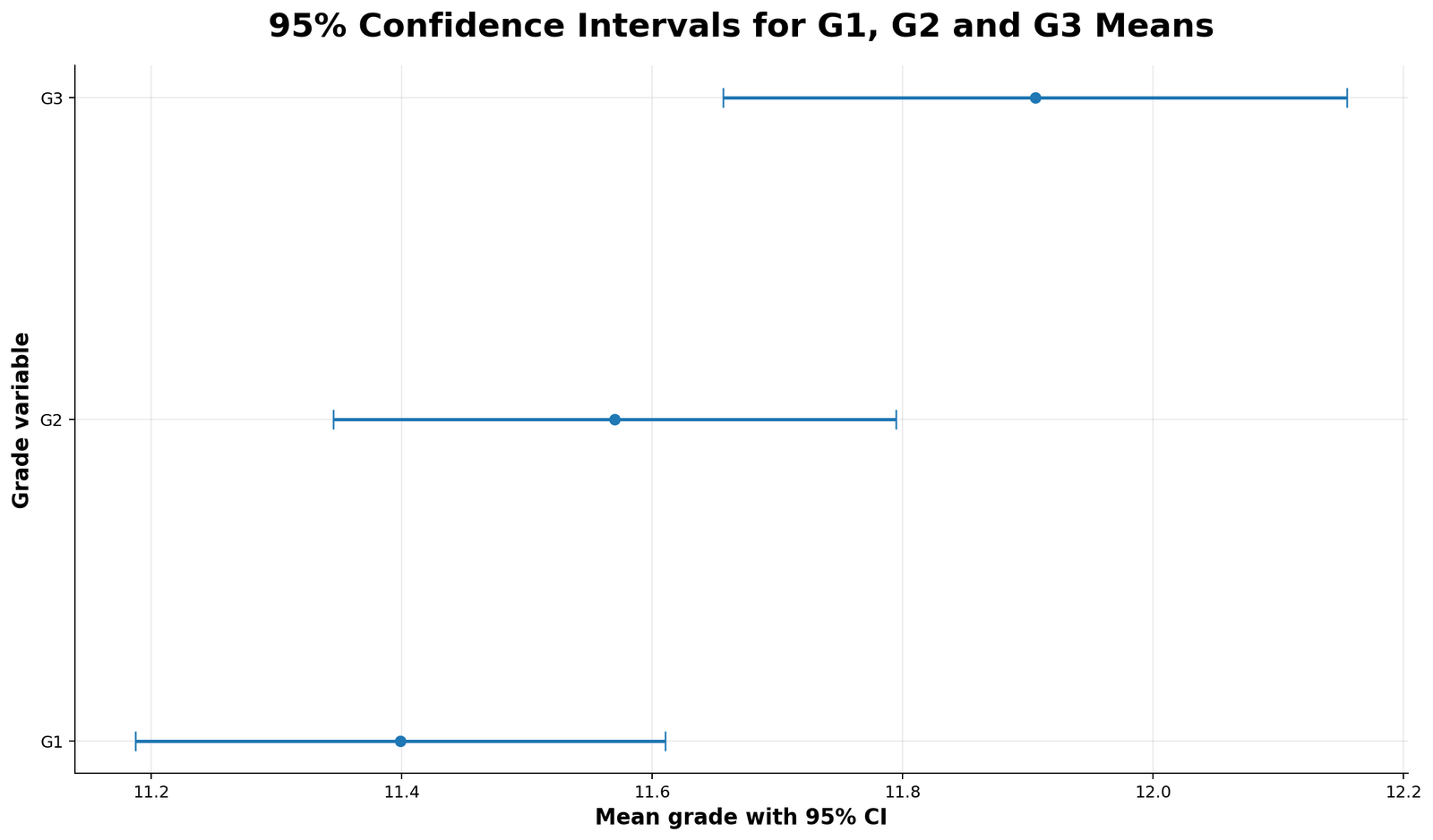
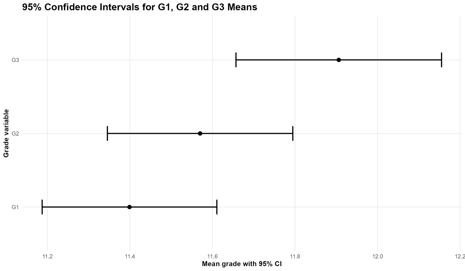
Specific interpretation: This chart compares the mean confidence intervals for G1, G2 and G3. These variables represent different grade periods. The chart shows whether the estimated average grade changes across time.
The final grade variable G3 has a mean around 11.91 and appears slightly higher than the earlier grade variables. This does not automatically prove a causal improvement, but it does show that the final grade estimate is located a little above the earlier grade estimates in this sample.
Decision from Chart 2: G3 has the highest estimated mean among G1, G2 and G3, and the confidence interval comparison makes that pattern easier to read than a simple table of means.
Chart 3: Confidence Interval Width by Confidence Level
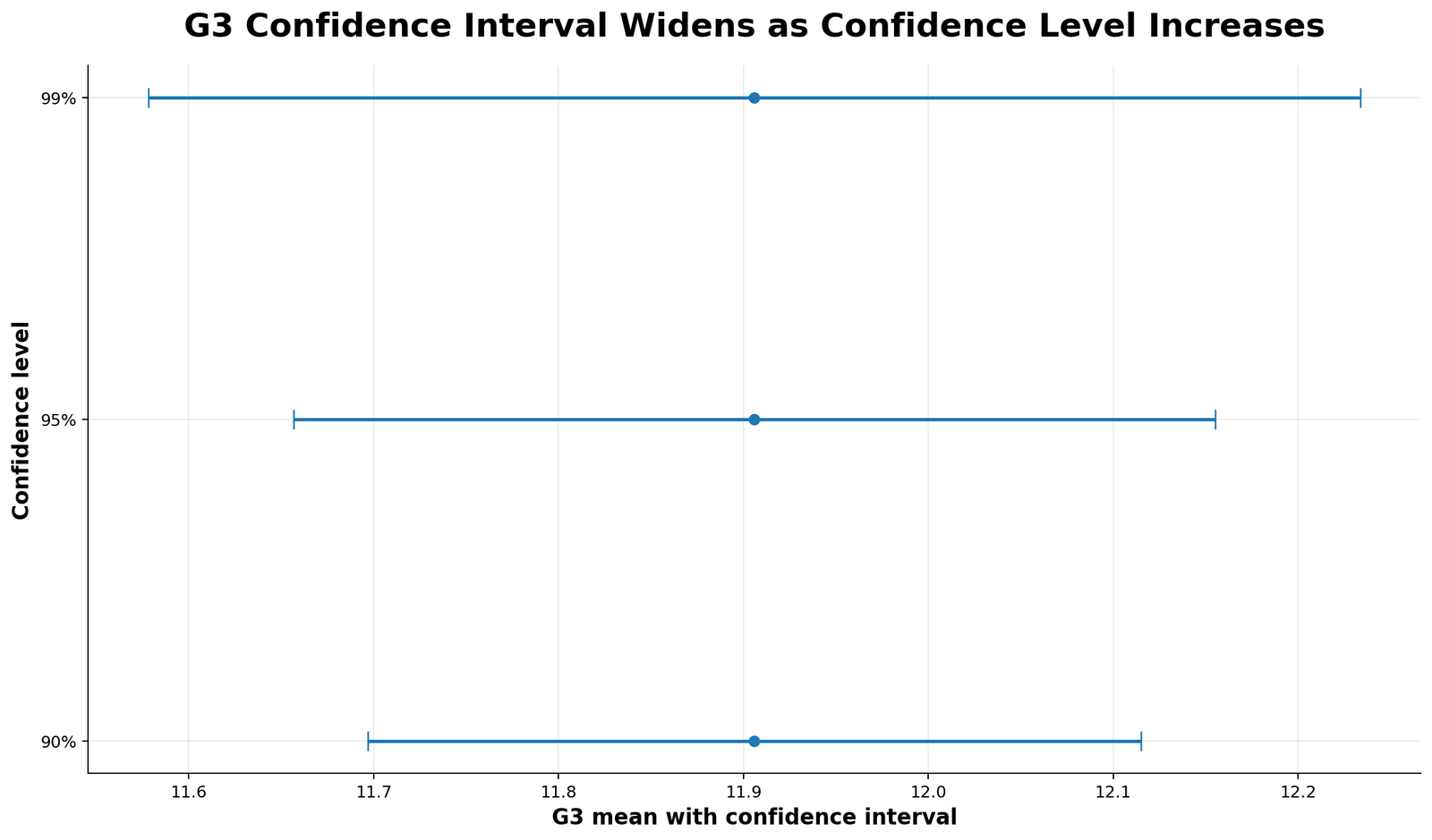
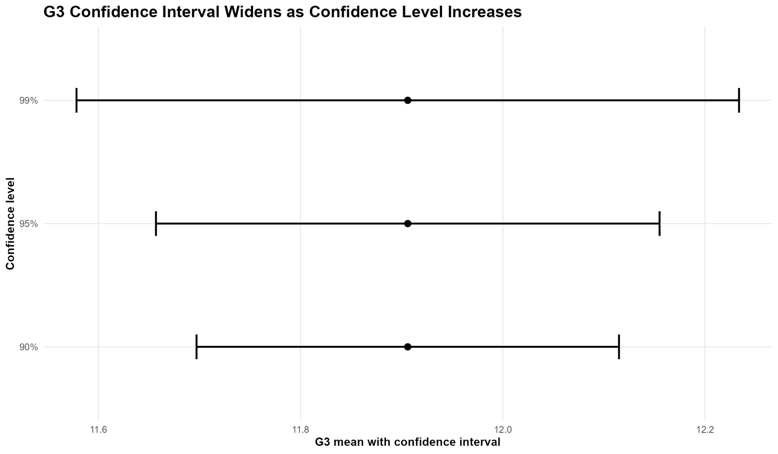
Specific interpretation: This chart shows a core rule of Confidence Interval interpretation: as the confidence level increases, the confidence interval becomes wider. A 90% confidence interval is usually narrower than a 95% confidence interval. A 99% confidence interval is usually wider than both.
This happens because a higher confidence level requires more protection against sampling error. To be more confident that the interval captures the unknown population mean, the interval must allow a larger range around the sample mean.
Decision from Chart 3: The 95% confidence interval is a balanced choice because it provides a standard level of confidence without becoming as wide as a 99% interval.
Chart 4: Confidence Interval Width by Sample Size
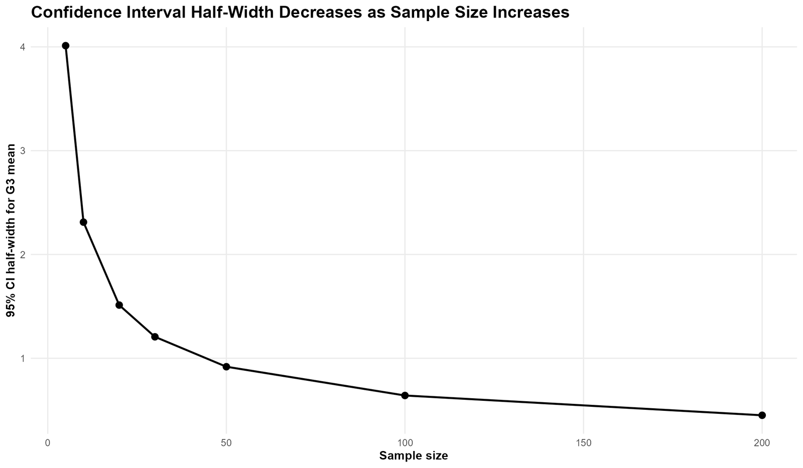
Specific interpretation: This chart explains why larger samples produce more precise estimates. As sample size increases, the standard error decreases. Because the margin of error depends on the standard error, the confidence interval becomes narrower when the sample size becomes larger.
This is one of the most important lessons for research design. If a sample is too small, the confidence interval may be wide and uncertain. If the sample is large enough, the interval becomes more stable and easier to interpret.
Decision from Chart 4: Larger samples improve precision by reducing the width of the confidence interval.
Chart 5: Bootstrap Confidence Interval for G3 Mean
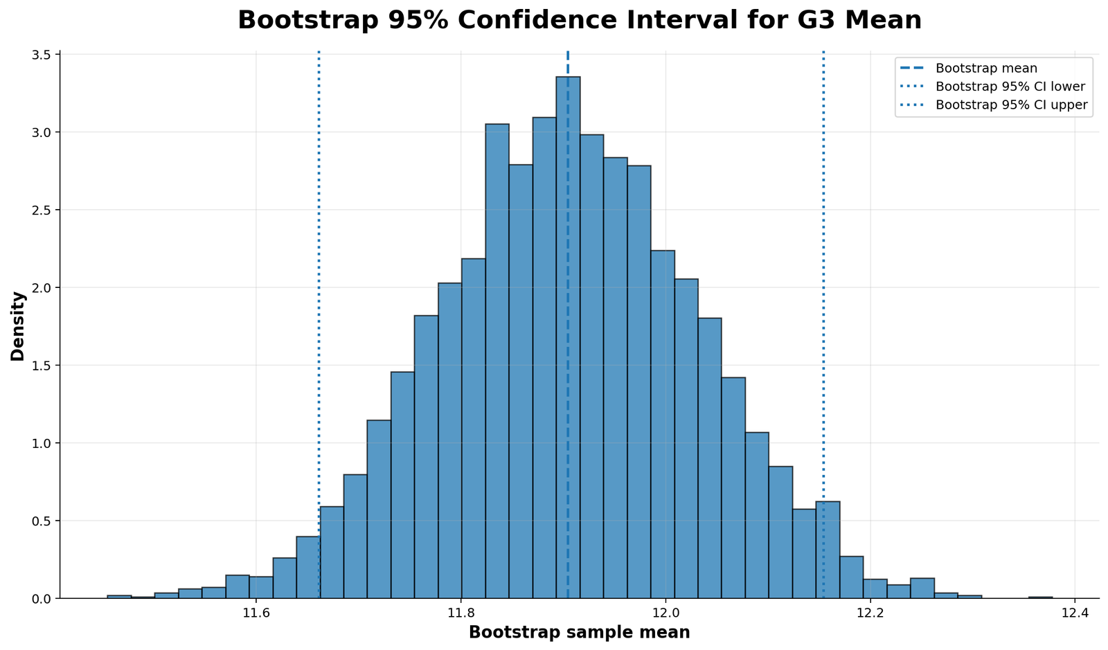
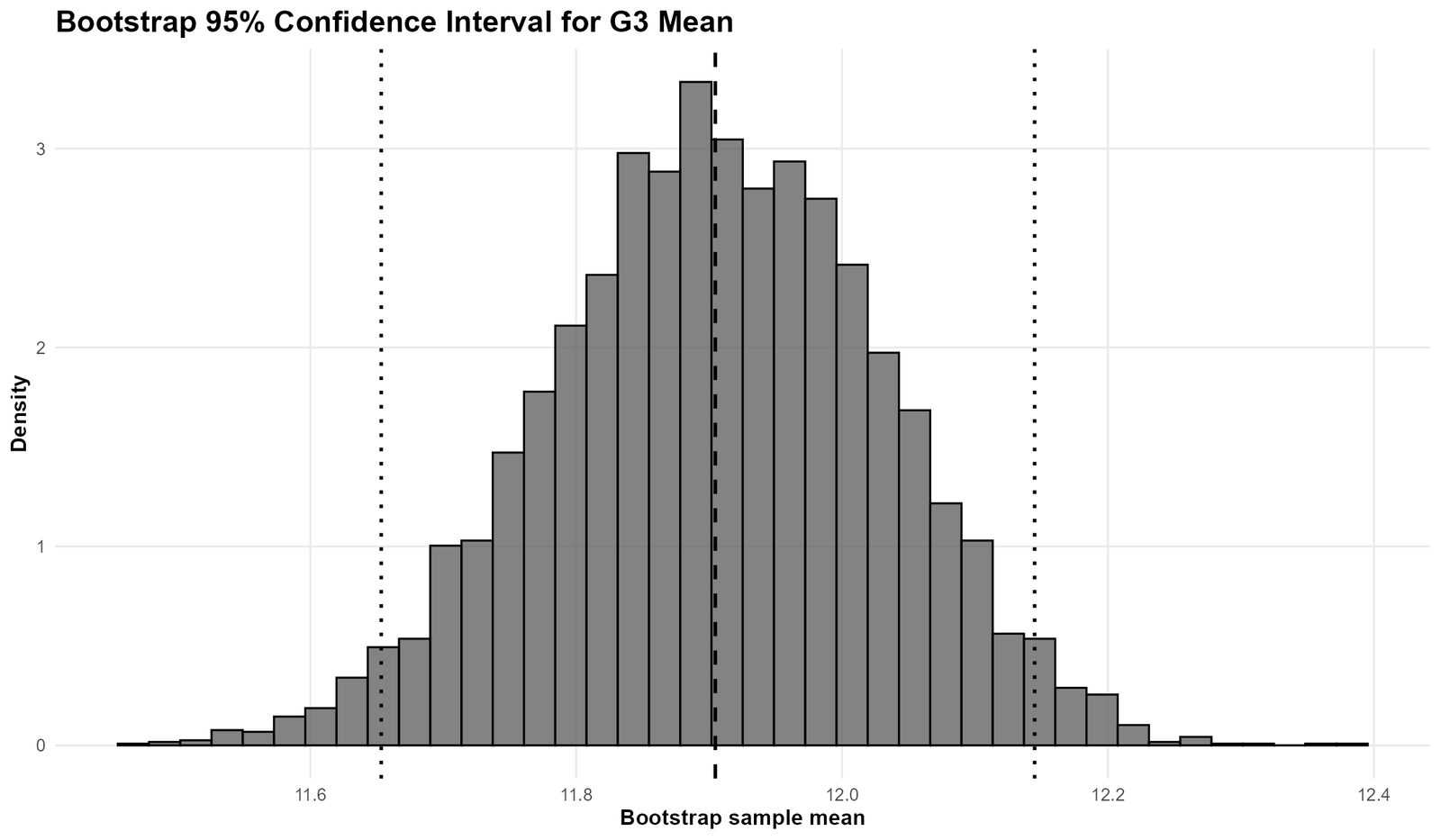
Specific interpretation: The bootstrap chart estimates the confidence interval by repeatedly resampling from the observed G3 values. Instead of relying only on a formula, the bootstrap method creates many resampled means and then uses their distribution to estimate uncertainty.
The bootstrap distribution is centered close to the original G3 mean. This supports the standard 95% confidence interval result. If the bootstrap distribution had been far away from the standard result, we would need to investigate the data or assumptions more carefully.
Decision from Chart 5: The bootstrap confidence interval supports the main conclusion that the G3 mean is estimated around 11.91 with a narrow uncertainty range.
Chart 6: G3 Confidence Interval by School
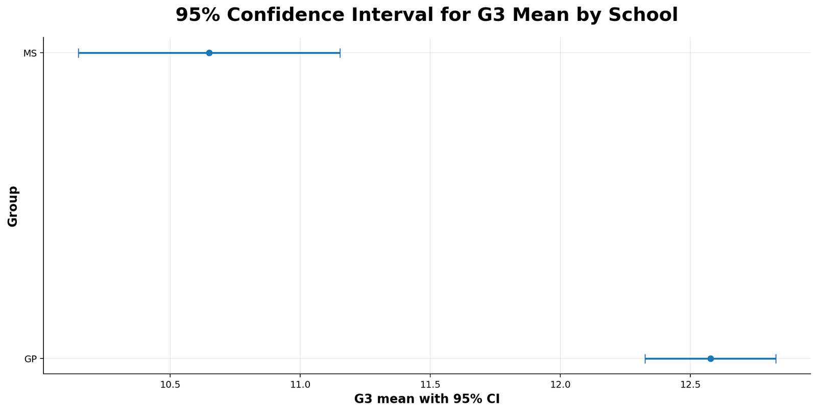
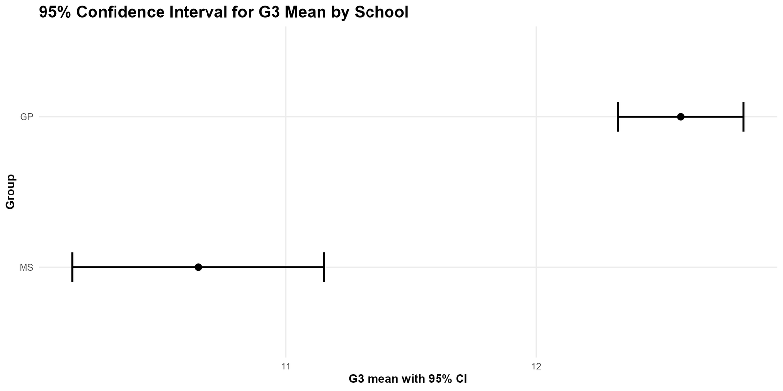
Specific interpretation: This chart compares the G3 mean confidence interval by school group. Grouped confidence intervals are useful because they show whether the mean estimate changes across categories.
In the displayed output, the GP group has a higher estimated G3 mean than the MS group. The confidence intervals help show not only which group has a higher mean, but also how precise each group estimate is. If a group has fewer observations or more variability, its confidence interval will usually be wider.
Decision from Chart 6: School group appears related to the average G3 final grade in this sample, with GP showing a higher mean estimate than MS.
Chart 7: G3 Confidence Interval by Sex
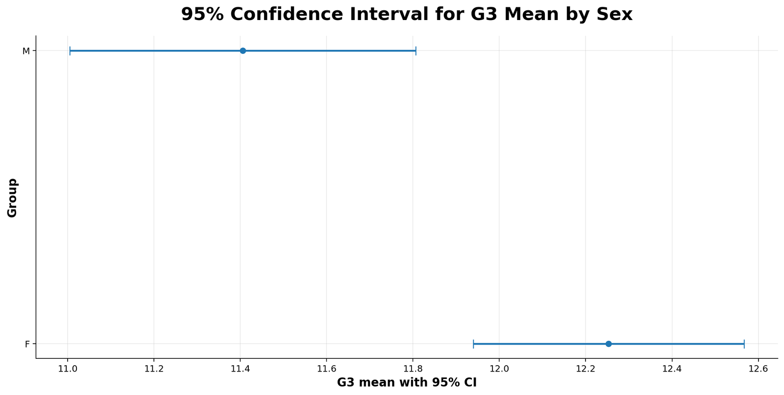
Specific interpretation: This chart compares G3 mean confidence intervals by sex group. A grouped confidence interval chart makes the comparison clearer than a table because the reader can see both the estimated mean and the uncertainty around each group mean.
The displayed chart suggests that one group has a higher estimated G3 mean than the other. The purpose of this chart is not only to rank the groups, but to show whether the group estimates are precise or uncertain. Wider intervals should be interpreted more cautiously.
Decision from Chart 7: The sex-group confidence interval chart shows a visible difference in average G3 estimates, but a formal group comparison test may be added if the research question requires hypothesis testing.
Chart 8: G3 Confidence Interval by Study Time
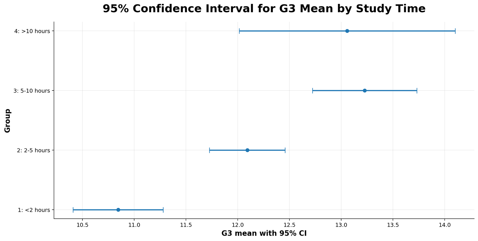
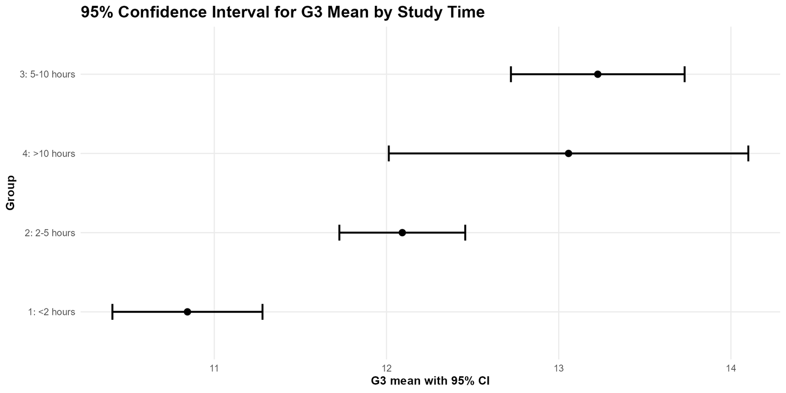
Specific interpretation: This chart compares the G3 mean across study-time categories. It is useful because it connects the confidence interval with an educational interpretation. The chart suggests that students with higher study time generally have higher mean final grades.
The confidence intervals also show precision within each study-time category. If the highest study-time category has a wider interval, this may indicate fewer observations or more variability in that category. Therefore, both mean level and interval width should be considered together.
Decision from Chart 8: Study time appears positively related to G3 final grade, and confidence intervals make the pattern more understandable.
Chart 9: G3 Confidence Interval by Past Failures
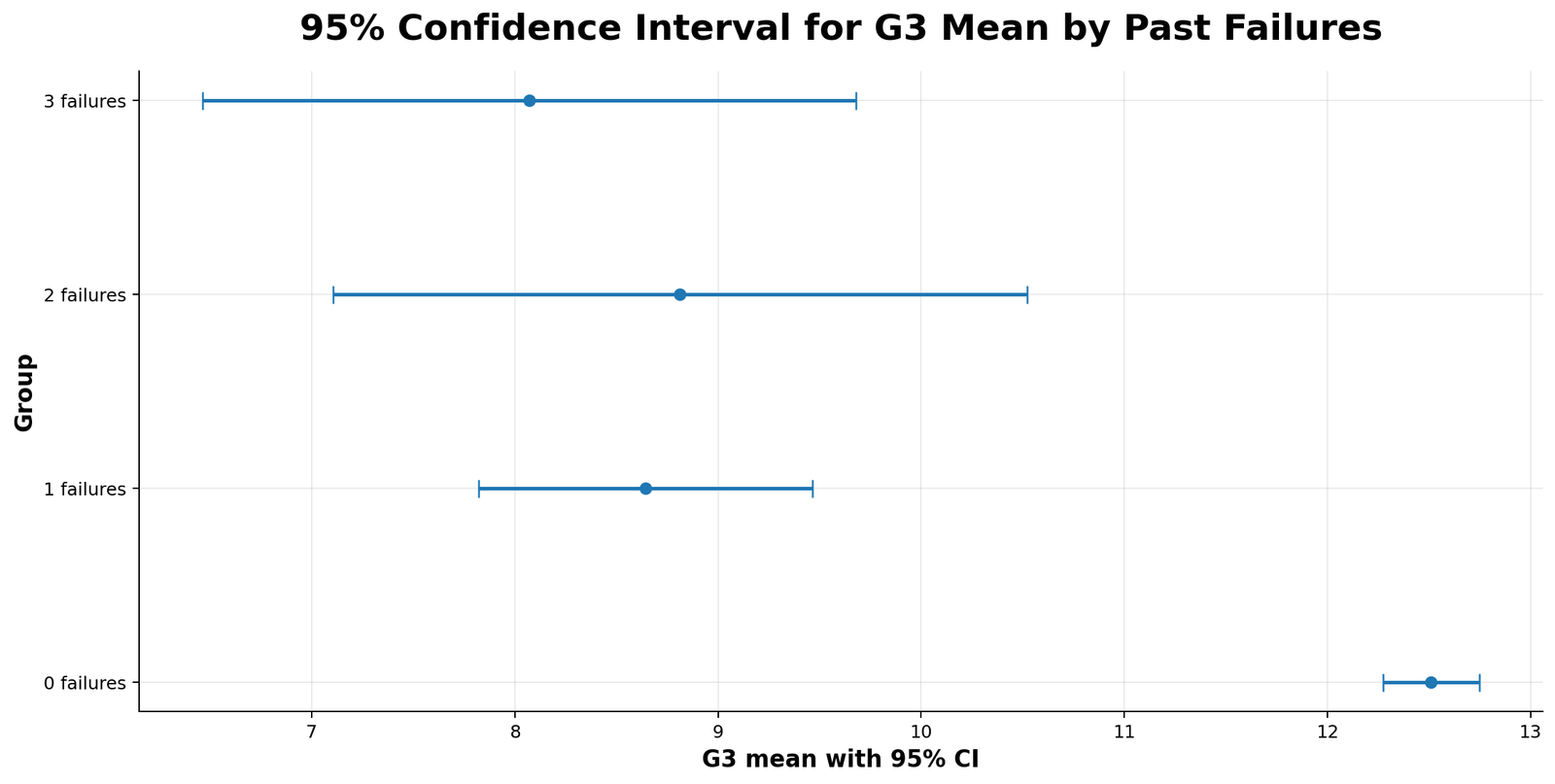
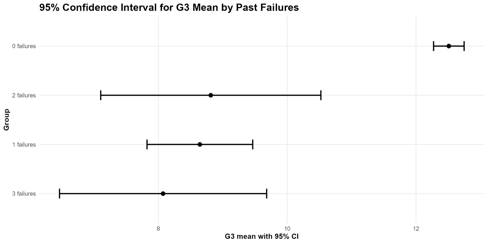
Specific interpretation: This chart shows one of the clearest group patterns in the analysis. Students with zero past failures have the highest estimated G3 mean. Students with one or more past failures show lower mean estimates, and some failure groups have wider intervals.
Past failures are strongly meaningful in educational data. A lower mean among students with more failures suggests that previous academic difficulty is associated with lower final-grade performance. However, confidence interval width must still be considered because some failure groups may contain fewer observations.
Decision from Chart 9: The zero-failures group has the strongest G3 mean estimate, while past-failure groups show lower average final grade estimates.
Chart 10: Absences Confidence Interval by School
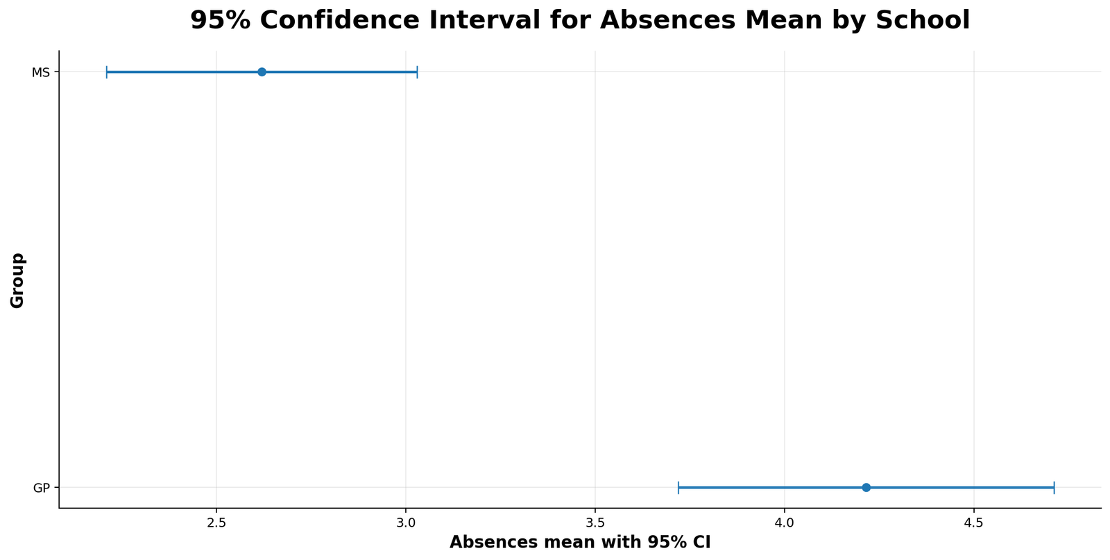
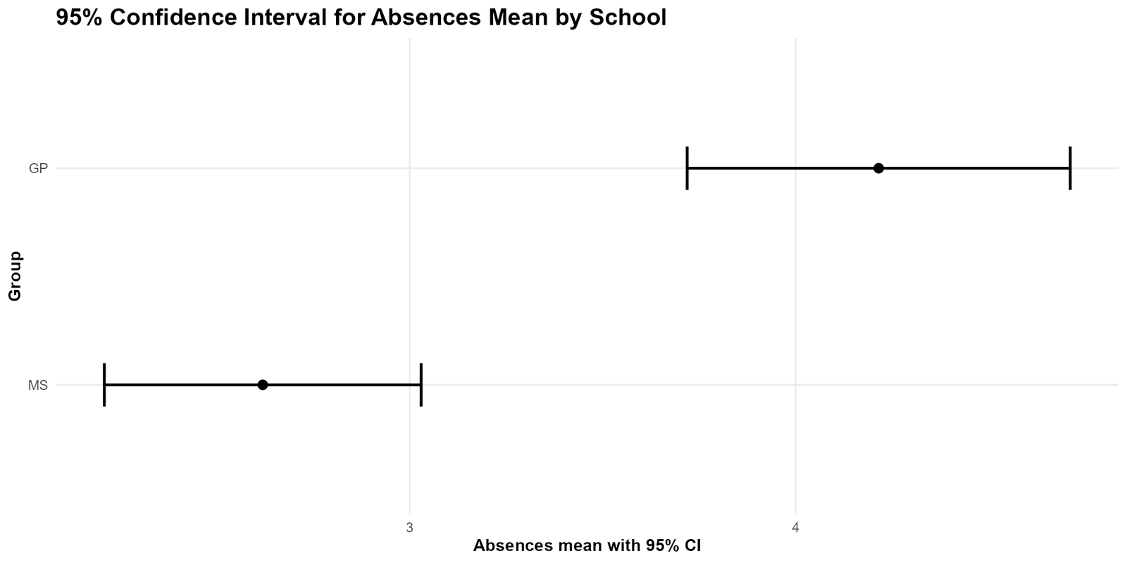
Specific interpretation: This chart applies the confidence interval method to absences rather than G3. It shows that confidence intervals are not limited to grades. They can be used for any numeric variable where a mean estimate is meaningful.
The chart compares mean absences by school group. The displayed output suggests a difference in average absences between the school groups. The confidence intervals show whether each school’s absence estimate is precise or uncertain.
Decision from Chart 10: Confidence intervals can be applied beyond the main outcome variable. Here, they help compare average absences by school group.
Final combined chart interpretation: The Confidence Interval analysis shows that the G3 final grade mean is estimated at 11.91 with a 95% confidence interval from 11.66 to 12.16. The grade comparison chart shows G3 slightly higher than G1 and G2. The confidence-level chart proves that higher confidence produces wider intervals. The sample-size chart proves that larger samples reduce interval width. The bootstrap chart supports the main estimate. Grouped charts show meaningful differences by school, sex, study time, past failures and absences.
R Code for Confidence Interval
The following R workflow can be used to calculate the 95% confidence interval for the G3 final grade mean, generate grouped confidence intervals, create charts and save results. Update the folder path before running the code.
# Confidence Interval in R
# Update this folder path before running

folder <- "D:/low kda score priority basis posts/first post/Confidence Interval"
data_file <- file.path(folder, "student-por.csv")
out_dir <- file.path(folder, "R_Output")
dir.create(out_dir, showWarnings = FALSE, recursive = TRUE)

library(readr)
library(dplyr)
library(ggplot2)

# Load data
df <- read_csv(data_file, show_col_types = FALSE)

# Clean G3
g3 <- as.numeric(df$G3)
g3 <- g3[!is.na(g3)]

# Main confidence interval
n <- length(g3)
mean_g3 <- mean(g3)
sd_g3 <- sd(g3)
se_g3 <- sd_g3 / sqrt(n)
t_crit <- qt(0.975, df = n - 1)
margin_error <- t_crit * se_g3
lower_ci <- mean_g3 - margin_error
upper_ci <- mean_g3 + margin_error

ci_summary <- data.frame(
  Variable = "G3",
  N = n,
  Mean = mean_g3,
  SD = sd_g3,
  SE = se_g3,
  Confidence_Level = "95%",
  Lower_CI = lower_ci,
  Upper_CI = upper_ci,
  Margin_Error = margin_error
)

write.csv(ci_summary, file.path(out_dir, "r_confidence_interval_g3_summary.csv"), row.names = FALSE)

# One-sample t.test also gives confidence interval
t_result <- t.test(g3, conf.level = 0.95)
capture.output(t_result, file = file.path(out_dir, "r_t_test_confidence_interval_output.txt"))

# Chart: G3 confidence interval
plot_df <- data.frame(
  variable = "G3 final grade",
  mean = mean_g3,
  lower = lower_ci,
  upper = upper_ci
)

p1 <- ggplot(plot_df, aes(x = variable, y = mean)) +
  geom_point(size = 4) +
  geom_errorbar(aes(ymin = lower, ymax = upper), width = 0.15, linewidth = 1.2) +
  labs(
    title = "95% Confidence Interval for G3 Final Grade Mean",
    subtitle = paste0("Mean = ", round(mean_g3, 2),
                      ", 95% CI [", round(lower_ci, 2), ", ", round(upper_ci, 2), "]"),
    x = "",
    y = "G3 final grade"
  ) +
  theme_minimal(base_size = 14)

ggsave(file.path(out_dir, "chart_01_r_confidence_interval_g3_mean.png"), p1, width = 10, height = 6, dpi = 200)

# Confidence intervals for G1, G2, G3
grade_ci <- df %>%
  select(G1, G2, G3) %>%
  summarise(across(everything(), list(
    n = ~sum(!is.na(.)),
    mean = ~mean(., na.rm = TRUE),
    sd = ~sd(., na.rm = TRUE)
  )))

# Function for grouped CI
make_group_ci <- function(data, group_var, outcome_var){
  data %>%
    group_by(.data[[group_var]]) %>%
    summarise(
      n = sum(!is.na(.data[[outcome_var]])),
      mean = mean(.data[[outcome_var]], na.rm = TRUE),
      sd = sd(.data[[outcome_var]], na.rm = TRUE),
      se = sd / sqrt(n),
      t_crit = qt(0.975, df = n - 1),
      lower = mean - t_crit * se,
      upper = mean + t_crit * se,
      .groups = "drop"
    )
}

school_ci <- make_group_ci(df, "school", "G3")
study_ci <- make_group_ci(df, "studytime", "G3")
failures_ci <- make_group_ci(df, "failures", "G3")
absences_school_ci <- make_group_ci(df, "school", "absences")

write.csv(school_ci, file.path(out_dir, "r_g3_ci_by_school.csv"), row.names = FALSE)
write.csv(study_ci, file.path(out_dir, "r_g3_ci_by_studytime.csv"), row.names = FALSE)
write.csv(failures_ci, file.path(out_dir, "r_g3_ci_by_failures.csv"), row.names = FALSE)
write.csv(absences_school_ci, file.path(out_dir, "r_absences_ci_by_school.csv"), row.names = FALSE)

print(ci_summary)
R interpretation: R confirms that the G3 mean is approximately 11.91 and the 95% confidence interval is approximately 11.66 to 12.16. The grouped confidence interval tables help compare G3 means across school, study time and past failures.
Python Code for Confidence Interval
The Python workflow below calculates the same confidence interval, saves clean SPSS-ready data, creates summary tables and supports chart generation. Python is especially useful because it can automate the full workflow from raw data to charts and output files.
# Confidence Interval in Python
# Update this folder path before running

import os
import numpy as np
import pandas as pd
from scipy import stats

folder = r"D:\low kda score priority basis posts\first post\Confidence Interval"
data_file = os.path.join(folder, "student-por.csv")
out_dir = os.path.join(folder, "Python_Output")
os.makedirs(out_dir, exist_ok=True)

# Load data
df = pd.read_csv(data_file)

# Clean numeric variables
for col in ["G1", "G2", "G3", "absences", "studytime", "failures"]:
    df[col] = pd.to_numeric(df[col], errors="coerce")

# Main confidence interval for G3
x = df["G3"].dropna()
n = len(x)
mean_g3 = x.mean()
sd_g3 = x.std(ddof=1)
se_g3 = sd_g3 / np.sqrt(n)

confidence = 0.95
alpha = 1 - confidence
t_crit = stats.t.ppf(1 - alpha / 2, df=n - 1)
margin_error = t_crit * se_g3
lower_ci = mean_g3 - margin_error
upper_ci = mean_g3 + margin_error

summary = pd.DataFrame({
    "Variable": ["G3"],
    "N": [n],
    "Mean": [mean_g3],
    "SD": [sd_g3],
    "SE": [se_g3],
    "Confidence_Level": ["95%"],
    "Lower_CI": [lower_ci],
    "Upper_CI": [upper_ci],
    "Margin_Error": [margin_error]
})

summary.to_csv(os.path.join(out_dir, "python_confidence_interval_g3_summary.csv"), index=False)

# Bootstrap confidence interval
rng = np.random.default_rng(123)
bootstrap_means = []

for i in range(10000):
    sample = rng.choice(x, size=len(x), replace=True)
    bootstrap_means.append(sample.mean())

boot_lower, boot_upper = np.percentile(bootstrap_means, [2.5, 97.5])

bootstrap_summary = pd.DataFrame({
    "Variable": ["G3"],
    "Bootstrap_Samples": [10000],
    "Observed_Mean": [mean_g3],
    "Bootstrap_Lower_95": [boot_lower],
    "Bootstrap_Upper_95": [boot_upper]
})

bootstrap_summary.to_csv(os.path.join(out_dir, "python_bootstrap_confidence_interval_g3.csv"), index=False)

# Grouped confidence interval function
def grouped_ci(data, group_col, outcome_col):
    rows = []
    for group, g in data.groupby(group_col):
        vals = g[outcome_col].dropna()
        n = len(vals)
        mean = vals.mean()
        sd = vals.std(ddof=1)
        se = sd / np.sqrt(n)
        t_crit = stats.t.ppf(0.975, df=n - 1)
        lower = mean - t_crit * se
        upper = mean + t_crit * se
        rows.append({
            "Group": group,
            "N": n,
            "Mean": mean,
            "SD": sd,
            "SE": se,
            "Lower_CI": lower,
            "Upper_CI": upper
        })
    return pd.DataFrame(rows)

school_ci = grouped_ci(df, "school", "G3")
sex_ci = grouped_ci(df, "sex", "G3")
study_ci = grouped_ci(df, "studytime", "G3")
failures_ci = grouped_ci(df, "failures", "G3")
absences_school_ci = grouped_ci(df, "school", "absences")

school_ci.to_csv(os.path.join(out_dir, "python_g3_ci_by_school.csv"), index=False)
sex_ci.to_csv(os.path.join(out_dir, "python_g3_ci_by_sex.csv"), index=False)
study_ci.to_csv(os.path.join(out_dir, "python_g3_ci_by_studytime.csv"), index=False)
failures_ci.to_csv(os.path.join(out_dir, "python_g3_ci_by_failures.csv"), index=False)
absences_school_ci.to_csv(os.path.join(out_dir, "python_absences_ci_by_school.csv"), index=False)

# Save SPSS-ready clean CSV
spss_cols = ["school", "sex", "studytime", "failures", "absences", "G1", "G2", "G3"]
clean_df = df[spss_cols].dropna()
clean_file = os.path.join(folder, "confidence_interval_spss_ready.csv")
clean_df.to_csv(clean_file, index=False)

print(summary)
print("Bootstrap CI:", boot_lower, boot_upper)
print("SPSS-ready file saved as:", clean_file)
Python interpretation: Python confirms the same result as R. The mean G3 final grade is about 11.91 and the 95% confidence interval is about 11.66 to 12.16. The bootstrap result supports the stability of this estimate, and the grouped confidence interval tables help explain subgroup differences.
SPSS Syntax and Interpretation for Confidence Interval
SPSS can calculate confidence intervals through the Explore procedure, One-Sample T Test, Means procedure and Descriptive Statistics output. The easiest route for a confidence interval around the mean is Analyze > Descriptive Statistics > Explore, because SPSS directly reports the confidence interval for the mean.
The uploaded SPSS confidence interval output is available below:
View Confidence Interval SPSS Output PDF
Recommended SPSS workflow: Use the clean file created by Python, named confidence_interval_spss_ready.csv. This avoids column-name errors and keeps the R, Python and SPSS results consistent.
* Confidence Interval in SPSS.
* Update the file path before running.

GET DATA
  /TYPE=TXT
  /FILE='D:\low kda score priority basis posts\first post\Confidence Interval\confidence_interval_spss_ready.csv'
  /ENCODING='UTF8'
  /DELCASE=LINE
  /DELIMITERS=","
  /QUALIFIER='"'
  /ARRANGEMENT=DELIMITED
  /FIRSTCASE=2
  /VARIABLES=
    school A10
    sex A10
    studytime F8.2
    failures F8.2
    absences F8.2
    G1 F8.2
    G2 F8.2
    G3 F8.2.
EXECUTE.

DATASET NAME ConfidenceIntervalData.

* Main 95% confidence interval for G3 mean.
EXAMINE VARIABLES=G3
  /PLOT NONE
  /STATISTICS DESCRIPTIVES
  /CINTERVAL 95
  /MISSING LISTWISE
  /NOTOTAL.

* Confidence interval comparison for G1, G2 and G3.
EXAMINE VARIABLES=G1 G2 G3
  /PLOT NONE
  /STATISTICS DESCRIPTIVES
  /CINTERVAL 95
  /MISSING LISTWISE
  /NOTOTAL.

* Confidence interval by school.
SORT CASES BY school.
SPLIT FILE LAYERED BY school.

EXAMINE VARIABLES=G3 absences
  /PLOT NONE
  /STATISTICS DESCRIPTIVES
  /CINTERVAL 95
  /MISSING LISTWISE
  /NOTOTAL.

SPLIT FILE OFF.

* Confidence interval by sex.
SORT CASES BY sex.
SPLIT FILE LAYERED BY sex.

EXAMINE VARIABLES=G3
  /PLOT NONE
  /STATISTICS DESCRIPTIVES
  /CINTERVAL 95
  /MISSING LISTWISE
  /NOTOTAL.

SPLIT FILE OFF.

* Confidence interval by study time.
SORT CASES BY studytime.
SPLIT FILE LAYERED BY studytime.

EXAMINE VARIABLES=G3
  /PLOT NONE
  /STATISTICS DESCRIPTIVES
  /CINTERVAL 95
  /MISSING LISTWISE
  /NOTOTAL.

SPLIT FILE OFF.

* Confidence interval by past failures.
SORT CASES BY failures.
SPLIT FILE LAYERED BY failures.

EXAMINE VARIABLES=G3
  /PLOT NONE
  /STATISTICS DESCRIPTIVES
  /CINTERVAL 95
  /MISSING LISTWISE
  /NOTOTAL.

SPLIT FILE OFF.
How to Read the SPSS Output
| SPSS output item | What to check | How to report it |
|---|---|---|
| Mean | Average G3 final grade | Report the sample mean before the interval. |
| Std. Error | Sampling uncertainty of the mean | Use it to understand CI width. |
| Lower Bound | Lower 95% confidence limit | Report as the beginning of the CI. |
| Upper Bound | Upper 95% confidence limit | Report as the end of the CI. |
| Grouped output | Separate CI for each group | Compare means and interval width across categories. |
Excel Method for Confidence Interval
Excel can calculate a confidence interval using built-in formulas. It is useful for students and quick assignments, although R and Python are better for automated chart generation and reproducible output.
Excel Steps
| Step | Excel action | Formula example |
|---|---|---|
| 1 | Place G3 values in one column. | Example range: A2:A650 |
| 2 | Calculate sample mean. | =AVERAGE(A2:A650) |
| 3 | Calculate sample standard deviation. | =STDEV.S(A2:A650) |
| 4 | Calculate sample size. | =COUNT(A2:A650) |
| 5 | Calculate standard error. | =STDEV.S(A2:A650)/SQRT(COUNT(A2:A650)) |
| 6 | Calculate t critical value. | =T.INV.2T(0.05,COUNT(A2:A650)-1) |
| 7 | Calculate margin of error. | =T_Critical*Standard_Error |
| 8 | Calculate lower and upper CI. | Lower = Mean - ME, Upper = Mean + ME |
Excel interpretation: If the mean is 11.91 and the margin of error is about 0.25, then the lower bound is about 11.66 and the upper bound is about 12.16. This matches the R and Python results.
Download Output and Resources
The complete SPSS output PDF for this Confidence Interval analysis is available below. It can be used to verify the confidence interval output and support the final report.
APA Style Reporting for Confidence Interval
Confidence interval reporting should include the mean, the confidence level, the lower bound, the upper bound and a clear interpretation. Do not report only the graph. The written interpretation is important for academic assignments, thesis work and professional analysis reports.
APA-style report: A 95% confidence interval was calculated for the G3 final grade mean. The sample mean was 11.91, and the 95% confidence interval ranged from 11.66 to 12.16. This indicates that the population mean final grade is estimated to fall within this interval under the assumptions of the confidence interval method.
For a shorter report, use the following version:
The mean G3 final grade was 11.91, 95% CI [11.66, 12.16]. The interval suggests that the population mean final grade is estimated to fall between 11.66 and 12.16.When Should You Use Confidence Intervals?
Use a Confidence Interval whenever you want to estimate a population value from a sample and communicate uncertainty clearly. Confidence intervals are useful for means, proportions, regression coefficients, group differences, odds ratios, risk ratios and many other statistical estimates.
| Analysis situation | What confidence interval estimates | Why it helps |
|---|---|---|
| Mean grade analysis | Average score or grade | Shows uncertainty around the sample mean. |
| Survey proportion | Percentage or proportion | Shows uncertainty around the sample percentage. |
| Group comparison | Mean by school, sex or treatment group | Shows both group mean differences and precision. |
| Regression analysis | Coefficient estimate | Shows plausible values for the effect size. |
| Bootstrap analysis | Empirical uncertainty from resampling | Supports estimation when assumptions are difficult. |
Important: A confidence interval is often more informative than a p-value because it shows the estimated range and practical size of the result. A p-value can help with decision-making, but a confidence interval helps with interpretation.
References and Related Guides
This guide uses the student-por.csv dataset and focuses on practical Confidence Interval interpretation. For deeper assumption testing and related statistical workflows, read these connected guides:
| Related guide | Why it helps |
|---|---|
| One-Sample Z Test | Connects confidence intervals with hypothesis testing for a mean. |
| One-Proportion Z Test | Useful for confidence intervals and hypothesis tests for proportions. |
| Q-Q Plot | Helps check whether normality assumptions are reasonable. |
| Kolmogorov-Smirnov Test | Formal distribution comparison and normality checking. |
| Lilliefors Test | Normality testing when mean and standard deviation are estimated. |
| Cramer von Mises Test | Distribution-based normality testing with full-sample sensitivity. |
| Brown-Forsythe Test | Useful when comparing group variability and checking assumptions. |
| Influence Diagnostics | Regression diagnostics, unusual observations and residual checks. |
FAQs About Confidence Interval
What is a Confidence Interval in simple words?
A Confidence Interval is a range around a sample estimate. It shows where the population value is likely to fall based on sample data and the selected confidence level.
What does a 95% confidence interval mean?
A 95% confidence interval means the method is designed to capture the true population parameter in about 95% of repeated samples under the same conditions. In this example, the G3 95% CI is approximately 11.66 to 12.16.
What is the Confidence Interval result for G3 final grade?
The G3 final grade mean is approximately 11.91, and the 95% confidence interval is approximately 11.66 to 12.16.
Why is the confidence interval better than only reporting the mean?
The mean gives only one value. The confidence interval gives a range and shows how precise or uncertain that mean estimate is.
Why does a 99% confidence interval become wider?
A 99% confidence interval becomes wider because it requires more confidence. To be more confident, the interval must allow a larger range around the sample estimate.
Why does sample size affect confidence interval width?
Larger sample size reduces the standard error. A smaller standard error produces a narrower confidence interval and a more precise estimate.
Can I calculate Confidence Interval in SPSS?
Yes. In SPSS, you can use Analyze > Descriptive Statistics > Explore and request the confidence interval for the mean. You can also use One-Sample T Test or syntax-based EXAMINE commands.
Can I calculate Confidence Interval in Excel?
Yes. Excel can calculate a confidence interval using AVERAGE, STDEV.S, COUNT, SQRT and T.INV.2T formulas. You calculate the mean, standard error, t critical value, margin of error, lower bound and upper bound.
What is a bootstrap confidence interval?
A bootstrap confidence interval is created by repeatedly resampling the observed data and calculating the statistic many times. The interval is then estimated from the resampled statistic distribution.
How should I report a confidence interval in APA style?
Report the mean, confidence level and interval bounds. Example: The mean G3 final grade was 11.91, 95% CI [11.66, 12.16].

