Hypothesis Test for One Binary Outcome
One Proportion Z Test is used to test whether one observed sample proportion is significantly different from a hypothesized population proportion. This guide explains the one sample proportion z test with null hypothesis, alternative hypothesis, formula, assumptions, p-value, confidence interval, SPSS image output, Python charts, R validation charts and Excel workflow using a student final exam pass/fail example where pass = G3 ≥ 10.
Google AdSense top placement reserved here
Quick Answer: One Proportion Z Test Result
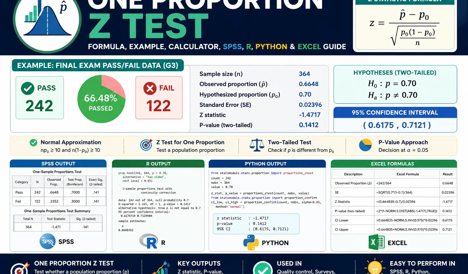
The One Proportion Z Test was performed to test whether the final exam pass proportion was different from a hypothesized value of p0 = 0.50. The binary outcome was created from the final grade variable G3. Students with G3 ≥ 10 were coded as pass, and students with G3 < 10 were coded as fail.
Out of 649 valid students, 549 passed and 100 failed. The observed sample pass proportion was p-hat = 549 / 649 = 0.8459, or about 84.6%. This observed proportion is much higher than the null hypothesis value of 0.50.
The null standard error was approximately 0.0196. The test statistic was z = 17.6248, and the two-tailed p-value was extremely small, approximately 1.59 × 10-69. In a final report, this should be written as p < .001, not as p = .000. The 95% confidence interval for the observed pass proportion was approximately [0.8181, 0.8737].
Final conclusion: Since p < .001, reject the null hypothesis. The sample provides very strong evidence that the population final exam pass proportion is significantly different from 50%. Because the observed sample proportion is 84.6%, the practical conclusion is that the pass rate is much higher than the 50% benchmark.
Important reporting note: Some software output may display a very small p-value as .000. That does not mean the p-value is exactly zero. The correct reporting style is p < .001.
Table of Contents
- What Is a One Proportion Z Test?
- When Should You Use a One Proportion Z Test?
- Null and Alternative Hypothesis
- One Proportion Z Test Formula
- Conditions and Assumptions
- Dataset and Variable Coding
- Verified Results Summary
- SPSS Image Output and Interpretation
- Python Charts and Interpretation
- R Validation Charts and Interpretation
- Overall Image Interpretation
- How to Run the Test in SPSS, Python, R and Excel
- How to Report the One Proportion Z Test
- Common Mistakes
- FAQs
What Is a One Proportion Z Test?
A One Proportion Z Test is a statistical hypothesis test used when the outcome variable has two categories and the research question is about one population proportion. The two categories are usually coded as success and failure. In this post, success means passing the final exam, and failure means not passing the final exam.
The test compares an observed sample proportion, called p-hat, with a hypothesized population proportion, called p0. If the observed difference between p-hat and p0 is large relative to its standard error, the z statistic becomes large and the p-value becomes small. A small p-value means the observed sample proportion would be unlikely if the null hypothesis were true.
For this example, the observed sample proportion is the final exam pass proportion. The null hypothesis benchmark is 0.50. The main question is: Is the population pass proportion different from 50%?
This test belongs to the broader topic of hypothesis testing. For background concepts, see Null and Alternative Hypothesis, P Value, Standard Error, Z Score and Standard Normal Distribution.
When Should You Use a One Proportion Z Test?
Use a one sample proportion z test when you have one sample, one binary outcome and one benchmark proportion. The benchmark may come from a theory, policy target, historical value, industry claim or research hypothesis.
| Situation | Use One Proportion Z Test? | Reason |
|---|---|---|
| Testing whether a final exam pass rate differs from 50% | Yes | The outcome is binary and the comparison is against one hypothesized proportion. |
| Testing whether a website conversion rate is greater than 5% | Yes | Conversion status is success/failure, and 5% is the benchmark. |
| Testing whether a survey support rate is less than 40% | Yes | Support can be coded as success, and 40% is the null value. |
| Comparing pass rates between two schools | No | That is a two-group proportion question, not a one-proportion question. |
| Testing whether the mean final grade differs from 10 | No | That uses a mean-based test, such as a One Sample Z Test or one-sample t test. |
The One Proportion Z Test is not the same as a two-proportion z test, chi-square test or logistic regression. The subgroup images by school, sex and study time are useful for descriptive context, but the main test in this post is still one overall pass proportion compared with p0 = 0.50.
Null and Alternative Hypothesis for One Proportion Z Test
The hypotheses describe what the test is checking. In this post, the null hypothesis says that the population final exam pass proportion is exactly 50%. The alternative hypothesis says that the population final exam pass proportion is different from 50%.
| Hypothesis | Symbolic form | Meaning in this example |
|---|---|---|
| Null hypothesis | H0: p = 0.50 | The population final exam pass proportion is 50%. |
| Alternative hypothesis | H1: p ≠ 0.50 | The population final exam pass proportion is not 50%. |
| Decision rule | Reject H0 if p-value < α | Using α = .05, reject H0 because p < .001. |
This is a two-tailed test because the alternative hypothesis uses “not equal to.” If the research question were specifically whether the pass proportion is greater than 50%, the alternative hypothesis would be H1: p > 0.50. If the research question were specifically whether the pass proportion is less than 50%, the alternative hypothesis would be H1: p < 0.50.
Decision in this example: The observed sample pass proportion is far above the null value. The z statistic is very large and the p-value is far below .05. Therefore, the null hypothesis is rejected.
One Proportion Z Test Formula and Calculation
The One Proportion Z Test formula is:
z = (p-hat - p0) / sqrt[p0(1 - p0) / n]

where:
p-hat = observed sample proportion
p0    = hypothesized population proportion under H0
n     = sample size
The formula standardizes the difference between the observed sample proportion and the null proportion. The denominator is the null standard error. This standard error is based on p0, not p-hat, because the hypothesis test asks what would happen if the null hypothesis were true.
| Component | Value | Explanation |
|---|---|---|
| Sample size | n = 649 | Total valid students included in the test. |
| Success count | x = 549 | Students who passed the final exam. |
| Observed proportion | p-hat = 549 / 649 = 0.8459 | Observed final exam pass proportion. |
| Null proportion | p0 = 0.50 | Hypothesized population pass proportion. |
| Null standard error | SE0 = 0.0196 | sqrt[0.50 × 0.50 / 649]. |
| Z statistic | z = 17.6248 | The observed proportion is 17.6 null standard errors above the null value. |
| Two-tailed p-value | p < .001 | The result is statistically significant. |
p-hat = 549 / 649
p-hat = 0.8459

SE0 = sqrt[0.50(1 - 0.50) / 649]
SE0 = 0.0196

z = (0.8459 - 0.50) / 0.0196
z = 17.6248
The confidence interval uses the observed proportion standard error:
SE_observed = sqrt[p-hat(1 - p-hat) / n]

95% CI = p-hat ± 1.96 × SE_observed

95% CI ≈ 0.8459 ± 1.96 × 0.0142
95% CI ≈ [0.8181, 0.8737]
The confidence interval is entirely above 0.50, which supports the same conclusion as the p-value. For a full guide to interval interpretation, see Confidence Interval and Margin of Error.
Conditions and Assumptions for One Proportion Z Test
The One Proportion Z Test uses the normal approximation to the sampling distribution of a proportion. The following conditions should be checked before trusting the z statistic and p-value.
| Condition | How to check it | This example |
|---|---|---|
| Binary outcome | Each observation must be coded into two categories. | Pass = G3 ≥ 10 and fail = G3 < 10. |
| One sample | The test should analyze one sample proportion. | The test uses one overall student sample with n = 649. |
| Independence | Each observation should represent a separate case. | Each row is treated as one independent student record. |
| Large-sample normal approximation | n × p0 and n × (1 − p0) should usually be at least 10. | 649 × .50 = 324.5 and 649 × .50 = 324.5, so the condition is satisfied. |
If the sample size were small or the expected success/failure counts were very low, an exact binomial test would be safer. In this example, the sample size is large, so the normal approximation is appropriate.
Dataset and Variable Coding
This example uses student performance data. The original final grade variable is G3. To run a one proportion z test, G3 is converted into a binary pass/fail variable.
| Item | Value | Explanation |
|---|---|---|
| Original outcome | G3 final grade | Final grade on a 0 to 20 scale. |
| Binary outcome | pass_final | New variable coded as pass or fail. |
| Success category | 1 = Pass | G3 ≥ 10. |
| Failure category | 0 = Fail | G3 < 10. |
| Sample size | 649 | Total valid cases used in the test. |
| Pass count | 549 | Number of successes. |
| Fail count | 100 | Number of failures. |
External dataset source: UCI Machine Learning Repository: Student Performance dataset.
Google AdSense middle placement reserved here
Verified SPSS, Python and R Results Summary
The SPSS image output, Python charts and R validation charts all support the same statistical conclusion. The observed pass proportion is much higher than the null value of 0.50, the z statistic is very large and the p-value is far below the .05 significance level.
| Statistic | Value | Interpretation |
|---|---|---|
| Success definition | G3 ≥ 10 | A student passed the final exam. |
| Failure definition | G3 < 10 | A student did not pass the final exam. |
| Total sample size | 649 | All valid student records. |
| Pass count | 549 | Number of successes. |
| Fail count | 100 | Number of failures. |
| Observed pass proportion | 0.8459 | About 84.6% of students passed. |
| Null proportion | 0.50 | The hypothesized benchmark. |
| Z statistic | 17.6248 | The observed proportion is extremely far above the null value. |
| Two-tailed p-value | p < .001 | Reject H0. |
| 95% confidence interval | [0.8181, 0.8737] | The estimated population pass proportion is far above 0.50. |
Main interpretation: The overall pass rate is statistically significantly different from 50%. Because the observed pass rate is 84.6%, the result indicates a much higher pass proportion than the null benchmark.
SPSS Image Output and Interpretation
The sample post used a PDF-style SPSS output explanation. In this updated version, the SPSS output is explained through individual image files. Each SPSS image below is interpreted in the same detailed style as the Python and R charts, so the reader can understand what each graph means and how it supports the final One Proportion Z Test decision.
1. SPSS Image: Pass and Fail Counts

This SPSS image shows the most important raw information for the One Proportion Z Test: the number of students who passed and the number who failed. The pass/fail variable is binary, so every student belongs to one of only two categories. The image shows 549 students in the pass category and 100 students in the fail category. This confirms that the success count is much larger than the failure count.
For the one proportion z test, the pass count is the success count x, and the total number of students is the sample size n. Therefore, this image directly supplies the values used to calculate the observed sample proportion. The observed pass proportion is 549 / 649 = 0.8459. In plain language, about 84.6% of the students passed the final exam.
The image also helps readers understand why the final result is statistically significant. If the null hypothesis were true and the population pass proportion were really 50%, the pass and fail counts would be expected to be much closer to equal. Instead, the pass count is more than five times the fail count. This visible imbalance is the first sign that the observed sample proportion is far above the null benchmark.
2. SPSS Image: Observed Proportion Compared with Null Proportion

This SPSS image compares the observed sample proportion, p-hat = 0.8459, with the null hypothesis proportion, p0 = 0.50. This comparison is the central idea of the One Proportion Z Test. The test asks whether the observed distance between these two values is large enough to reject the null hypothesis.
The gap between 0.8459 and 0.50 is approximately 0.3459, or 34.6 percentage points. This is a very large practical difference. The chart makes the difference visible before the formal z statistic is even calculated. The observed bar is far above the null benchmark line or reference value, which means the sample pass proportion is not close to the hypothesized 50% value.
Statistically, this difference is then divided by the null standard error. Because the sample size is large, the standard error is small. A large observed difference divided by a small standard error produces a very large z statistic. That is why this image leads naturally to the final decision to reject the null hypothesis.
3. SPSS Image: Confidence Interval for the Pass Proportion

This SPSS image shows the confidence interval for the estimated pass proportion. The observed pass proportion is approximately 0.8459, and the 95% confidence interval is approximately [0.8181, 0.8737]. This interval estimates the plausible range of values for the population pass proportion based on the sample data.
The confidence interval is important because it gives more information than the p-value alone. The p-value tells us whether the null hypothesis should be rejected. The confidence interval shows the likely size of the population pass proportion. In this case, even the lower bound of the interval, about 0.818, is far above the null value of 0.50.
Because the entire interval lies above 0.50, the interval supports the same conclusion as the z test. The population pass rate is not merely slightly above 50%; it appears to be substantially above 50%. This makes the result both statistically significant and practically meaningful.
4. SPSS Image: Z Statistic on the Standard Normal Curve

This SPSS image places the z statistic on the standard normal curve. The z statistic is approximately 17.6248. A z value this large is extremely far to the right of the center of the standard normal distribution. The center of the curve is zero, which represents no standardized difference from the null value. A value of 17.6 is far beyond the usual rejection boundary.
For a two-tailed test at α = .05, the usual critical values are about -1.96 and +1.96. The observed z statistic is far greater than +1.96. This means the observed sample pass proportion is far outside the range of values expected under the null hypothesis.
The visual message of this SPSS image is simple: the observed result is not close to the null value. The p-value is extremely small because almost no area remains in the tail beyond such an extreme z statistic. Therefore, the decision is to reject H0: p = 0.50.
5. SPSS Image: Pass Proportion by School

This SPSS image gives subgroup context by school. The overall One Proportion Z Test uses all students together, but this chart helps explain how the overall pass rate is distributed across school categories. The GP school group has 391 passes out of 423 students, which is approximately 92.4%. The MS school group has 158 passes out of 226 students, which is approximately 69.9%.
The chart shows that both school groups have pass proportions above 50%, but the GP group has a noticeably higher pass proportion than the MS group. This helps explain why the overall pass proportion is high. However, this image should be interpreted as descriptive context, not as the main hypothesis test. The One Proportion Z Test tests the overall pass proportion against 0.50; it does not formally test whether GP and MS differ from each other.
If the research goal were to test whether the two school pass proportions are significantly different, a two-proportion z test or a chi-square test of association would be more appropriate. For related categorical summaries, see Cross Tabulation.
6. SPSS Image: Pass Proportion by Sex

This SPSS image shows descriptive pass proportions by sex. Female students have 333 passes out of 383 students, giving a pass proportion of approximately 86.9%. Male students have 216 passes out of 266 students, giving a pass proportion of approximately 81.2%.
The chart shows that both groups have pass rates well above the 50% benchmark. The female pass proportion is slightly higher than the male pass proportion in this sample, but both groups contribute to the high overall pass proportion. This supports the broader interpretation that the overall pass rate is high across major subgroups.
Again, this image is not the formal One Proportion Z Test itself. It is a descriptive breakdown. The main test uses 549 / 649 as the overall sample proportion. A separate inferential test would be needed to claim a statistically significant difference between female and male pass proportions.
7. SPSS Image: Pass Proportion by Study Time

This SPSS image shows pass proportions across study time categories. The chart provides helpful educational context because study time is naturally related to exam performance. Students in study time category 1 have 162 passes out of 212, or about 76.4%. Category 2 has 264 passes out of 305, or about 86.6%. Category 3 has 90 passes out of 97, or about 92.8%. Category 4 has 33 passes out of 35, or about 94.3%.
The pattern is clearly increasing. Higher study time categories have higher pass proportions. This does not prove causality, because many other factors may also be related to study time and exam performance. However, it gives useful descriptive context for the overall high pass proportion.
For the One Proportion Z Test, the key point is that the overall pass proportion is high. This study time image shows that the high pass rate is not limited to a single category; it appears especially strong among students with more study time. A separate group comparison or regression model would be needed to formally test the study time pattern.
Python Charts and Interpretation
The Python charts validate the same One Proportion Z Test result using a programmatic workflow. Python is useful because it makes the calculation transparent: count successes, compute p-hat, compute the null standard error, calculate the z statistic, obtain the p-value and plot the confidence interval and subgroup summaries.
1. Python Chart: Pass and Fail Counts

The Python count chart confirms the same binary outcome used in the SPSS image output. The chart displays 549 passes and 100 failures. This verifies that the Python workflow is using the same success definition: pass = G3 ≥ 10.
This chart is important because every later statistic depends on these two counts. The sample proportion is not entered manually; it is calculated from the count of successes divided by the total number of valid cases. Therefore, the chart confirms the foundation of the test: x = 549 and n = 649.
The large difference between the pass bar and the fail bar visually explains why the observed sample proportion is far above 0.50. If the null value of 0.50 were a good description of the population, the sample would be expected to show a much more balanced pass/fail split. The Python chart shows a strong imbalance in favor of passing.
2. Python Chart: Observed Proportion versus Null Proportion

The Python observed-versus-null chart shows the central comparison in the test. The observed sample pass proportion is approximately 0.8459, while the null hypothesis value is 0.50. The visual distance between these two values is large.
This chart helps readers understand what the z statistic measures. The z statistic does not simply report that the observed value is higher; it measures how many null standard errors separate the observed proportion from the null proportion. Since the gap is about 0.3459 and the null standard error is about 0.0196, the standardized difference becomes very large.
The Python chart therefore supports the same conclusion as the SPSS image: the observed pass proportion is not close to the 50% benchmark. The statistical test then confirms that the difference is too large to treat as random sampling variation.
3. Python Chart: Confidence Interval for the Pass Proportion

The Python confidence interval chart gives the interval estimate around the observed pass proportion. The observed proportion is approximately 0.8459, and the 95% confidence interval is approximately [0.8181, 0.8737]. This means the estimated population pass proportion is likely in the low-to-high 80% range.
The interval is narrow because the sample size is large. With 649 valid cases, the sampling uncertainty around the observed proportion is relatively small. This is why the confidence interval does not stretch down near 0.50. The entire interval remains well above the null benchmark.
The Python chart is especially useful for interpretation because it shows statistical significance and practical size at the same time. The p-value tells us that the difference is significant, while the confidence interval tells us that the population pass proportion is likely much higher than 50%.
4. Python Chart: Z Statistic on the Standard Normal Curve

The Python standard normal curve chart displays the test statistic relative to the standard normal distribution. Under the null hypothesis, z values near zero are common. Values beyond about ±1.96 are already considered statistically significant for a two-tailed test at α = .05. The observed value, z = 17.6248, is far beyond that threshold.
This chart visually explains why the p-value is so small. The p-value is the tail probability of observing a z statistic as extreme as the one obtained, assuming the null hypothesis is true. Since the observed z statistic is extremely far out in the right tail, the probability is effectively tiny.
The correct interpretation is not simply that the sample pass rate is high. The correct inferential interpretation is that the sample pass rate is much higher than expected under H0: p = 0.50, and the difference is statistically significant.
5. Python Chart: Pass Proportion by School

The Python school chart validates the subgroup pattern shown in the SPSS section. The GP school has a higher pass proportion than the MS school. Specifically, GP has approximately 92.4% passing students, while MS has approximately 69.9% passing students.
This chart is useful because it shows that the overall pass proportion is a combined result from two different school groups. GP contributes a very high pass proportion, while MS is lower but still above the 50% benchmark. The overall pass rate of 84.6% is therefore not mysterious; it reflects strong pass rates across the dataset, especially in the larger GP group.
However, this Python chart should not be interpreted as a formal school comparison test. It is descriptive. The main One Proportion Z Test uses the overall sample proportion, not separate school-specific tests.
6. Python Chart: Pass Proportion by Sex

The Python sex chart shows that both female and male students have pass proportions above 80%. Female students have an approximate pass proportion of 86.9%, and male students have an approximate pass proportion of 81.2%.
This chart reinforces the overall interpretation. The total pass proportion is high because the pass rate is high in both sex groups. Although the female pass proportion is higher in this sample, the chart by itself does not prove a statistically significant sex difference. It is a descriptive chart that supports the broader understanding of the dataset.
In the context of the One Proportion Z Test, the main message is that the overall pass proportion remains far above 50% even when the data are viewed by sex. The Python chart therefore supports the same conclusion as the SPSS output and the main test calculation.
R Validation Charts and Interpretation
The R charts provide a second independent validation of the same result. R repeats the count, proportion, confidence interval, standard normal curve and subgroup interpretations. The value of the R section is that it confirms the same statistical story using a different software workflow.
1. R Chart: Pass and Fail Counts

The R pass/fail count chart confirms the same counts used by SPSS and Python. There are 549 passing students and 100 failing students. This confirms that the R workflow is using the same binary coding rule: G3 ≥ 10 is pass and G3 < 10 is fail.
This chart matters because the One Proportion Z Test is entirely built from the number of successes and the total sample size. The pass count gives x = 549, and the combined pass/fail count gives n = 649. The sample proportion is then calculated as x / n.
The R count chart also provides a simple visual check for data-entry or coding errors. If the pass/fail counts were different from the SPSS or Python output, the test result would need to be checked. Since the counts match, the workflows are consistent.
2. R Chart: Observed Proportion Compared with Null Proportion

The R observed-versus-null chart confirms that the observed sample pass proportion is far above the hypothesized value. The chart compares p-hat = 0.8459 with p0 = 0.50. The observed proportion is not only slightly above the null value; it is more than 34 percentage points higher.
This R chart validates the main hypothesis-test comparison. The null hypothesis claims that the population pass proportion equals 50%. The sample data show a pass proportion close to 85%. The difference is visually large and statistically large.
Because R confirms the same observed proportion and null benchmark, it supports the same final decision: reject the null hypothesis and conclude that the population pass proportion is significantly different from 50%.
3. R Chart: Confidence Interval for the Pass Proportion

The R confidence interval chart confirms the same interval estimate: approximately [0.8181, 0.8737]. This interval is centered around the observed sample proportion of about 0.8459.
The key feature of the chart is that the entire confidence interval lies above 0.50. This means that even after accounting for sampling uncertainty, the estimated population pass proportion remains far above the null value. The chart therefore supports the same conclusion as the z statistic and p-value.
The R interval also helps communicate the result in practical terms. The best estimate is not just “different from 50%.” It is around 84.6%, with a plausible population range from about 81.8% to 87.4%.
4. R Chart: Z Statistic on the Standard Normal Curve

The R standard normal curve chart confirms the formal test decision. The observed z statistic is approximately 17.6248. This is far beyond the usual two-tailed critical values of ±1.96 used at α = .05.
The chart demonstrates that the observed sample proportion is extremely unlikely under the null hypothesis. If the population pass proportion were truly 50%, a sample result as extreme as 84.6% would be extraordinarily rare with a sample size of 649.
Therefore, the R curve validates the same decision shown in the SPSS and Python output: reject the null hypothesis. The result is statistically significant, and the p-value should be reported as p < .001.
5. R Chart: Pass Proportion by School

The R school chart repeats the descriptive school comparison. GP has a pass proportion of about 92.4%, while MS has a pass proportion of about 69.9%. The pattern matches the SPSS and Python charts.
This chart is valuable because it shows that the high overall pass rate is not a hidden result from one software package. R produces the same subgroup pattern. GP has a very high pass rate, and MS also has a pass rate above the 50% null benchmark.
Still, the chart remains descriptive. A formal two-group comparison would be required to test the difference between GP and MS. The One Proportion Z Test itself focuses only on the overall proportion compared with p0 = 0.50.
6. R Chart: Pass Proportion by Sex

The R sex chart confirms the same sex-based descriptive pattern seen in the SPSS and Python outputs. Female students have a pass proportion of approximately 86.9%, while male students have a pass proportion of approximately 81.2%.
Both groups are well above the null benchmark of 50%, which supports the overall result. The overall sample proportion is not high because only one sex group has a high pass rate. Instead, both groups have high pass proportions.
The difference between female and male pass proportions should be treated carefully. This image alone is descriptive and does not test whether the two proportions differ significantly. For the purpose of this post, it provides context around the main one-proportion result.
7. R Chart: Pass Proportion by Study Time

The R study time chart validates the study-time pattern shown in the SPSS section. The pass proportion increases across study time categories. Category 1 has a pass rate of about 76.4%, category 2 about 86.6%, category 3 about 92.8% and category 4 about 94.3%.
This chart gives useful educational context because study time has a meaningful relationship with passing outcomes in the sample. The higher study time categories have stronger pass proportions, which is consistent with what many readers would expect.
However, the chart should not be overinterpreted. It does not prove that study time alone caused the higher pass rates, and it is not the formal One Proportion Z Test. It is a descriptive validation chart that helps explain the data structure behind the overall pass-rate result.
Overall Interpretation of All SPSS, Python and R Images
All image sets tell the same statistical story. The count images show that the number of passing students is much larger than the number of failing students. The observed-versus-null images show that p-hat = 0.8459 is far above p0 = 0.50. The confidence interval images show that the estimated population pass proportion remains far above 0.50 even after accounting for sampling uncertainty. The standard normal curve images show that the z statistic is extremely far into the rejection region.
| Image type | Main message | How it supports the test |
|---|---|---|
| Pass/fail count images | 549 pass and 100 fail | Provides x and n for p-hat. |
| Observed vs null proportion images | 0.8459 is far above 0.50 | Shows the large practical difference from H0. |
| Confidence interval images | 95% CI is about [0.8181, 0.8737] | Shows the likely population pass proportion is above 0.50. |
| Z statistic curve images | z = 17.6248 | Shows the result is far into the rejection region. |
| School subgroup images | GP has a higher pass rate than MS | Provides descriptive context for the overall rate. |
| Sex subgroup images | Both female and male pass rates are above 80% | Shows high pass proportions across sex groups. |
| Study time subgroup images | Higher study time categories have higher pass proportions | Provides additional descriptive context. |
The final decision is consistent across SPSS, Python and R: reject the null hypothesis. The pass proportion is statistically significantly different from 50%, and the observed direction shows that the pass proportion is much higher than 50%.
How to Run One Proportion Z Test in SPSS, Python, R and Excel
SPSS Method
In SPSS, create a binary pass/fail variable from G3, count the successes and total cases, then compute the one proportion z statistic. The following syntax matches the logic used for the SPSS image output.
* One Proportion Z Test in SPSS.
* Success condition: pass_final = 1 if G3 >= 10.

NUMERIC pass_final (F1.0).
COMPUTE pass_final = (G3 >= 10).
VARIABLE LABELS pass_final 'Final exam pass indicator: 1 = G3 >= 10, 0 = G3 < 10'.
VALUE LABELS pass_final
  0 'Fail: G3 < 10'
  1 'Pass: G3 >= 10'.
EXECUTE.

AGGREGATE
  /OUTFILE=* MODE=ADDVARIABLES
  /BREAK=
  /N_Total=N(pass_final)
  /Successes=SUM(pass_final).

COMPUTE p0 = 0.50.
COMPUTE alpha = 0.05.
COMPUTE p_hat = Successes / N_Total.
COMPUTE se_null = SQRT(p0 * (1 - p0) / N_Total).
COMPUTE z_value = (p_hat - p0) / se_null.
COMPUTE p_value_two_tailed = 2 * (1 - CDF.NORMAL(ABS(z_value), 0, 1)).
COMPUTE se_observed = SQRT(p_hat * (1 - p_hat) / N_Total).
COMPUTE ci_95_low = MAX(0, p_hat - 1.96 * se_observed).
COMPUTE ci_95_high = MIN(1, p_hat + 1.96 * se_observed).
EXECUTE.
Python Method
In Python, the calculation can be done with pandas and the normal distribution formula. Python is useful because it also makes chart creation simple.
import math
import pandas as pd

df = pd.read_csv("student_data.csv")

success_cutoff = 10
p0 = 0.50
alpha = 0.05

df["pass_final"] = (df["G3"] >= success_cutoff).astype(int)

n = int(df["pass_final"].count())
x = int(df["pass_final"].sum())
p_hat = x / n

se_null = math.sqrt((p0 * (1 - p0)) / n)
z_value = (p_hat - p0) / se_null

p_value_two_tailed = math.erfc(abs(z_value) / math.sqrt(2))

se_observed = math.sqrt((p_hat * (1 - p_hat)) / n)
ci_low = max(0, p_hat - 1.96 * se_observed)
ci_high = min(1, p_hat + 1.96 * se_observed)

decision = "Reject H0" if p_value_two_tailed < alpha else "Fail to reject H0"

print("n:", n)
print("x:", x)
print("p-hat:", p_hat)
print("z:", z_value)
print("p-value:", p_value_two_tailed)
print("95% CI:", ci_low, ci_high)
print("Decision:", decision)
R Method
In R, create the binary pass variable and calculate the same statistics. The R method below reproduces the z statistic and confidence interval used in the charts.
df <- read.csv("student_data.csv")

success_cutoff <- 10
p0 <- 0.50
alpha <- 0.05

df$pass_final <- ifelse(df$G3 >= success_cutoff, 1, 0)

n <- sum(!is.na(df$pass_final))
x <- sum(df$pass_final, na.rm = TRUE)
p_hat <- x / n

se_null <- sqrt((p0 * (1 - p0)) / n)
z_value <- (p_hat - p0) / se_null
p_value_two_tailed <- 2 * (1 - pnorm(abs(z_value)))

se_observed <- sqrt((p_hat * (1 - p_hat)) / n)
ci_low <- max(0, p_hat - 1.96 * se_observed)
ci_high <- min(1, p_hat + 1.96 * se_observed)

decision <- ifelse(p_value_two_tailed < alpha, "Reject H0", "Fail to reject H0")

data.frame(
  n = n,
  successes = x,
  p_hat = p_hat,
  p0 = p0,
  se_null = se_null,
  z_value = z_value,
  p_value_two_tailed = p_value_two_tailed,
  ci_low = ci_low,
  ci_high = ci_high,
  decision = decision
)
Excel Method
Excel can also calculate a One Proportion Z Test using standard formulas. Suppose the G3 grades are in cells A2:A650.
| Step | Excel formula | Purpose |
|---|---|---|
| Count total cases | =COUNT(A2:A650) | Calculates n. |
| Count passes | =COUNTIF(A2:A650,">=10") | Calculates x. |
| Observed proportion | =x_cell/n_cell | Calculates p-hat. |
| Null standard error | =SQRT(p0_cell*(1-p0_cell)/n_cell) | Calculates standard error under H0. |
| Z statistic | =(p_hat_cell-p0_cell)/se_cell | Calculates the test statistic. |
| Two-tailed p-value | =2*(1-NORM.S.DIST(ABS(z_cell),TRUE)) | Calculates the p-value. |
| Observed standard error | =SQRT(p_hat_cell*(1-p_hat_cell)/n_cell) | Used for the confidence interval. |
| 95% CI lower | =p_hat_cell-1.96*observed_se_cell | Lower confidence bound. |
| 95% CI upper | =p_hat_cell+1.96*observed_se_cell | Upper confidence bound. |
How to Report the One Proportion Z Test
A complete report should include the success definition, sample size, success count, observed proportion, null proportion, z statistic, p-value, confidence interval and decision.
APA-style report: A one proportion z test was conducted to determine whether the final exam pass proportion differed from 0.50. Pass was defined as G3 ≥ 10. The observed pass proportion was 549/649 = .846. The result was statistically significant, z = 17.625, p < .001, 95% CI [.818, .874]. Therefore, the null hypothesis was rejected. The data provide strong evidence that the population pass proportion is different from 50%.
For a plain-language explanation, write that the sample pass rate was much higher than 50%, and the difference was too large to be explained by ordinary sampling variation. The estimated population pass rate is likely between about 81.8% and 87.4%.
Common Mistakes in One Proportion Z Test Interpretation
1. Reporting p = .000
Software may display very small p-values as .000. This is only rounding. Report the result as p < .001.
2. Confusing p-hat and p0
p-hat is the observed sample proportion. p0 is the hypothesized null proportion. In this example, p-hat is 0.8459 and p0 is 0.50.
3. Using the wrong standard error for the z statistic
The hypothesis test uses the null standard error, sqrt[p0(1 − p0) / n]. The confidence interval commonly uses the observed standard error, sqrt[p-hat(1 − p-hat) / n].
4. Treating subgroup charts as formal hypothesis tests
The school, sex and study time images are descriptive context. They do not replace separate two-group or multi-group tests.
5. Using a proportion test for a continuous outcome
The One Proportion Z Test requires a binary outcome. If the outcome is the raw final grade score, use a mean-based method such as a one-sample z test or one-sample t test.
6. Ignoring sample size conditions
The normal approximation works best when expected success and failure counts under the null hypothesis are large enough. In this example, the condition is satisfied because both expected counts are 324.5.
FAQs About One Proportion Z Test
What is a One Proportion Z Test?
A One Proportion Z Test is a hypothesis test used to compare one observed sample proportion with a hypothesized population proportion.
What is the formula for a One Proportion Z Test?
The formula is z = (p-hat − p0) / sqrt[p0(1 − p0) / n].
What is p-hat?
p-hat is the observed sample proportion. In this example, p-hat = 549 / 649 = 0.8459.
What is p0?
p0 is the hypothesized population proportion under the null hypothesis. In this example, p0 = 0.50.
What was the result in this example?
The result was n = 649, x = 549, p-hat = .8459, z = 17.6248 and p < .001. The null hypothesis was rejected.
What does the confidence interval mean?
The 95% confidence interval of approximately [.818, .874] means the population pass proportion is estimated to be between about 81.8% and 87.4%.
Why is the p-value reported as p < .001?
The p-value is extremely small. Software may display it as .000, but the correct report is p < .001.
Can I run a One Proportion Z Test in SPSS?
Yes. Create a binary success/failure variable, count successes and total cases, then calculate p-hat, standard error, z statistic, p-value and confidence interval.
Can I run a One Proportion Z Test in Excel?
Yes. Excel can calculate the test using COUNT, COUNTIF, SQRT and NORM.S.DIST formulas.
Is a One Proportion Z Test the same as a binomial test?
No. The One Proportion Z Test uses a normal approximation, while the exact binomial test uses the binomial distribution. With a large sample like n = 649, the z approximation is appropriate.
Google AdSense bottom placement reserved here