
Regression Assumptions, Heteroscedasticity, Residual Variance and F Test
Goldfeld Quandt Test: Formula, Interpretation, SPSS, Python, R and Excel Guide
Goldfeld Quandt Test is a regression diagnostic test used to detect heteroscedasticity, meaning unequal error variance across a sorted variable. It compares residual variance from a lower group and an upper group after sorting the data by a suspected scale variable. This Salar Cafe guide explains the Goldfeld Quandt Test using verified SPSS output, Python charts, R validation charts, Excel workflow, F statistic calculation, residual variance interpretation, APA reporting wording, common mistakes, and downloadable resources.
Quick Answer: Goldfeld Quandt Test Result
The verified SPSS output used a regression model with G3 as the dependent variable and G1, G2, studytime, failures, and absences as predictors. The model fit was strong: R = .922, R Square = .851, Adjusted R Square = .849, standard error of estimate = 1.254, and F(5, 643) = 731.966, p < .001. After fitting the model, the Goldfeld Quandt procedure sorted the residuals by G2 and compared residual variance between the lower and upper sorted groups.
The Goldfeld Quandt result showed lower_n = 259, upper_n = 259, lower MSE = 2.94308, upper MSE = .75661, F = 3.88982, df numerator = 253, df denominator = 253, and p = .0000. Because the p-value is below .05, the test rejects the null hypothesis of equal error variance.
Final decision: The Goldfeld Quandt Test indicates statistically significant heteroscedasticity when the regression residuals are sorted by G2. The lower G2 group has much larger residual variance than the upper G2 group. This means the homoscedasticity assumption is not supported for this sorted comparison.
Result in one sentence: The Goldfeld Quandt Test was significant, F(253, 253) = 3.88982, p < .001, showing unequal residual variance across the G2-sorted groups; therefore, heteroscedasticity is present.
Important reporting caution: The Goldfeld Quandt Test detects whether residual variance differs across a chosen sorting variable. The conclusion depends on the selected sort variable, group split, and regression specification. For broader regression diagnostics, compare this test with residual plots, the Ramsey RESET test, and visual checks such as the Q-Q plot normality check.
Table of Contents
- What Is the Goldfeld Quandt Test?
- Goldfeld Quandt Test Formula
- Null and Alternative Hypotheses
- Dataset and Variables Used
- Verified SPSS Output Interpretation
- Python Chart-by-Chart Interpretation
- R Chart-by-Chart Validation
- SPSS, Python, R and Excel Workflows
- SPSS Syntax, Python Code, R Code and Excel Formulas
- APA Reporting Wording
- Common Mistakes
- When to Use the Goldfeld Quandt Test
- Downloads and Resources
- Related Internal Guides
- FAQs
What Is the Goldfeld Quandt Test?
The Goldfeld Quandt Test is a test for heteroscedasticity in regression analysis. Heteroscedasticity means that the variance of the regression errors is not constant. In a well-behaved ordinary least squares regression model, the residual spread should be reasonably similar across the range of a predictor, fitted value, or suspected scale variable. When residual variance changes strongly across the sorted data, standard errors, confidence intervals, p-values, and model interpretation can become less reliable.
The Goldfeld Quandt Test works by sorting the observations by a chosen variable, often a predictor suspected of being related to residual variance. The data are split into a lower group and an upper group, sometimes with a middle group omitted. The residual variance or mean squared error is calculated in each group. The test statistic is then calculated as a ratio of the larger variance to the smaller variance and evaluated with an F distribution.
In this guide, the model predicts G3 final grade from G1, G2, studytime, failures, and absences. The Goldfeld Quandt split was sorted by G2. The verified output showed that the lower G2 group had a much larger residual mean squared error than the upper G2 group. That is why the test rejected homoscedasticity.
The Goldfeld Quandt Test belongs to a larger family of model assumption checks. For normality of residuals, use the Q-Q plot normality check, P-P plot normality check, Kolmogorov-Smirnov test, Lilliefors test, D’Agostino-Pearson test, and Ryan-Joiner test. For grouped variance comparisons, guides such as Levene’s test, Brown-Forsythe test, and Cochran C test are also useful.
Practical meaning: A significant Goldfeld Quandt Test means the regression residual variance is not stable across the sorted variable. In this example, residual variance was much higher in the lower G2 group than in the upper G2 group, so the model has evidence of heteroscedasticity.
Goldfeld Quandt Test Formula
The Goldfeld Quandt Test compares residual mean squared error from two groups. The general formula is:
In the verified SPSS output, the lower sorted group had the larger residual mean squared error and the upper sorted group had the smaller residual mean squared error:
The resulting statistic is evaluated using an F distribution. In this example, the degrees of freedom were df numerator = 253 and df denominator = 253. The p-value was reported as .0000, which is interpreted as p < .001 in normal reporting.
| Formula Component | Value in This Example | Meaning |
|---|---|---|
| Lower group size | 259 | Number of observations in the lower G2-sorted group. |
| Upper group size | 259 | Number of observations in the upper G2-sorted group. |
| Lower group MSE | 2.94308 | Residual variance estimate for the lower group. |
| Upper group MSE | .75661 | Residual variance estimate for the upper group. |
| Goldfeld Quandt F | 3.88982 | Variance ratio comparing the larger MSE to the smaller MSE. |
| p-value | .0000 | Statistically significant evidence of unequal residual variance. |
Formula caution: The Goldfeld Quandt Test result depends on how the data are sorted and split. A significant result sorted by one variable does not automatically prove the same pattern for every predictor. The chart section below compares Goldfeld Quandt results across sorting variables to show why this matters.
Null and Alternative Hypotheses for the Goldfeld Quandt Test
The Goldfeld Quandt Test is a formal hypothesis test. It asks whether residual variance is equal across two sorted groups. In regression terms, the assumption being checked is homoscedasticity, meaning equal error variance.
| Hypothesis | Statistical Statement | Meaning in This Example |
|---|---|---|
| Null hypothesis | H0: σ²lower = σ²upper | The residual variance is equal in the lower and upper G2-sorted groups. |
| Alternative hypothesis | H1: σ²lower ≠ σ²upper | The residual variance differs between the lower and upper G2-sorted groups. |
| Decision rule | Reject H0 if p < .05 | The output reports p = .0000, so the null is rejected. |
| Substantive conclusion | Heteroscedasticity is present | The model residuals do not have equal variance across G2 groups. |
Decision: Because F(253, 253) = 3.88982 and p < .001, reject the null hypothesis of equal residual variance. The Goldfeld Quandt Test provides evidence of heteroscedasticity.
This decision affects how the regression should be interpreted. A significant heteroscedasticity test does not automatically make the regression useless, but it tells the analyst to consider robust standard errors, transformed variables, alternative model specifications, weighted least squares, or a better functional form. For model-form checking, the Ramsey RESET test is a helpful companion diagnostic.
Dataset and Variables Used
The worked example uses a student performance regression model. The dependent variable is G3, the final grade. Predictors include previous grades and student behavior variables. The Goldfeld Quandt Test then checks whether the residual variance changes after sorting by a suspected variable, mainly G2.
| Variable | Role in Analysis | Interpretation |
|---|---|---|
| G3 | Dependent variable | Final grade predicted by the regression model. |
| G1 | Predictor | Earlier grade used to explain G3. |
| G2 | Predictor and main sort variable | Second period grade; used to sort residuals for the Goldfeld Quandt split. |
| studytime | Predictor | Study time category included in the regression model. |
| failures | Predictor | Past class failures included as an explanatory variable. |
| absences | Predictor | Absence count included as a behavioral predictor. |
| gq_resid | Residual diagnostic variable | Unstandardized residual from the main regression model. |
| gq_sq_resid | Squared residual diagnostic variable | Used to estimate residual variance and compare lower versus upper groups. |
| gq_group | Goldfeld Quandt split group | Identifies omitted middle group, lower group, and upper group after sorting. |
Before running regression diagnostics, it is useful to understand the data through descriptive statistics, frequency distribution, histogram interpretation, box plot interpretation, five-number summary, and coefficient of variation. These guides help identify whether outliers, skewness, or uneven spread may appear before formal regression testing.
Verified SPSS Output Interpretation
The SPSS output contains the main regression model, residual diagnostics, Goldfeld Quandt split, residual variance report, and final Goldfeld Quandt result. The verified result shows that the regression model predicts G3 very strongly, but the residual variance is not equal across the G2-sorted lower and upper groups.
Main Regression Model Summary
| SPSS Output Item | Verified Value | Interpretation |
|---|---|---|
| Dependent variable | G3 | The model predicts final grade. |
| Predictors | G1, G2, studytime, failures, absences | Academic and behavioral variables were entered together. |
| R | .922 | Very strong relationship between predicted and observed G3. |
| R Square | .851 | The model explains about 85.1% of variance in G3. |
| Adjusted R Square | .849 | The model remains strong after adjustment for predictors. |
| Std. Error of Estimate | 1.254 | Typical prediction error is about 1.254 grade points. |
| ANOVA result | F(5, 643) = 731.966, p < .001 | The overall regression model is statistically significant. |
Main Regression Coefficients
| Predictor | B | Standard Error | Beta | t | p-value | Interpretation |
|---|---|---|---|---|---|---|
| Constant | -.155 | .259 | — | -.600 | .549 | The intercept is not statistically significant. |
| G1 | .139 | .036 | .119 | 3.849 | < .001 | G1 significantly predicts G3 after controlling for other variables. |
| G2 | .886 | .034 | .799 | 26.107 | < .001 | G2 is the strongest predictor of G3 in this model. |
| studytime | .097 | .062 | .025 | 1.564 | .118 | Study time is not statistically significant after controlling for other predictors. |
| failures | -.218 | .091 | -.040 | -2.402 | .017 | Past failures significantly predict lower G3. |
| absences | .023 | .011 | .034 | 2.165 | .031 | Absences have a small positive coefficient in this fitted model. |
Residual Statistics from SPSS
| Residual Diagnostic Item | Verified Value | Interpretation |
|---|---|---|
| Predicted value range | .28 to 19.57 | The fitted model covers a wide range of predicted G3 values. |
| Residual range | -9.072 to 5.807 | Some cases have large negative or positive prediction errors. |
| Residual mean | .000 | Residuals are centered around zero, as expected in OLS regression. |
| Residual standard deviation | 1.249 | Residual spread is about 1.249 grade points. |
| Residual skewness | -2.844 | Residuals show strong left skewness. |
| Residual kurtosis | 18.545 | Residuals have extreme tail/peak behavior. |
| Residual normality | K-S = .154, Shapiro-Wilk = .757, p < .001 | Residual normality is rejected; this should be considered with residual plots. |
Goldfeld Quandt Split and Result
| Goldfeld Quandt Output | Verified Value | Interpretation |
|---|---|---|
| Sort variable | G2 | The data were sorted by G2 before splitting into groups. |
| Lower group N | 259 | Lower sorted group used for residual variance comparison. |
| Upper group N | 259 | Upper sorted group used for residual variance comparison. |
| Middle group N | 131 | Middle cases were omitted from the variance-ratio comparison. |
| Lower group MSE | 2.94308 | The lower G2 group had larger residual variance. |
| Upper group MSE | .75661 | The upper G2 group had smaller residual variance. |
| Goldfeld Quandt F | 3.88982 | The lower group MSE was about 3.89 times the upper group MSE. |
| Degrees of freedom | 253, 253 | The F test used equal numerator and denominator degrees of freedom. |
| p-value | .0000 | The heteroscedasticity result is statistically significant. |
| Reject at .05? | Yes | Reject equal residual variance; heteroscedasticity is present. |
SPSS interpretation summary: The Goldfeld Quandt Test sorted the regression residuals by G2 and compared lower and upper residual variance groups. The lower group had MSE = 2.94308, while the upper group had MSE = .75661. The resulting test was significant, F(253, 253) = 3.88982, p < .001. Therefore, the homoscedasticity assumption is violated for this model when sorted by G2.
Because heteroscedasticity can affect inference, analysts should consider robust standard errors, model re-specification, weighted least squares, or careful sensitivity analysis. If the regression model may have a functional-form issue, the Ramsey RESET test is especially relevant. If the issue relates to variance differences across categories, compare with Levene’s test and Brown-Forsythe test.
Python Chart-by-Chart Interpretation
The Python charts provide the visual explanation of the Goldfeld Quandt Test. They show how residual spread changes across the sorted variable, how lower and upper group residuals differ, how the F statistic is formed, and how the p-value decision supports heteroscedasticity.
Python Chart 1: Residuals vs Sort Variable
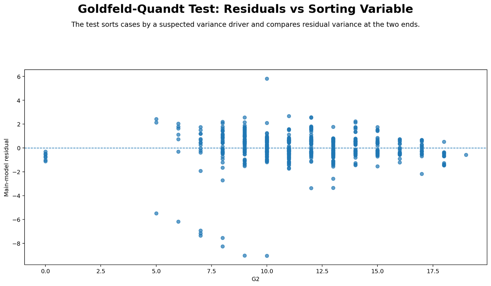
This chart plots the regression residuals against the chosen sort variable. In the verified analysis, the data were sorted by G2. The visual purpose is to check whether residual spread remains stable across the range of the sort variable. If the residual cloud has a similar vertical spread throughout the plot, that supports homoscedasticity. If the spread is wider in one region and narrower in another, that suggests heteroscedasticity.
The Goldfeld Quandt result confirms that residual variance was not constant. The lower sorted group had much higher residual mean squared error than the upper group. This means students with lower G2 values had more variable prediction errors for G3 than students with higher G2 values.
Decision/reporting conclusion: Report that the residuals-versus-sort-variable chart supports the formal Goldfeld Quandt decision because residual spread changes across G2, with stronger variance in the lower sorted group.
Python Chart 2: Lower and Upper Residual Boxplots
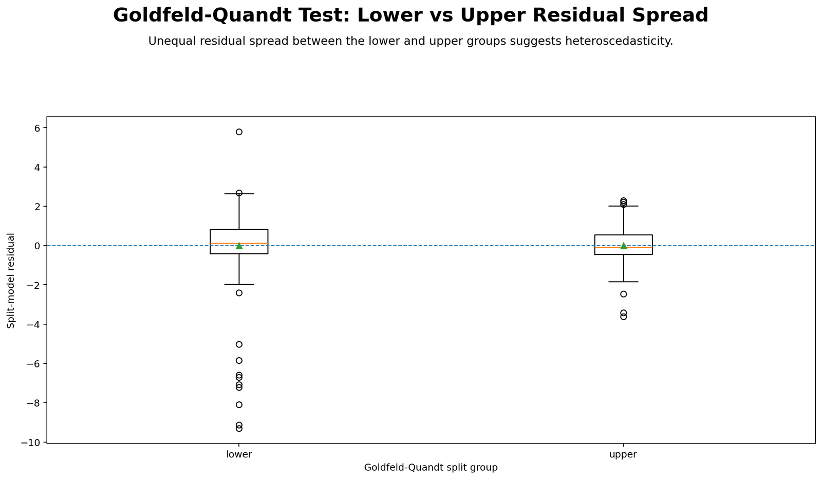
This chart compares residual distributions for the lower and upper groups after sorting. Boxplots make it easy to see differences in spread, median, interquartile range, and possible extreme residuals. In a homoscedastic model, the two groups should have roughly similar residual spread. In this analysis, the lower group residuals are more variable.
The formal output shows that lower group MSE was 2.94308, while upper group MSE was only .75661. That difference is large enough to produce F = 3.88982 and a significant p-value.
Decision/reporting conclusion: Report that the lower and upper residual boxplots visually support unequal variance. The lower sorted group has a wider residual distribution, consistent with significant heteroscedasticity.
Python Chart 3: Group Residual MSE
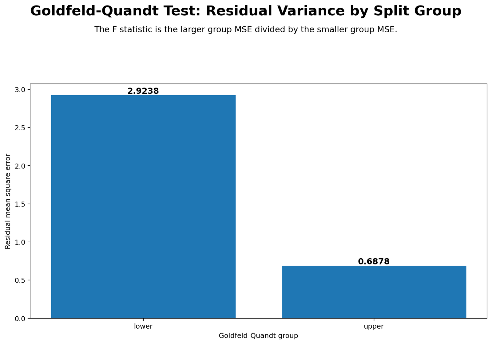
This chart directly visualizes the variance comparison used in the Goldfeld Quandt Test. The lower group residual MSE is visibly much larger than the upper group residual MSE. Numerically, the lower group MSE is 2.94308, while the upper group MSE is .75661.
This is the core diagnostic evidence. The Goldfeld Quandt F statistic is essentially the ratio of these two variance estimates. Because the ratio is large and statistically significant, the model does not satisfy the equal error variance assumption across the G2-sorted groups.
Decision/reporting conclusion: Report that the group residual MSE chart provides the clearest visual reason for rejecting homoscedasticity: the lower group error variance is nearly four times the upper group error variance.
Python Chart 4: Goldfeld Quandt p-value Decision
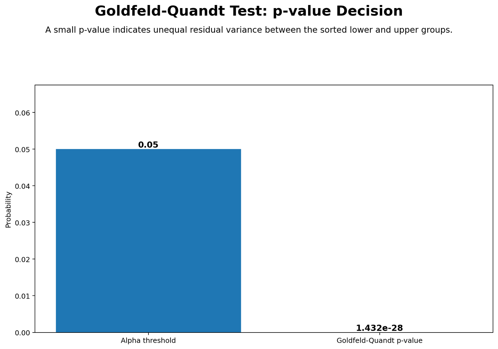
This chart translates the Goldfeld Quandt p-value into a decision. The p-value is reported as .0000, which should be interpreted as p < .001. Since this is below the standard .05 threshold, the null hypothesis of equal residual variance is rejected.
A p-value decision chart is useful for students because it separates the statistical decision from the practical interpretation. The decision is reject H0; the practical interpretation is that the regression has evidence of heteroscedasticity across the chosen sorted groups.
Decision/reporting conclusion: Report that the p-value decision chart confirms statistical significance. The model residual variance differs across G2-sorted groups, so the homoscedasticity assumption is not supported.
Python Chart 5: F Reference Curve
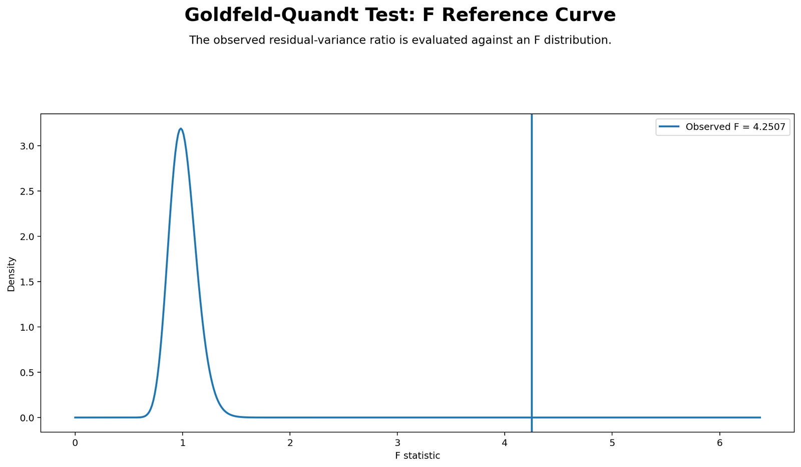
The F reference curve shows the Goldfeld Quandt test statistic relative to the F distribution. The statistic is F = 3.88982 with 253 and 253 degrees of freedom. Because the observed F statistic is far enough into the rejection region, the p-value becomes extremely small.
This chart is important because the Goldfeld Quandt Test is not just a visual comparison of variance. It is a formal F test. The F distribution tells us whether the observed variance ratio is larger than we would expect by random sampling variation under equal variance.
Decision/reporting conclusion: Report that the F reference curve supports rejection of the equal-variance null hypothesis because the observed F statistic falls in the statistically significant region.
Python Chart 6: Goldfeld Quandt Across Sort Variables
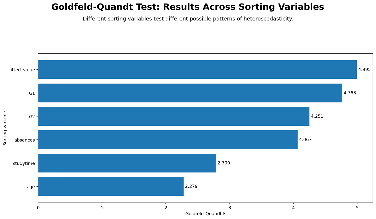
This chart compares Goldfeld Quandt results across different possible sorting variables. It helps answer an important diagnostic question: is heteroscedasticity mainly associated with one variable, or does it appear across several sorting choices? Because the Goldfeld Quandt Test depends on the sort variable, this chart prevents the analyst from overgeneralizing from only one split.
In the verified SPSS result, the main reported sort variable is G2. The cross-variable chart is useful as a sensitivity check because regression residual variance may change across fitted values, previous grades, absences, or other predictors.
Decision/reporting conclusion: Report that the across-sort-variables chart should be used as a diagnostic comparison. The confirmed SPSS result sorted by G2 is significant, and other sort variables should be interpreted as supporting or sensitivity evidence.
Python Chart 7: Residuals vs Fitted Values
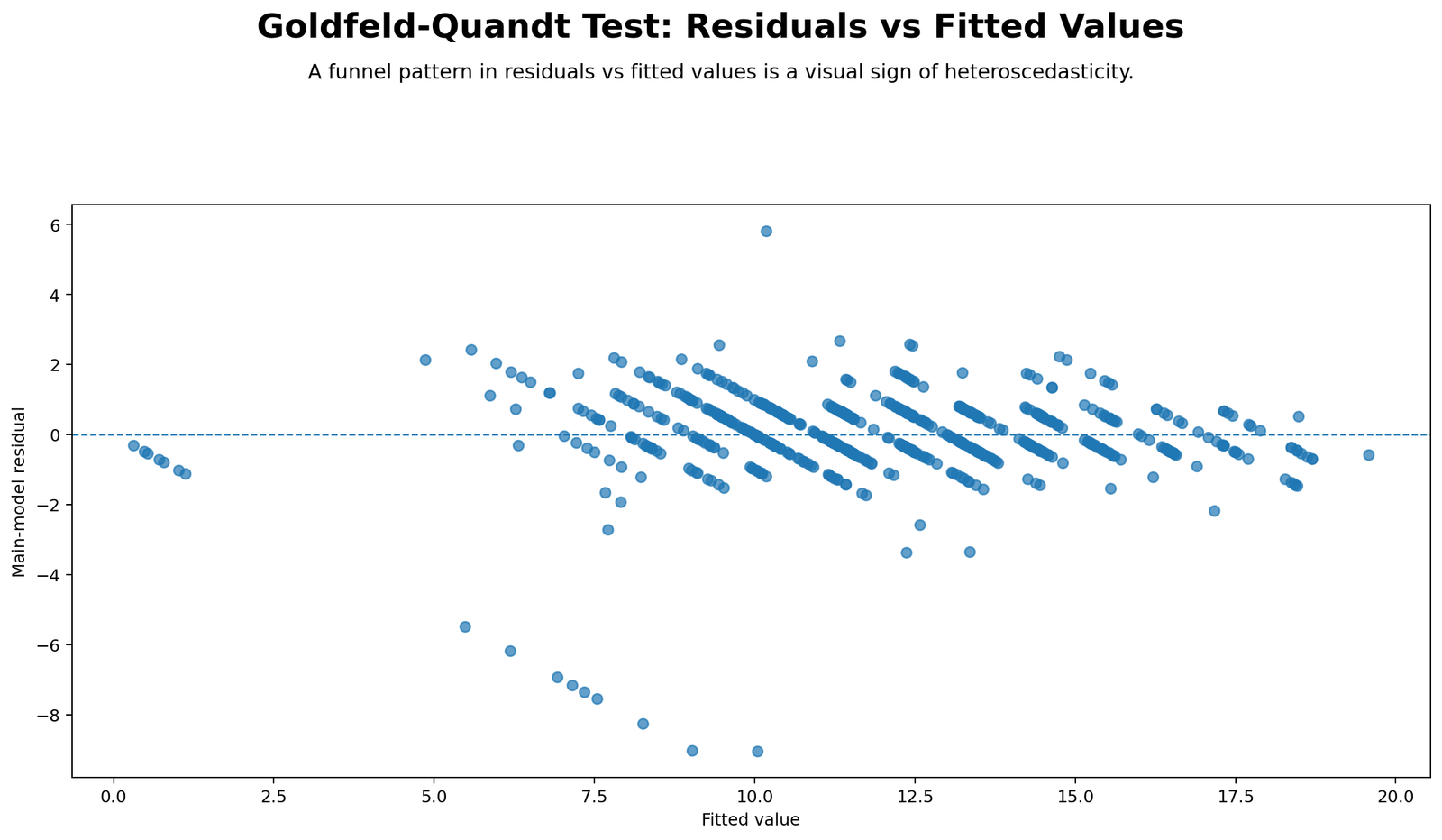
The residuals-versus-fitted-values chart is a standard regression diagnostic plot. It checks whether residual spread changes as predicted values increase. If the residuals show a funnel shape, curve, or systematic pattern, the model may have heteroscedasticity, nonlinearity, or specification problems.
In this analysis, the Goldfeld Quandt Test already provides formal evidence of unequal variance. The residuals-versus-fitted chart helps explain whether the problem also appears across predicted G3 values, not only across the G2-sorted split.
Decision/reporting conclusion: Report that the residuals-versus-fitted chart should be used with the Goldfeld Quandt result. The formal test rejects homoscedasticity, and the fitted-value plot helps diagnose the location and pattern of unequal variance.
R Chart-by-Chart Validation
The R charts validate the same Goldfeld Quandt Test workflow using a separate software environment. They confirm the Python and SPSS story: the regression model is strong, but the residual variance is not equal across the sorted groups.
R Chart 1: Residuals vs Sort Variable
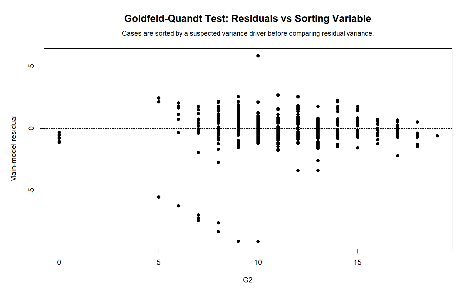
The R residuals-versus-sort-variable chart validates the same diagnostic pattern shown in Python. It checks whether residual spread remains equal across the sorting variable. When the residual spread changes from one region of the sorted variable to another, heteroscedasticity becomes plausible.
Because the verified result sorted by G2 is significant, this R chart supports the conclusion that residual variance is not stable across the G2-sorted data.
Decision/reporting conclusion: Report that the R residual plot validates the Python and SPSS evidence: residual variance changes across the sort variable, supporting heteroscedasticity.
R Chart 2: Lower and Upper Residual Boxplots
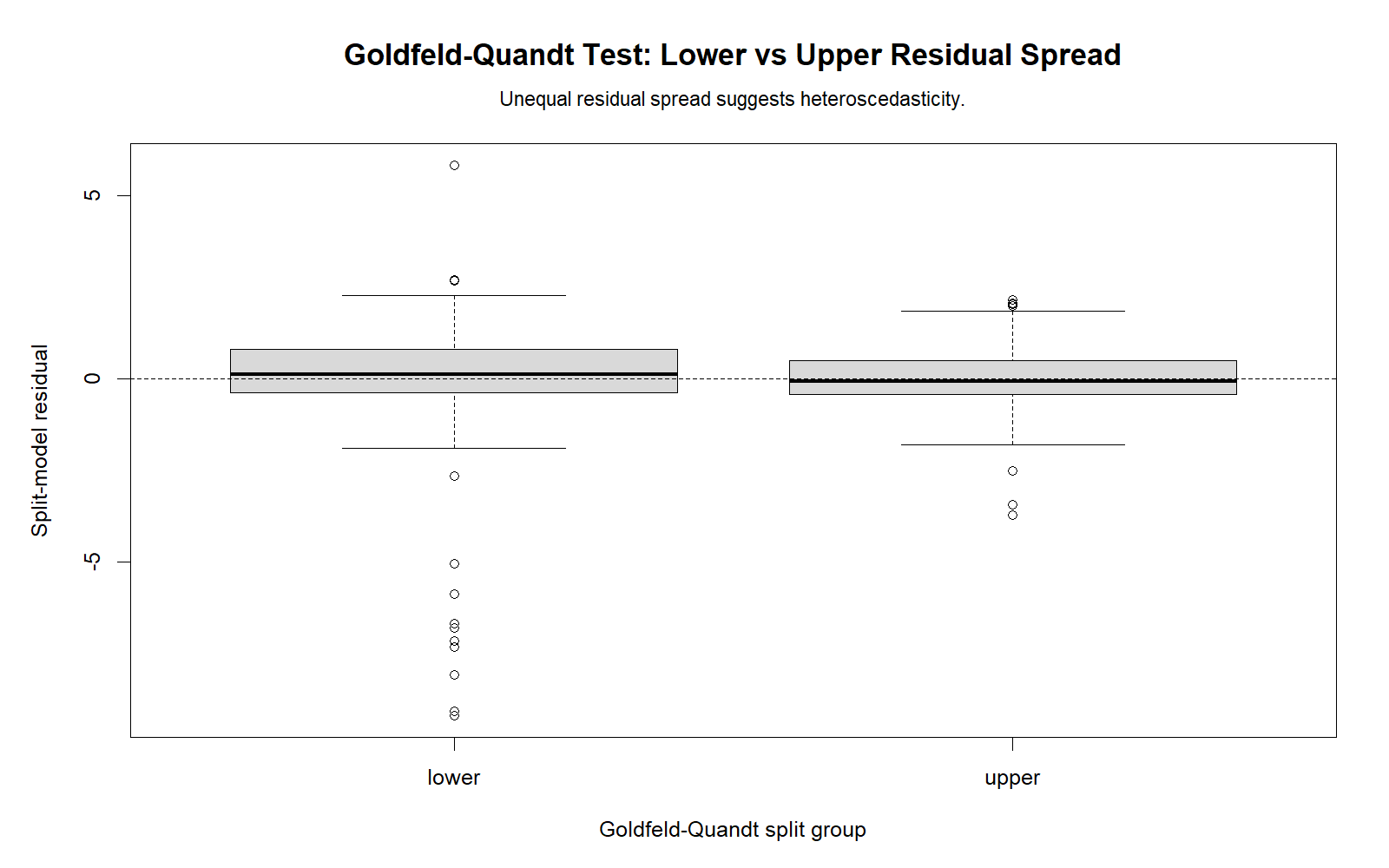
The R lower and upper residual boxplots provide a clear visual comparison of spread. In a homoscedastic model, both boxplots should have similar vertical spread. The verified output shows that the lower group variance is much larger than the upper group variance, and the R boxplots validate that diagnostic difference.
Decision/reporting conclusion: Report that the R boxplots confirm unequal residual spread between lower and upper groups, supporting the formal rejection of homoscedasticity.
R Chart 3: Group Residual MSE
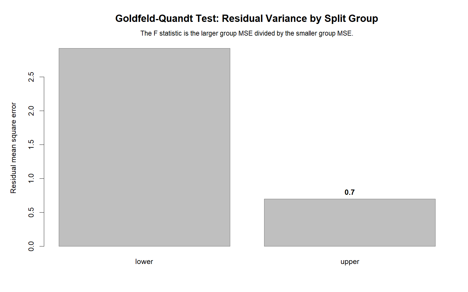
This R chart validates the central numerical comparison in the Goldfeld Quandt Test. It shows that the lower group residual MSE is greater than the upper group residual MSE. The verified SPSS values are 2.94308 for the lower group and .75661 for the upper group.
Decision/reporting conclusion: Report that R confirms the group-MSE imbalance. The lower group has substantially greater residual variance, which produces the significant Goldfeld Quandt F statistic.
R Chart 4: Goldfeld Quandt p-value Decision
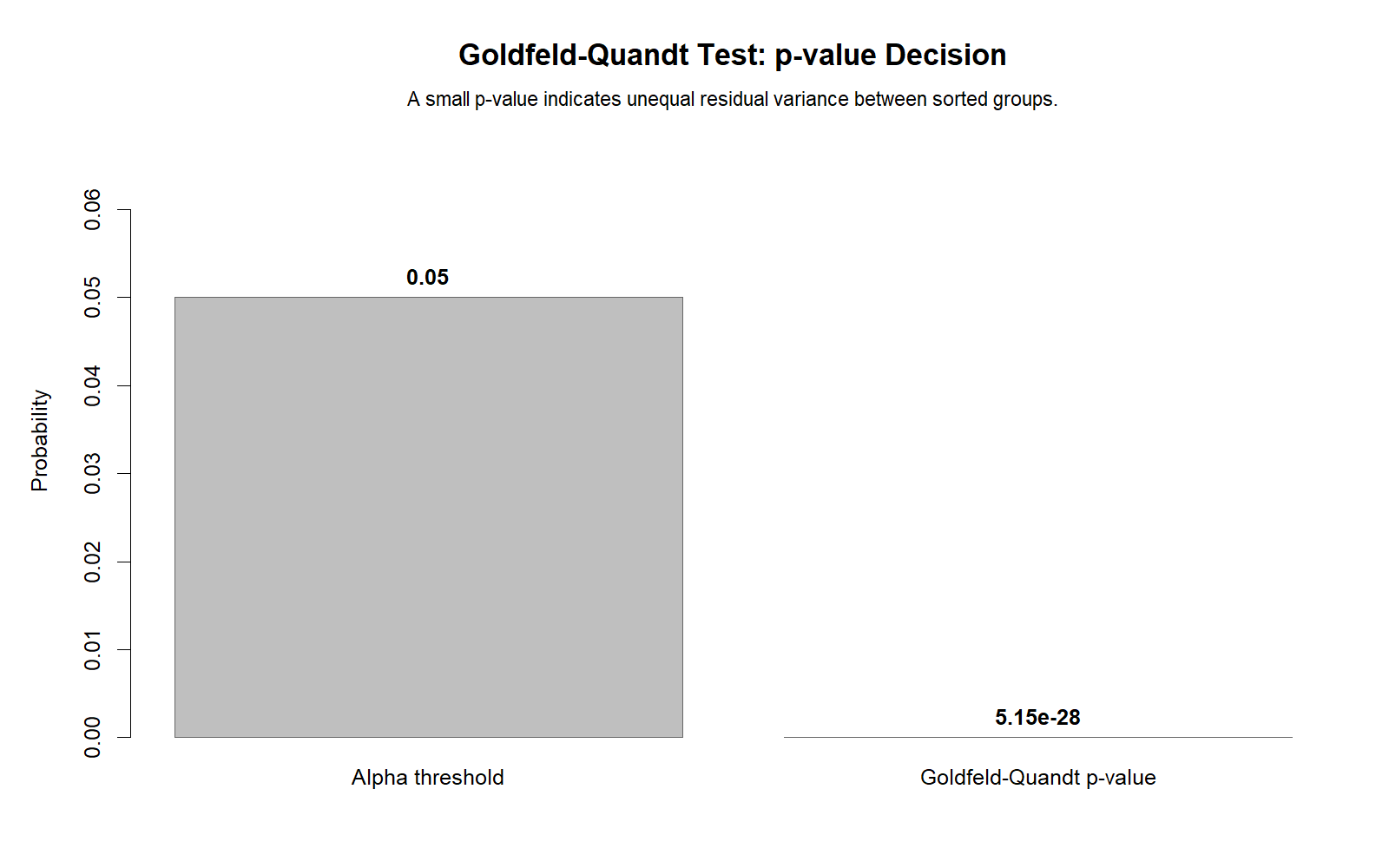
The R p-value decision chart confirms the same formal conclusion. The p-value is below .05, so the null hypothesis of equal residual variance is rejected. Since the SPSS p-value is reported as .0000, the result should be written as p < .001 in the final report.
Decision/reporting conclusion: Report that R validates the statistical decision: the Goldfeld Quandt Test is significant and heteroscedasticity is present.
R Chart 5: F Reference Curve
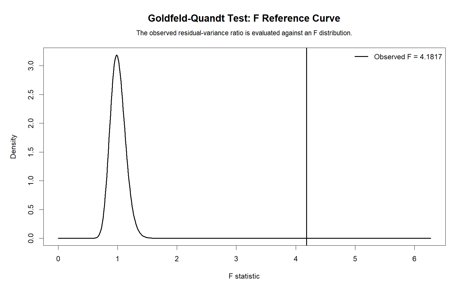
The R F reference curve validates the formal test distribution. The observed F value, 3.88982, is evaluated against an F distribution with 253 and 253 degrees of freedom. The result falls in the rejection region, confirming that the variance ratio is too large to treat as random variation under equal variance.
Decision/reporting conclusion: Report that the R F curve confirms the Goldfeld Quandt statistic is statistically significant, supporting rejection of the homoscedasticity assumption.
R Chart 6: Goldfeld Quandt Across Sort Variables
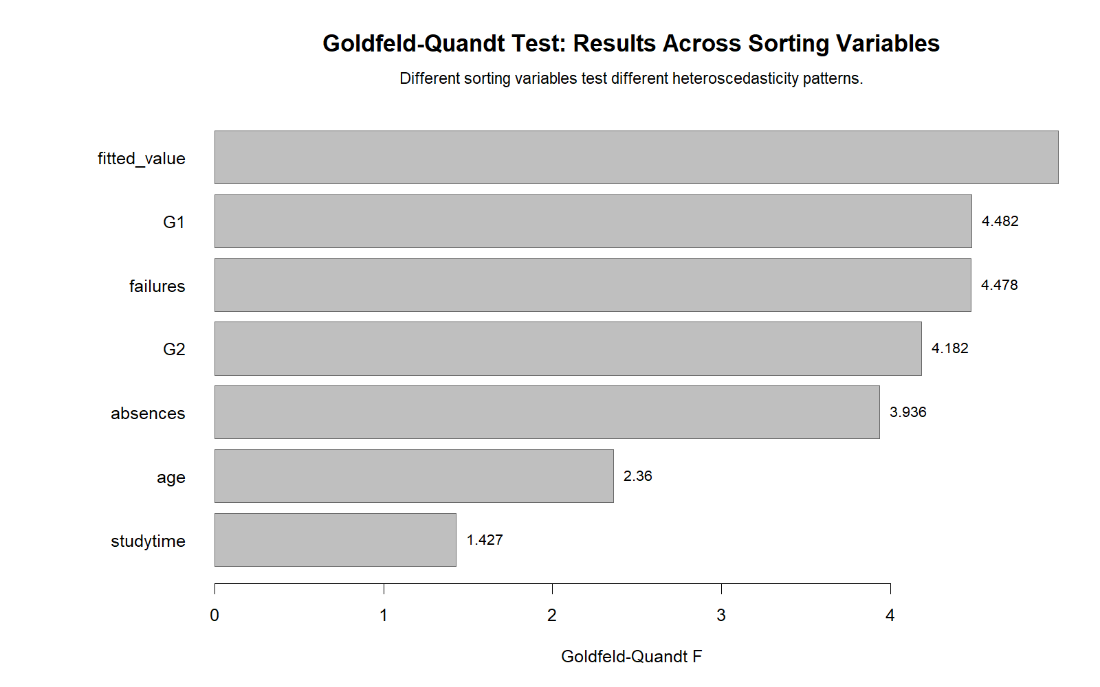
The R across-sort-variables chart validates the sensitivity-check approach. Since the Goldfeld Quandt Test depends on how the data are sorted, it is useful to compare possible sort variables rather than relying blindly on one variable. This does not replace the verified G2-based SPSS result, but it helps interpret whether the heteroscedasticity pattern is broad or variable-specific.
Decision/reporting conclusion: Report that the R across-sort-variables chart supports diagnostic transparency. The main confirmed decision is based on sorting by G2, while other sort variables can be discussed as sensitivity checks.
R Chart 7: Residuals vs Fitted Values
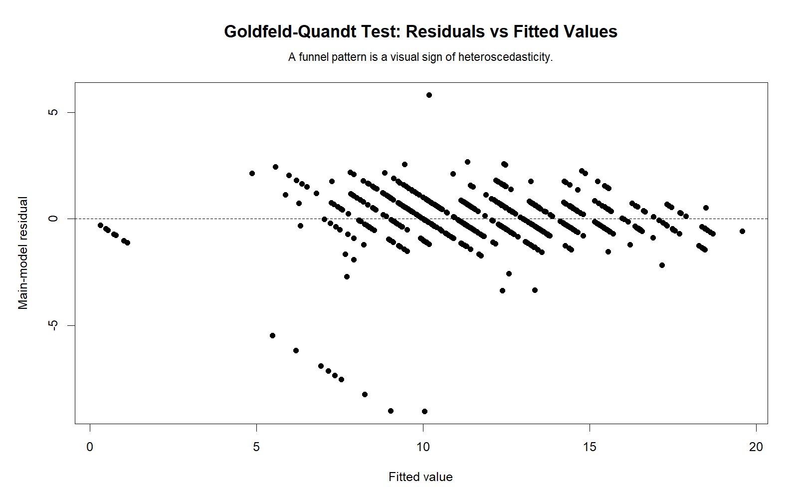
The R residuals-versus-fitted-values chart validates the general regression diagnostic picture. A random and evenly spread residual cloud supports model assumptions, while changing spread, fan shapes, or systematic patterns suggest possible heteroscedasticity or misspecification.
Because the Goldfeld Quandt Test is significant, this plot should be interpreted as supporting diagnostic evidence. It helps show where residual variance may be changing across the fitted-value range.
Decision/reporting conclusion: Report that the R residuals-versus-fitted chart should be interpreted together with the significant Goldfeld Quandt Test. The formal result indicates heteroscedasticity, and the residual plot helps diagnose its pattern.
SPSS, Python, R and Excel Workflows for the Goldfeld Quandt Test
The Goldfeld Quandt workflow is similar across software. First, fit the regression model. Second, save residuals and predicted values. Third, sort the data by a suspected scale variable. Fourth, remove or ignore the middle group if using the classic Goldfeld Quandt split. Fifth, compare lower and upper residual mean squared errors using an F statistic.
SPSS Workflow
| Step | SPSS Action | Purpose |
|---|---|---|
| Open dataset | File > Open > Data | Load the SPSS-ready dataset. |
| Fit main regression | Analyze > Regression > Linear | Predict G3 using G1, G2, studytime, failures, and absences. |
| Save residuals | Save > Unstandardized Residuals | Create residual variable for diagnostics. |
| Square residuals | Transform > Compute Variable | Create squared residuals for variance comparison. |
| Sort by G2 | Data > Sort Cases | Create lower, middle, and upper sorted groups. |
| Compare variance groups | Means, Aggregate, or custom syntax | Calculate lower and upper residual MSE. |
| Calculate F statistic | Compute lower MSE ÷ upper MSE | Get Goldfeld Quandt F statistic. |
| Export output | OUTPUT EXPORT | Save verified SPSS output PDF. |
Python Workflow
| Step | Python Action | Purpose |
|---|---|---|
| Read data | pandas.read_csv() | Load the dataset. |
| Fit regression model | statsmodels.OLS() | Estimate the main regression model. |
| Extract residuals | model.resid | Use residuals for heteroscedasticity diagnostics. |
| Sort cases | sort_values("G2") | Sort observations by the suspected scale variable. |
| Split groups | Lower, middle, upper groups | Omit middle group and compare lower versus upper. |
| Calculate F | max(mse1,mse2)/min(mse1,mse2) | Calculate Goldfeld Quandt statistic. |
| Calculate p-value | scipy.stats.f.sf() | Test whether the variance ratio is significant. |
R Workflow
| Step | R Action | Purpose |
|---|---|---|
| Read data | read.csv() | Load the dataset. |
| Fit regression model | lm(G3 ~ G1 + G2 + studytime + failures + absences) | Estimate OLS regression. |
| Extract residuals | resid(model) | Create residual diagnostic variable. |
| Sort by G2 | order(df$G2) | Prepare lower and upper comparison groups. |
| Calculate group MSE | mean(residuals^2) | Estimate residual variance by group. |
| Run formal test | lmtest::gqtest() | Use a standard R implementation of the Goldfeld Quandt Test. |
Excel Workflow
| Excel Task | Formula or Tool | Purpose |
|---|---|---|
| Fit regression | Data Analysis ToolPak > Regression | Estimate predicted G3 values. |
| Calculate residuals | =Observed-Predicted | Create residual variable. |
| Square residuals | =Residual^2 | Create squared residuals for MSE comparison. |
| Sort by G2 | Data > Sort | Sort cases by the suspected scale variable. |
| Calculate lower MSE | =AVERAGE(lower squared residual range) | Estimate residual variance in lower group. |
| Calculate upper MSE | =AVERAGE(upper squared residual range) | Estimate residual variance in upper group. |
| Calculate F | =MAX(lower_mse,upper_mse)/MIN(lower_mse,upper_mse) | Calculate Goldfeld Quandt statistic. |
| Calculate p-value | =F.DIST.RT(F,df1,df2) | Determine whether the variance ratio is significant. |
SPSS Syntax, Python Code, R Code and Excel Formulas
SPSS Syntax for Goldfeld Quandt Test
* Goldfeld Quandt Test in SPSS.
* Model: G3 predicted by G1, G2, studytime, failures, and absences.
* Sort variable: G2.

SET PRINTBACK=OFF MPRINT=OFF.

TITLE "Goldfeld Quandt Test: Regression and Heteroscedasticity Diagnostic".

REGRESSION
  /DEPENDENT G3
  /METHOD=ENTER G1 G2 studytime failures absences
  /SAVE PRED(gq_pred) RESID(gq_resid)
  /STATISTICS COEFF OUTS R ANOVA CI(95).

COMPUTE gq_sq_resid = gq_resid ** 2.
EXECUTE.

SORT CASES BY G2(A).

* Example group coding for 649 cases:
* Lower group = first 259 sorted cases.
* Middle group = next 131 cases.
* Upper group = final 259 cases.
* Adjust case numbers if your sample size changes.

COMPUTE case_order = $CASENUM.
IF (case_order LE 259) gq_group = 1.
IF (case_order GT 259 AND case_order LE 390) gq_group = 0.
IF (case_order GT 390) gq_group = 2.
EXECUTE.

MEANS TABLES=gq_resid gq_sq_resid BY gq_group
  /CELLS=COUNT MEAN STDDEV VARIANCE.

* Residual diagnostics.
EXAMINE VARIABLES=gq_resid
  /PLOT BOXPLOT HISTOGRAM NPPLOT
  /STATISTICS DESCRIPTIVES
  /CINTERVAL 95
  /MISSING LISTWISE
  /NOTOTAL.

CORRELATIONS
  /VARIABLES=gq_resid gq_sq_resid gq_pred G2 absences
  /PRINT=TWOTAIL NOSIG
  /MISSING=PAIRWISE.

OUTPUT SAVE OUTFILE="Goldfeld-Quandt-Test-SPSS-Output.spv".

OUTPUT EXPORT
  /CONTENTS EXPORT=VISIBLE
  /PDF DOCUMENTFILE="Goldfeld-Quandt-Test-SPSS-Output.pdf".
Python Code for Goldfeld Quandt Test
import pandas as pd
import numpy as np
import statsmodels.api as sm
from scipy import stats

df = pd.read_csv("dataset.csv")

target = "G3"
predictors = ["G1", "G2", "studytime", "failures", "absences"]
sort_variable = "G2"

data = df[[target] + predictors].dropna().copy()

X = sm.add_constant(data[predictors])
y = data[target]

model = sm.OLS(y, X).fit()

data["gq_pred"] = model.fittedvalues
data["gq_resid"] = model.resid
data["gq_sq_resid"] = data["gq_resid"] ** 2

sorted_data = data.sort_values(sort_variable).reset_index(drop=True)

n = len(sorted_data)
lower_n = 259
middle_n = 131
upper_n = 259

lower = sorted_data.iloc[:lower_n]
upper = sorted_data.iloc[-upper_n:]

k = len(predictors) + 1

lower_mse = np.sum(lower["gq_resid"] ** 2) / (lower_n - k)
upper_mse = np.sum(upper["gq_resid"] ** 2) / (upper_n - k)

gq_f = max(lower_mse, upper_mse) / min(lower_mse, upper_mse)
df_num = lower_n - k
df_den = upper_n - k
p_value = stats.f.sf(gq_f, df_num, df_den)

print(model.summary())
print("Lower MSE:", lower_mse)
print("Upper MSE:", upper_mse)
print("Goldfeld-Quandt F:", gq_f)
print("df numerator:", df_num)
print("df denominator:", df_den)
print("p-value:", p_value)

if p_value < 0.05:
    print("Reject H0: evidence of heteroscedasticity.")
else:
    print("Fail to reject H0: no significant evidence of heteroscedasticity.")
R Code for Goldfeld Quandt Test
# Goldfeld Quandt Test in R

df <- read.csv("dataset.csv")

model <- lm(G3 ~ G1 + G2 + studytime + failures + absences, data = df)
summary(model)

df$gq_pred <- fitted(model)
df$gq_resid <- resid(model)
df$gq_sq_resid <- df$gq_resid^2

df_sorted <- df[order(df$G2), ]

lower_n <- 259
middle_n <- 131
upper_n <- 259

lower <- df_sorted[1:lower_n, ]
upper <- df_sorted[(nrow(df_sorted) - upper_n + 1):nrow(df_sorted), ]

k <- length(coef(model))

lower_mse <- sum(lower$gq_resid^2) / (lower_n - k)
upper_mse <- sum(upper$gq_resid^2) / (upper_n - k)

gq_f <- max(lower_mse, upper_mse) / min(lower_mse, upper_mse)
df_num <- lower_n - k
df_den <- upper_n - k
p_value <- pf(gq_f, df_num, df_den, lower.tail = FALSE)

cat("Lower MSE:", lower_mse, "\n")
cat("Upper MSE:", upper_mse, "\n")
cat("Goldfeld-Quandt F:", gq_f, "\n")
cat("df numerator:", df_num, "\n")
cat("df denominator:", df_den, "\n")
cat("p-value:", p_value, "\n")

# Optional standard package implementation
# install.packages("lmtest")
library(lmtest)
gqtest(model, order.by = ~ G2, data = df)
Excel Formulas for Goldfeld Quandt Test
Assume:
Observed G3 is in column A.
Predicted G3 is in column B.
Residual is in column C.
Squared residual is in column D.
G2 sort variable is in column E.

Residual:
=A2-B2

Squared residual:
=C2^2

Sort all rows by G2 from smallest to largest.

Lower group MSE:
=SUM(lower_squared_residual_range)/(lower_n-k)

Upper group MSE:
=SUM(upper_squared_residual_range)/(upper_n-k)

Goldfeld Quandt F statistic:
=MAX(lower_mse,upper_mse)/MIN(lower_mse,upper_mse)

Degrees of freedom:
df1 = lower_n-k
df2 = upper_n-k

p-value:
=F.DIST.RT(F_statistic,df1,df2)

Decision:
If p-value < 0.05, reject equal variance.
If p-value ≥ 0.05, fail to reject equal variance.

Example from this guide:
Lower MSE = 2.94308
Upper MSE = 0.75661
F = 2.94308 / 0.75661 = 3.88982
df1 = 253
df2 = 253
p-value < .001
Decision: Reject homoscedasticity.
APA Reporting Wording for the Goldfeld Quandt Test
When reporting the Goldfeld Quandt Test, include the dependent variable, model predictors, sort variable, lower and upper residual variance estimates, F statistic, degrees of freedom, p-value, and conclusion about heteroscedasticity.
APA-Style Goldfeld Quandt Report
A Goldfeld Quandt Test was conducted to evaluate heteroscedasticity in the regression model predicting G3 from G1, G2, studytime, failures, and absences. The data were sorted by G2, and residual mean squared errors were compared between the lower and upper groups. The lower group had a larger residual mean squared error, MSE = 2.94308, than the upper group, MSE = .75661. The Goldfeld Quandt Test was significant, F(253, 253) = 3.88982, p < .001, indicating unequal residual variance across the G2-sorted groups. Therefore, the homoscedasticity assumption was not supported.
Short Report Sentence
The Goldfeld Quandt Test indicated significant heteroscedasticity when residuals were sorted by G2, F(253, 253) = 3.88982, p < .001. The lower G2 group showed higher residual variance than the upper G2 group.
Student-Friendly Report Example
The regression model predicted G3 well, but the Goldfeld Quandt Test showed that the model errors were not equally spread across G2 groups. The lower G2 group had much larger residual variance than the upper G2 group. Since the p-value was below .05, the equal variance assumption was rejected.
When writing the final results section, connect the assumption result with practical interpretation. If you report coefficients, also discuss uncertainty using confidence intervals and practical importance using effect size. If a one-directional research question is involved in a separate hypothesis test, see the one-tailed t-test guide. For z-based tests, Salar Cafe also provides guides on the one-sample z-test and one-proportion z-test.
Common Mistakes in Goldfeld Quandt Test Interpretation
| Mistake | Why It Is a Problem | Correct Practice |
|---|---|---|
| Ignoring the sort variable | The Goldfeld Quandt result depends on how the data are sorted. | Always report the sort variable, such as G2 in this example. |
| Calling the test a normality test | Goldfeld Quandt tests unequal residual variance, not residual normality. | Use Q-Q plots, P-P plots, Shapiro-Wilk, or related tests for normality. |
| Only reporting the p-value | The p-value does not show which group has larger variance. | Report lower and upper MSE values with the F statistic. |
| Forgetting model specification | Heteroscedasticity may be caused by missing nonlinear terms or misspecification. | Check residual plots and consider the Ramsey RESET test. |
| Assuming heteroscedasticity invalidates everything | The model may still be useful, but inference may need correction. | Consider robust standard errors, transformations, or weighted least squares. |
| Using all observations without a clear split rule | The classic Goldfeld Quandt approach often omits a middle group. | State group sizes and middle omission rule clearly. |
| Confusing residual variance with predictor variance | The test compares error variance, not simply spread in the predictor. | Compute residuals from the regression model first, then compare residual variance. |
Key reminder: The Goldfeld Quandt Test should be interpreted with residual plots and model knowledge. A significant result tells you unequal residual variance exists across the chosen split, but it does not automatically tell you the best correction.
When to Use the Goldfeld Quandt Test
Use the Goldfeld Quandt Test when you have a regression model and you suspect that residual variance changes across a specific variable. It is especially useful when theory suggests that errors may be larger for low or high values of a predictor.
| Use Case | Why the Goldfeld Quandt Test Helps | Example from This Guide |
|---|---|---|
| Regression assumption checking | Tests whether residual variance is equal across sorted groups. | Residuals from the G3 regression model were sorted by G2. |
| Suspected heteroscedasticity | Formalizes what residual plots suggest visually. | Lower G2 group had much larger residual variance. |
| Comparing lower and upper error variance | Uses an F ratio of residual MSE values. | F = 2.94308 ÷ .75661 = 3.88982. |
| Model diagnostics before final reporting | Helps decide whether robust standard errors or model changes are needed. | Significant p-value indicates inference may need adjustment. |
| Sensitivity checking across sort variables | Shows whether heteroscedasticity depends on the chosen sort variable. | Python and R charts compare Goldfeld Quandt results across sort variables. |
If your data involve repeated-measures assumptions instead of regression error variance, see Mauchly’s test of sphericity and Greenhouse-Geisser correction. If your research uses categorical summaries, the cross-tabulation guide may be more relevant than regression diagnostics. For applied biomedical examples in R, see clinical trial data analysis using R.
Downloads and Resources for Goldfeld Quandt Test
The resources below include the verified SPSS output PDF, Python charts, and R validation charts used in this Goldfeld Quandt Test guide.
Download SPSS Output PDF
Verified SPSS output for regression model, residual diagnostics, Goldfeld Quandt split, F statistic and p-value decision.
Copy Goldfeld Quandt Code
Use the SPSS, Python, R and Excel code blocks to reproduce the heteroscedasticity workflow.
Python Chart 1: Residuals vs Sort Variable
Visual diagnostic chart showing residual spread across the sort variable.
Python Chart 3: Group Residual MSE
Lower and upper group residual mean squared error comparison.
R Chart 3: Group Residual MSE
R validation chart confirming residual MSE difference by group.
R Chart 5: F Reference Curve
F distribution chart for interpreting the Goldfeld Quandt statistic.
FAQs About the Goldfeld Quandt Test
What is the Goldfeld Quandt Test?
The Goldfeld Quandt Test is a regression diagnostic test for heteroscedasticity. It checks whether residual variance differs between lower and upper groups after sorting the data by a chosen variable.
What does the Goldfeld Quandt Test measure?
It measures whether residual error variance is equal across two sorted groups. A significant result suggests unequal variance, also called heteroscedasticity.
What was the Goldfeld Quandt Test result in this guide?
The verified result was F(253, 253) = 3.88982, p < .001. Therefore, the null hypothesis of equal residual variance was rejected.
What was the sort variable in this Goldfeld Quandt Test?
The main sort variable was G2. Residuals were compared between lower and upper groups after sorting the data by G2.
Which group had larger residual variance?
The lower G2-sorted group had larger residual variance. Its MSE was 2.94308, compared with .75661 for the upper group.
What is the null hypothesis of the Goldfeld Quandt Test?
The null hypothesis is that residual variance is equal between the lower and upper sorted groups. In this example, the null was rejected.
Is the Goldfeld Quandt Test a normality test?
No. It is a heteroscedasticity test. For normality, use Q-Q plots, P-P plots, Shapiro-Wilk, Kolmogorov-Smirnov, Lilliefors, D’Agostino-Pearson, or Ryan-Joiner checks.
What should I do if the Goldfeld Quandt Test is significant?
Consider robust standard errors, weighted least squares, transformations, alternative model specifications, or additional diagnostics such as residual plots and the Ramsey RESET test.
Can I run the Goldfeld Quandt Test in Excel?
Yes. Fit the regression, calculate residuals, square residuals, sort by the suspected variable, calculate lower and upper MSE values, compute the F ratio, and use F.DIST.RT to calculate the p-value.
How do I report the Goldfeld Quandt Test in APA style?
Report the model, sort variable, group MSE values, F statistic, degrees of freedom, p-value, and conclusion. For this guide: the Goldfeld Quandt Test was significant, F(253, 253) = 3.88982, p < .001, indicating heteroscedasticity.

