
ANOVA effect size, formula and worked example
Cohen’s f: Formula, ANOVA Effect Size & Examples
Cohen’s f is a standardized ANOVA effect size used for interpretation and power analysis. Learn the formula, convert eta squared or partial eta squared, interpret thresholds, and follow a verified worked example.
Quick Answer: Cohen’s F Result
The worked Cohen’s F example converts ANOVA effect-size values into Cohen’s f for the studytime effect on G3 final grade. The group mean chart shows that mean G3 is lowest in studytime group 1, higher in group 2, highest in group 3 and still high in group 4. The same group pattern appears in the boxplot and the ANOVA F distribution chart.
The conversion chart reports Cohen’s f = 0.2717 from eta squared and partial eta squared. It also reports Cohen’s f = 0.2622 from omega squared and Cohen’s f = 0.2624 from epsilon squared. The threshold chart places the observed Cohen’s f near 0.272, which is above the medium threshold of 0.25 and below the large threshold of 0.40.
Final interpretation: Cohen’s f is about 0.272 for the studytime effect on G3. This value is above the medium threshold of 0.25 and below the large threshold of 0.40, so the effect is interpreted as medium. Studytime explains about 6.9% of the variation in G3, while about 93.1% remains unexplained or within-group variation.
Important reporting point: Cohen’s f is not the same as the ANOVA F statistic. The ANOVA F statistic tests whether group means differ statistically. Cohen’s f reports the practical size of the group effect after converting explained variance to a standardized effect-size scale.
Table of Contents
- What Is Cohen’s F?
- Cohen’s F Formula
- Statistical Decision and Effect-Size Interpretation
- Dataset and Variables Used
- Python Chart-by-Chart Interpretation
- R Chart-by-Chart Validation
- SPSS Output Interpretation
- SPSS, R, Python and Excel Workflows
- Code Blocks for Cohen’s F
- APA Reporting Wording
- Common Mistakes
- When to Use Cohen’s F
- Downloads and Resources
- Related Guides
- FAQs
What Is Cohen’s F?
Cohen’s F is an ANOVA-family effect-size measure. It expresses the practical size of a group effect on a standardized scale. Instead of reporting only the percentage of variance explained, Cohen’s f converts the explained variance into a value that can be interpreted with small, medium and large reference points.
In this example, Cohen’s f summarizes the effect of studytime on G3 final grade. The ANOVA result shows that studytime groups differ statistically, and the variance explained chart shows that studytime explains about 6.9% of G3 variation. Cohen’s f converts that explained variance into an observed value of about 0.272.
The interpretation threshold chart uses 0.10 for a small effect, 0.25 for a medium effect and 0.40 for a large effect. The observed value of 0.272 sits just above the medium threshold. This means the studytime effect should be reported as medium, not small and not large.
Simple definition: Cohen’s f is an ANOVA effect-size measure. In this output, Cohen’s f is about 0.272, which means the studytime effect on G3 is medium in practical size.
Cohen’s f should be interpreted with Effect Size, ANOVA Effect Size, ANOVA in Python, ANOVA in R, ANOVA in SPSS, ANOVA Assumptions, Statistical Power, P Value, Null and Alternative Hypothesis and Type I and Type II Error.
Cohen’s F Formula
Cohen’s f is usually calculated from an explained-variance effect size. The most common conversion uses eta squared or partial eta squared.
When eta squared is used, the formula converts the proportion of total variance explained into Cohen’s f. In this output, eta squared is about .0688 to .069, so Cohen’s f becomes about 0.2717.
Cohen’s f from Partial Eta Squared
When partial eta squared is used, the same conversion is applied. In this one-way ANOVA example, eta squared and partial eta squared are the same or nearly the same, so both conversions give Cohen’s f = 0.2717.
Cohen’s f from Omega Squared
Omega squared is a more conservative explained-variance estimate. Because omega squared is slightly smaller than eta squared, the resulting Cohen’s f is also slightly smaller. The conversion summary chart reports Cohen’s f = 0.2622 from omega squared.
Cohen’s f from Epsilon Squared
Epsilon squared gives another adjusted explained-variance estimate. The conversion summary chart reports Cohen’s f = 0.2624 from epsilon squared, which is very close to the omega-based conversion.
| Conversion Source | Cohen’s f Value | Meaning | Interpretation |
|---|---|---|---|
| Eta squared | 0.2717 | Conversion from total explained variance. | Medium effect. |
| Partial eta squared | 0.2717 | Conversion from effect-plus-error explained variance. | Medium effect. |
| Omega squared | 0.2622 | Conversion from adjusted explained variance. | Medium effect. |
| Epsilon squared | 0.2624 | Conversion from another adjusted explained-variance estimate. | Medium effect. |
| Observed threshold chart | 0.272 | Displayed observed Cohen’s f. | Above medium threshold and below large threshold. |
Statistical Decision and Effect-Size Interpretation
Cohen’s f does not test the null hypothesis by itself. The ANOVA F statistic tests whether group means differ statistically. Cohen’s f explains how large the group effect is after the ANOVA model has been fitted.
| Question | Statistic | Value in This Output | Interpretation |
|---|---|---|---|
| Do studytime group means differ? | ANOVA F statistic | Observed F = 15.88, critical F = 2.62 | The group difference is statistically significant. |
| How much variance is explained? | Eta squared / variance explained | About 6.9% | Studytime explains a meaningful part of G3 variation. |
| How large is the standardized effect? | Cohen’s f | About 0.272 | Medium effect. |
| Is the effect large? | Threshold comparison | Observed 0.272 below large threshold 0.40 | The effect is medium, not large. |
Decision for this example: The ANOVA F statistic shows a statistically significant studytime effect on G3, and Cohen’s f shows that the practical size of the effect is medium. The result should be reported as significant and medium-sized, with Cohen’s f around 0.27.
Dataset and Variables Used
The worked example uses a student performance dataset. The dependent variable is G3 final grade, and the grouping factor is studytime. The ANOVA compares mean G3 across four studytime groups and then converts the effect-size values into Cohen’s f.
| Variable or Output | Role | Why It Matters for Cohen’s f | Where It Appears |
|---|---|---|---|
| G3 | Dependent variable | Final grade outcome being compared. | Group means, boxplot, ANOVA model and variance explained. |
| studytime | Grouping factor | Explains part of the variation in G3. | Group mean chart and variance explained pie chart. |
| Eta squared | Explained variance | Used to calculate Cohen’s f. | Conversion summary and effect size comparison. |
| Omega squared | Adjusted explained variance | Produces a slightly more conservative Cohen’s f. | Conversion summary. |
| ANOVA F statistic | Significance test | Shows that group means differ statistically. | F distribution curve. |
| Cohen’s f | Standardized effect size | Shows practical magnitude and supports power analysis. | Conversion chart and threshold chart. |
For supporting concepts, review Descriptive Statistics, Mean Median and Mode, Standard Deviation, Variance, Standard Error, Confidence Interval, Coefficient of Variation, Frequency Distribution, Five Number Summary, Percentiles and Quartiles, Interquartile Range, Range, Skewness and Kurtosis.
Python Chart-by-Chart Interpretation
The Python charts below show the first Cohen’s f workflow. They explain the group mean pattern, conversion from ANOVA effect sizes, comparison among effect-size measures, ANOVA F decision, variance explained, group distribution and interpretation thresholds.
Python Chart 1: Group Means with 95% Confidence Intervals
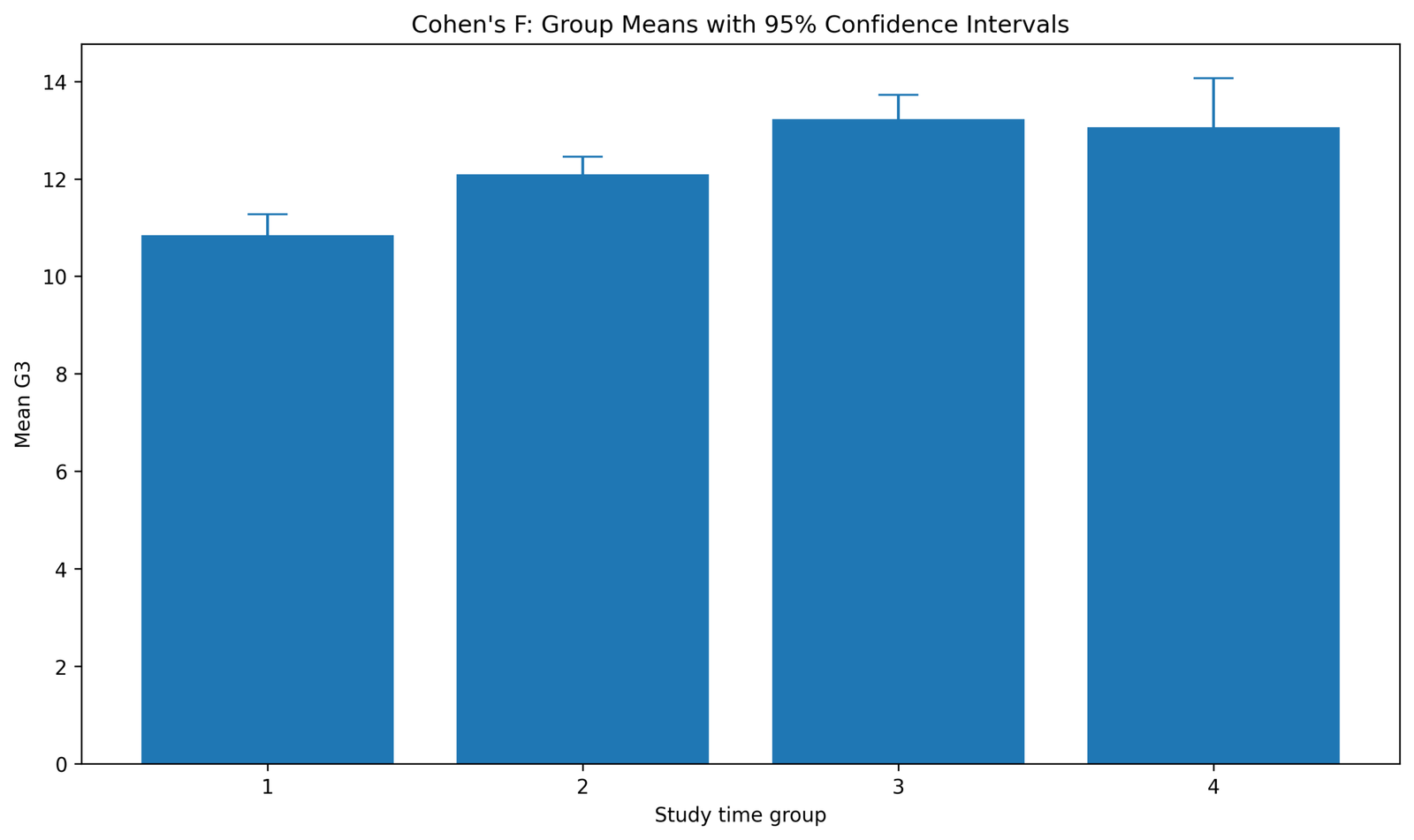
This chart shows the mean G3 score for each studytime group. Studytime group 1 has the lowest mean, group 2 is higher, group 3 has the highest mean, and group 4 remains close to group 3. The visible pattern shows that higher studytime groups generally have higher final grades.
The confidence intervals show uncertainty around each mean. The first three groups have comparatively tighter intervals, while group 4 has a wider interval. This wider interval means the group 4 mean is less precise, but it still stays in the higher G3 range.
This chart explains the practical direction behind Cohen’s f. Cohen’s f is not calculated from the bars directly, but the bars show why the ANOVA effect exists: the group means are not flat across studytime categories.
Python Chart 2: Cohen’s f Conversion Summary
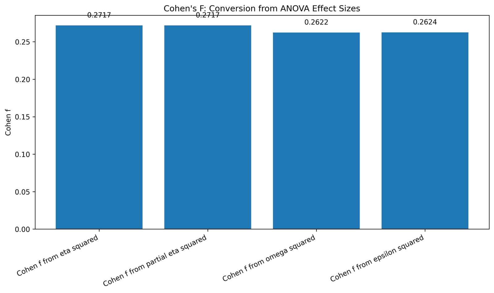
This chart shows how Cohen’s f changes depending on which ANOVA effect-size estimate is used. Cohen’s f from eta squared is 0.2717, and Cohen’s f from partial eta squared is also 0.2717. These two values match because this is a one-way ANOVA example where eta squared and partial eta squared are the same or nearly the same.
Cohen’s f from omega squared is 0.2622, and Cohen’s f from epsilon squared is 0.2624. These values are slightly lower because omega squared and epsilon squared are adjusted estimates of explained variance.
This chart is the main calculation evidence for the post. It shows that the effect remains in the same interpretation range even when the conversion is based on a more conservative adjusted effect-size value.
Python Chart 3: Effect Size Comparison
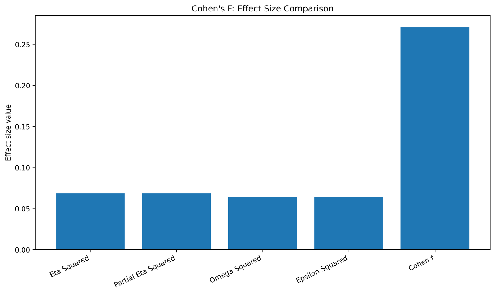
This chart compares the explained-variance effect sizes behind Cohen’s f. Eta squared and partial eta squared are the larger values, while omega squared and epsilon squared are slightly smaller. The small difference between the two pairs explains why the adjusted Cohen’s f values are slightly lower than the eta-based Cohen’s f value.
The chart supports a stable interpretation. The effect-size estimates are close enough that the practical conclusion does not change. Whether eta squared, partial eta squared, omega squared or epsilon squared is used, Cohen’s f remains around the medium range.
This chart should be read before the conversion summary when explaining the logic. Cohen’s f is a conversion, so the original explained-variance values determine the final Cohen’s f values.
Python Chart 4: ANOVA F Distribution Curve
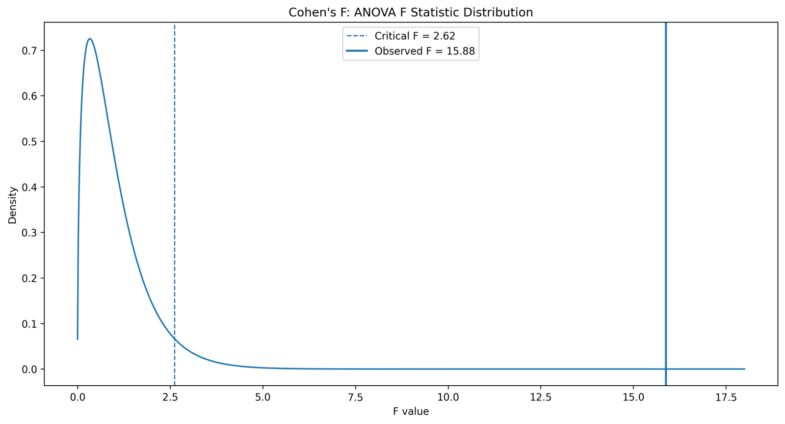
This chart shows the ANOVA F distribution for the studytime effect on G3. The critical F value is 2.62, and the observed F statistic is 15.88.
The observed F line is far to the right of the critical F line. This means the group mean difference is statistically significant. The studytime groups differ more than expected from random within-group variation.
This chart is important because it separates statistical significance from practical size. The ANOVA F statistic gives the significance decision, while Cohen’s f gives the standardized effect-size interpretation.
Python Chart 5: Variance Explained Pie Chart
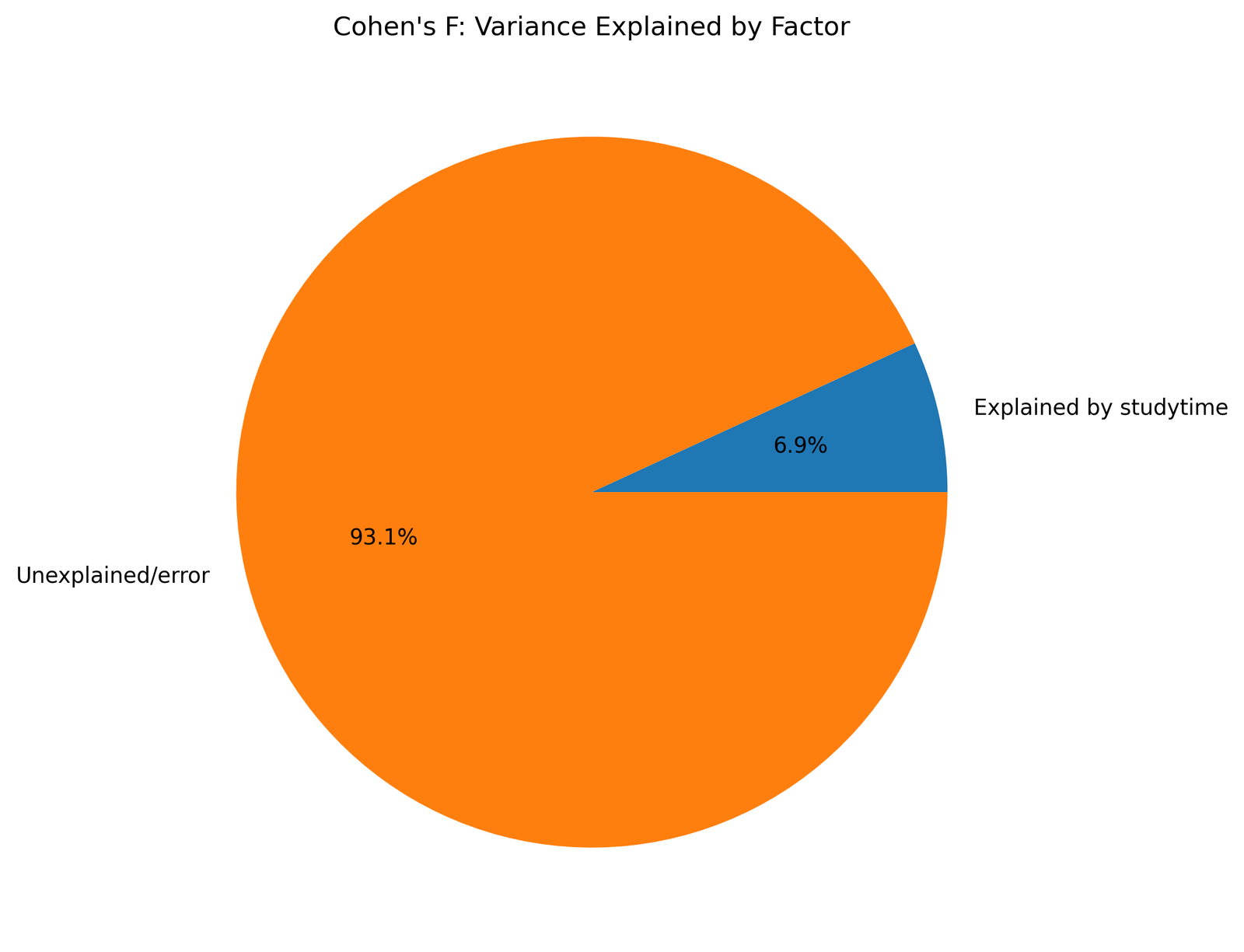
This pie chart shows the explained-variance meaning behind Cohen’s f. Studytime explains 6.9% of the variation in G3, while 93.1% remains unexplained or within-group variation.
The small explained slice does not mean the effect is useless. In educational data, final grades are influenced by many factors, so a single studytime factor explaining nearly seven percent of variation is still meaningful.
This chart connects eta squared to Cohen’s f. Eta squared expresses the result as percent variance explained, while Cohen’s f converts that same idea into a standardized effect-size scale used for interpretation and power analysis.
Python Chart 6: Boxplot of G3 by Studytime Group
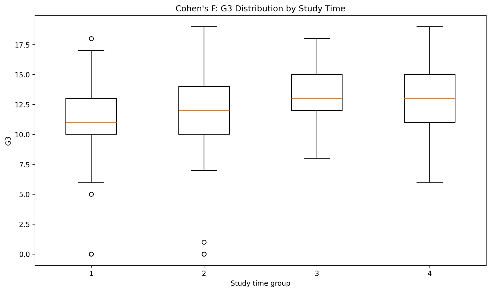
This boxplot shows the full G3 distribution inside each studytime group. The center of group 1 is lower than the centers of groups 3 and 4, while group 2 sits between the lower and higher groups. This distribution pattern supports the same direction shown in the group mean chart.
The groups overlap, and the lower studytime groups contain low outliers. This explains why Cohen’s f is medium rather than large. The group means differ, but individual scores still vary widely within each group.
For reporting, the boxplot gives the practical context behind the numeric effect size. Cohen’s f around 0.272 is medium because the group centers shift upward, but the distributions are not completely separated.
Python Chart 7: Cohen’s f Interpretation Thresholds
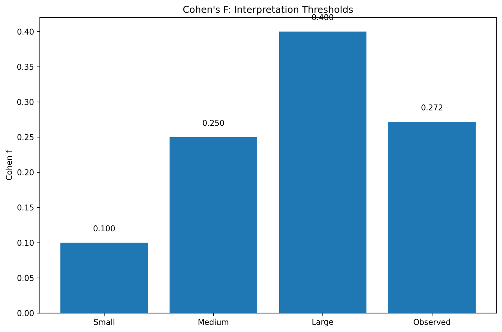
This chart compares the observed Cohen’s f value with common interpretation thresholds. The small threshold is 0.10, the medium threshold is 0.25, and the large threshold is 0.40. The observed value is shown as about 0.272.
The observed value is just above the medium threshold and clearly below the large threshold. This makes the final interpretation straightforward: the studytime effect on G3 is medium in size.
This chart should be used as the final practical summary. It translates the numeric value into a reporting category and prevents overstatement. The result is meaningful, but it should not be described as a large effect.
R Chart-by-Chart Validation
The R validation charts repeat the same Cohen’s f workflow in a second software environment. They confirm the same group mean direction, conversion values, effect-size comparison, ANOVA F decision, explained variance, group distribution and interpretation threshold.
R Chart 1: Group Means with 95% Confidence Intervals
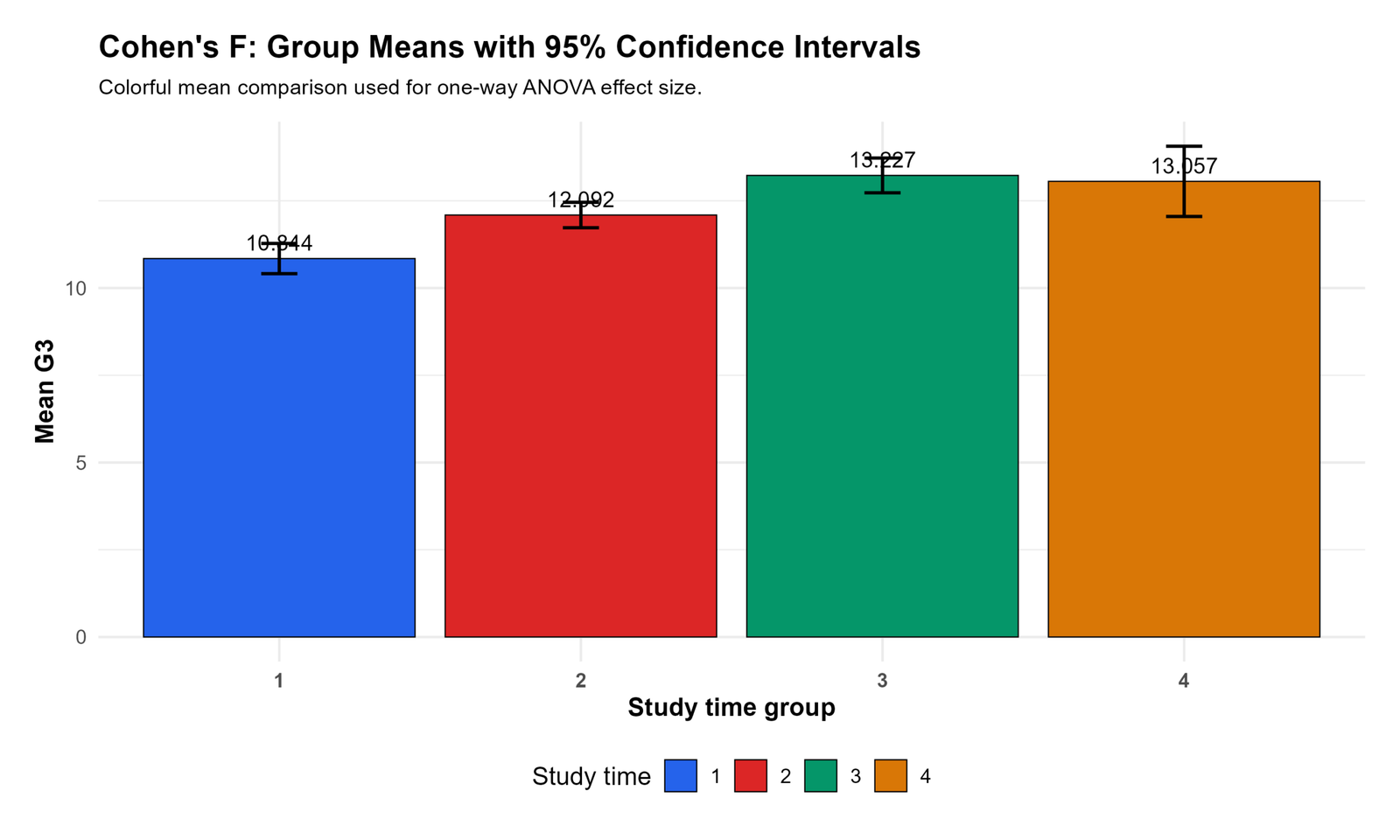
This R chart validates the same group mean pattern shown in Python. Studytime group 1 has the lowest mean G3, group 2 is higher, and groups 3 and 4 remain in the higher grade range.
The confidence intervals show the same precision pattern. Group 4 has the widest interval, while the larger groups have narrower intervals. This confirms that the direction of the effect is stable, but the fourth group is less precisely estimated.
In reporting, this chart confirms that the Cohen’s f calculation is based on a real group mean pattern. The practical effect size is supported by the visible increase in G3 across studytime groups.
R Chart 2: Cohen’s f Conversion Summary
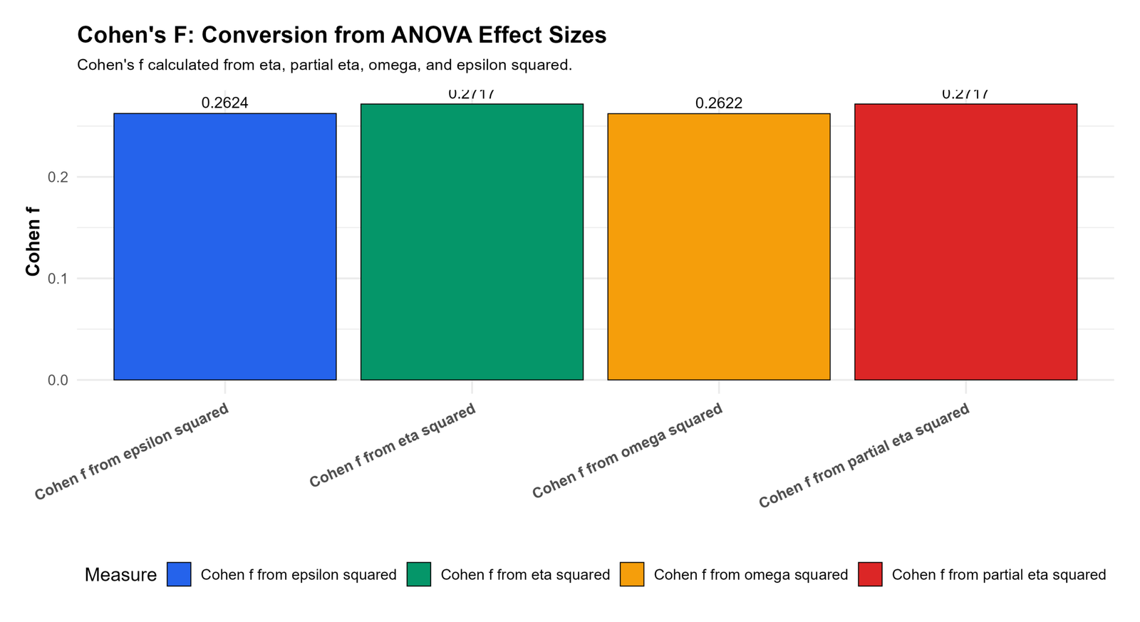
This R chart confirms the conversion values shown in Python. Cohen’s f from eta squared and partial eta squared is around 0.2717, while the conversions from omega squared and epsilon squared are around 0.2622 and 0.2624.
The adjusted conversions are slightly smaller because omega squared and epsilon squared reduce the explained-variance estimate. The difference is small, so the practical interpretation remains the same.
In the final report, this chart validates the conversion method. It shows that the medium-effect conclusion is not dependent on one software output or one effect-size formula.
R Chart 3: Effect Size Comparison
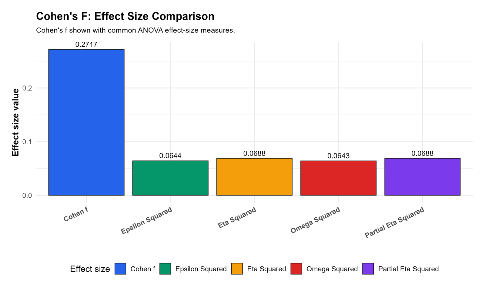
This chart confirms that eta squared and partial eta squared are the larger explained-variance estimates, while omega squared and epsilon squared are slightly smaller adjusted estimates.
The pattern is expected. Adjusted measures usually reduce the estimate slightly so the effect is not overstated. The values remain close enough that the interpretation stays medium.
In reporting, this R chart supports a careful effect-size statement. The result can be reported with Cohen’s f from eta squared, while also noting that adjusted conversions still support the same practical category.
R Chart 4: ANOVA F Distribution Curve
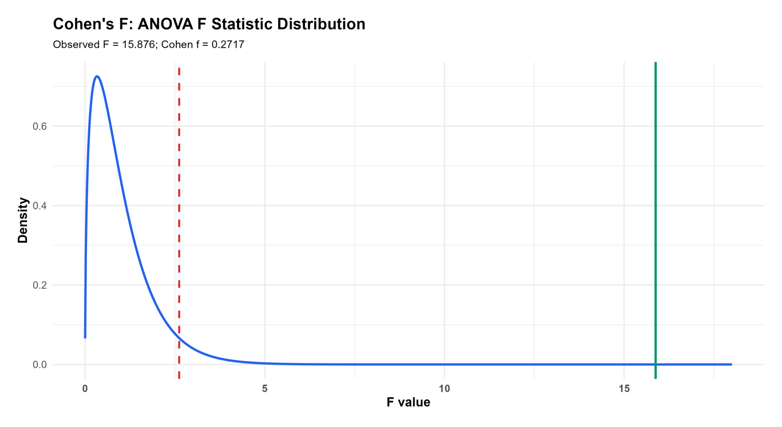
The R F distribution curve confirms the same significance decision. The observed F statistic is about 15.88, and the critical F value is about 2.62.
The observed F statistic is far beyond the critical value. This confirms that the studytime group means differ statistically in the ANOVA model.
In the final explanation, this chart should be linked to Cohen’s f. The ANOVA F statistic confirms significance, and Cohen’s f explains practical size.
R Chart 5: Variance Explained Pie Chart
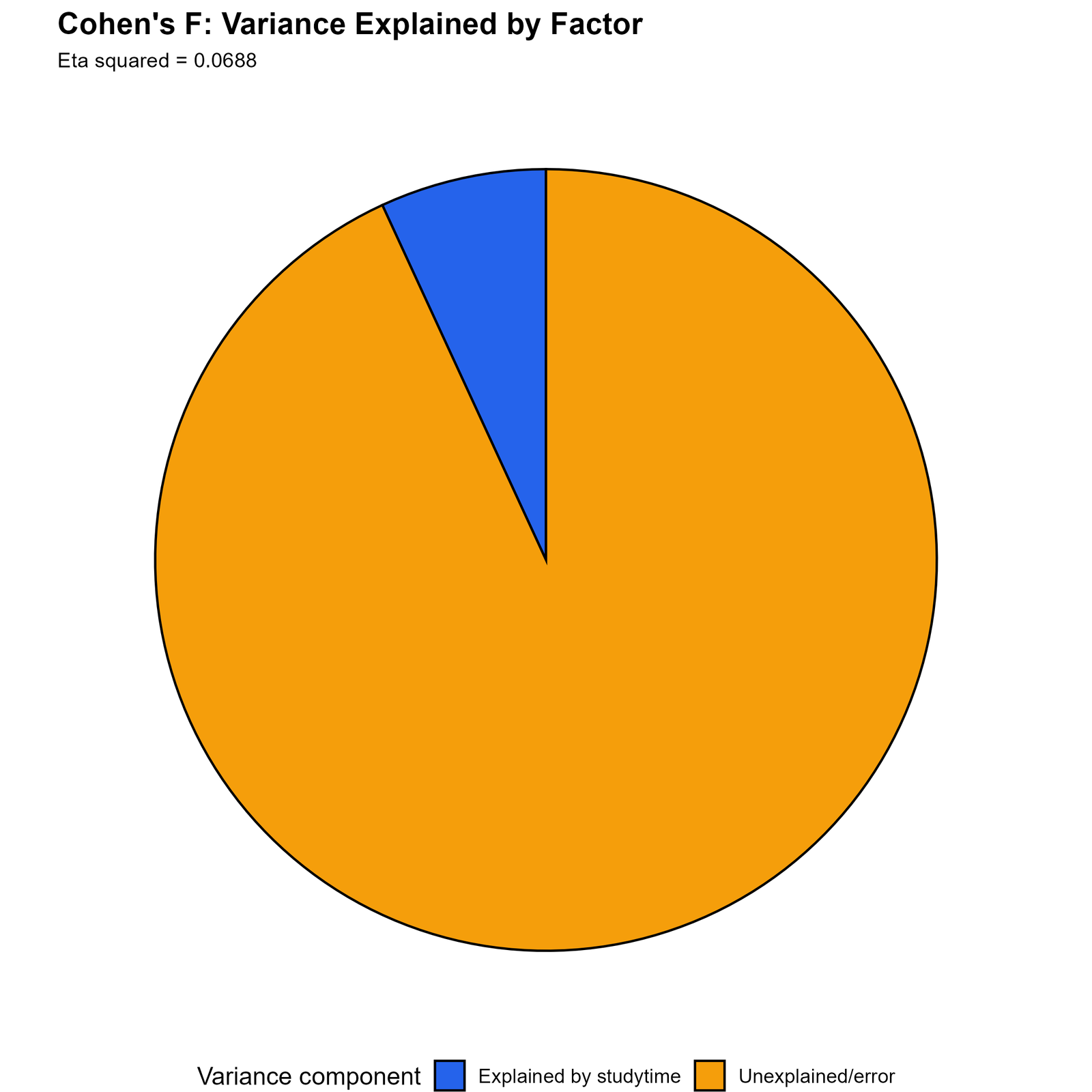
This R pie chart confirms that studytime explains about 6.9% of the variation in G3, while about 93.1% remains unexplained or within-group variation.
The chart makes the explained-variance base of Cohen’s f clear. Cohen’s f is not a separate descriptive statistic; it is calculated from the same explained-variance idea shown in this pie chart.
In reporting, this chart supports wording such as “studytime explained approximately 6.9% of the variation in G3, corresponding to Cohen’s f of about 0.272.”
R Chart 6: Boxplot of G3 by Studytime Group
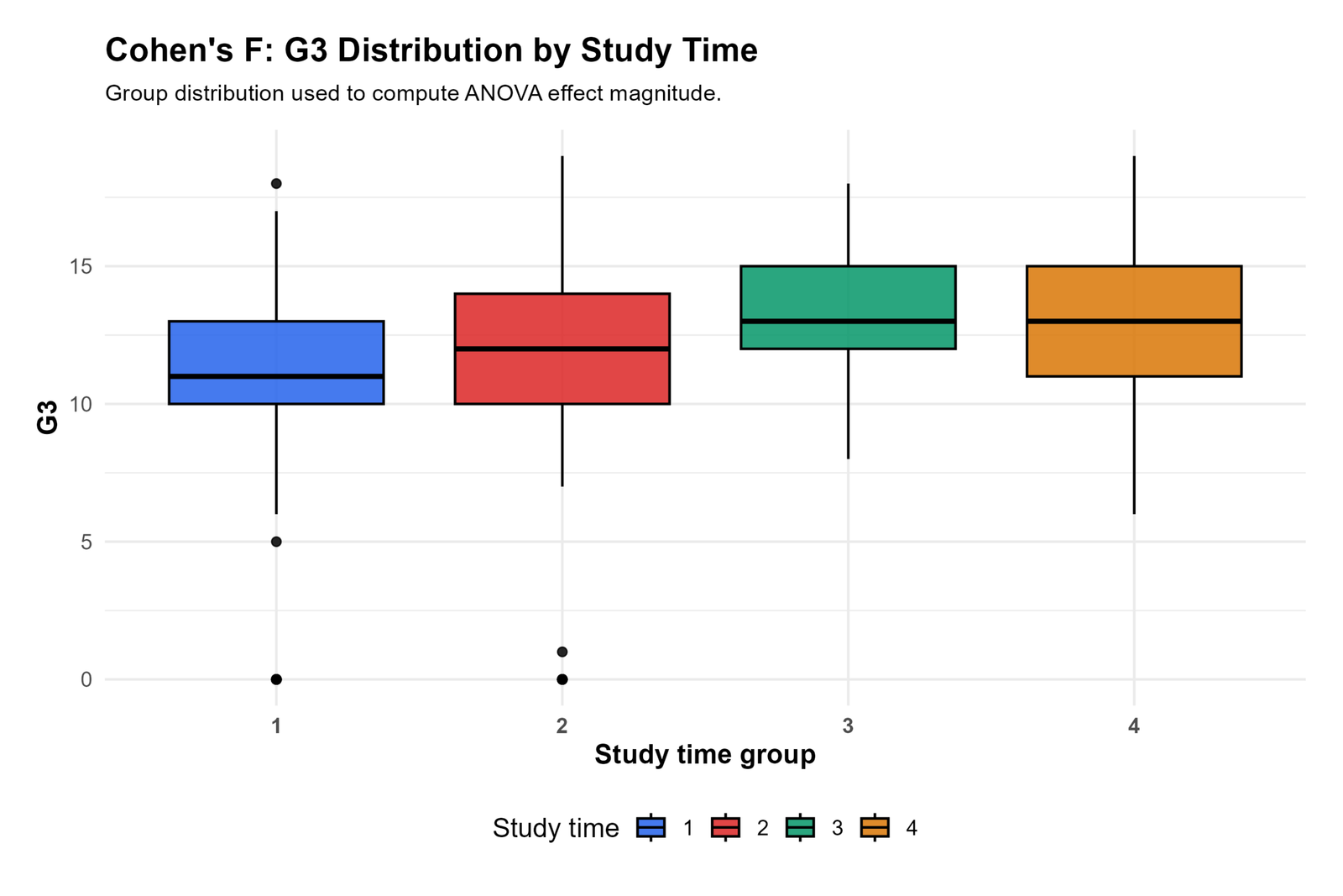
The R boxplot confirms the same group distribution pattern. Higher studytime groups have higher centers than the lowest studytime group, but the distributions still overlap.
The overlap explains why the effect is medium rather than large. A large effect would show stronger separation among group distributions, while this output shows a meaningful but still overlapping group pattern.
In the final article, this chart validates the practical interpretation. Cohen’s f around 0.272 is consistent with a visible group shift and continued within-group variation.
R Chart 7: Cohen’s f Interpretation Thresholds
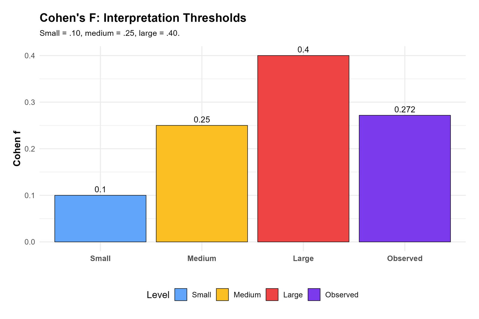
This R chart confirms the threshold interpretation. The small threshold is 0.10, the medium threshold is 0.25, the large threshold is 0.40, and the observed value is about 0.272.
The observed bar is above the medium threshold and below the large threshold. This validates the conclusion that the effect is medium.
In reporting, this chart should be used as the final visual conclusion. It gives readers a direct comparison between the observed Cohen’s f and the standard interpretation cutoffs.
SPSS Output Interpretation for Cohen’s F
The SPSS output PDF is included as the downloadable software output for the Cohen’s F workflow. SPSS commonly reports partial eta squared in GLM output. Cohen’s f is then calculated from partial eta squared using the conversion formula.
Download Cohen’s F SPSS Output PDF
SPSS Output Items to Read
| SPSS Output Item | What It Shows | How It Is Used | Reporting Meaning |
|---|---|---|---|
| Descriptives | Group means and standard deviations for G3 by studytime. | Shows the direction of the effect. | Report group means before effect size. |
| ANOVA table | F statistic, degrees of freedom and p value. | Tests whether group means differ. | Report statistical significance. |
| Partial eta squared | SPSS GLM effect-size output. | Used to calculate Cohen’s f. | Convert to f with √[η²/(1−η²)]. |
| Estimated marginal means | Mean pattern across groups. | Confirms the studytime direction. | Explains which groups are higher or lower. |
| Residual diagnostics | Model error pattern. | Checks ANOVA assumptions. | Discuss before final interpretation. |
| Cohen’s f calculation | Converted standardized effect size. | Used for interpretation and power analysis. | Report f ≈ 0.272, medium effect. |
SPSS Reporting Summary
The SPSS interpretation should first identify the ANOVA model, then read the effect-size output, then convert the effect-size value to Cohen’s f. In this example, the charted ANOVA result is significant and the explained variance is about 6.9%. Converting this effect-size estimate gives Cohen’s f around 0.272.
The correct SPSS-style conclusion is that studytime has a statistically significant and medium-sized effect on G3. Cohen’s f is useful because it turns the explained-variance result into a standardized effect-size value that can also be used in power analysis.
SPSS, R, Python and Excel Workflows for Cohen’s F
The same Cohen’s F workflow can be reproduced in SPSS, R, Python and Excel. The main steps are to run ANOVA, extract eta squared or partial eta squared, convert that value into Cohen’s f, and compare the result with interpretation thresholds.
SPSS Workflow
| Step | SPSS Menu or Syntax | Purpose |
|---|---|---|
| Open data | File > Open > Data | Load G3 and studytime variables. |
| Run GLM | Analyze > General Linear Model > Univariate | Get ANOVA and partial eta squared. |
| Request effect size | Options > Estimates of effect size | Display partial eta squared. |
| Convert to Cohen’s f | Use formula or compute variable | Calculate √[partial η²/(1−partial η²)]. |
| Interpret threshold | Compare with .10, .25 and .40 | Classify effect as small, medium or large. |
| Export output | OUTPUT EXPORT | Save SPSS output PDF. |
R Workflow
| Step | R Action | Purpose |
|---|---|---|
| Read data | read.csv("dataset.csv") | Load dataset. |
| Run ANOVA | aov(G3 ~ studytime, data=df) | Fit one-way ANOVA. |
| Extract sum of squares | summary(model) | Calculate eta squared. |
| Convert to Cohen’s f | sqrt(eta_sq/(1-eta_sq)) | Get standardized effect size. |
| Use effectsize package | effectsize | Calculate eta squared and related measures. |
| Interpret result | Compare with thresholds | Report medium effect if f is near .27. |
Python Workflow
| Step | Python Action | Purpose |
|---|---|---|
| Read data | pandas.read_csv() | Load dataset. |
| Fit ANOVA model | ols("G3 ~ C(studytime)") | Fit one-way ANOVA model. |
| Get ANOVA table | sm.stats.anova_lm() | Extract sum of squares and F statistic. |
| Calculate eta squared | ss_between / ss_total | Get explained variance. |
| Calculate Cohen’s f | np.sqrt(eta_sq/(1-eta_sq)) | Convert explained variance to f. |
| Create threshold chart | Bar chart | Compare observed f with small, medium and large values. |
Excel Workflow
| Excel Task | Formula or Tool | Purpose |
|---|---|---|
| Run ANOVA | Data Analysis ToolPak > ANOVA: Single Factor | Get sum of squares and F statistic. |
| Total sum of squares | =SS_Between + SS_Within | Calculate total variation. |
| Eta squared | =SS_Between / SS_Total | Calculate explained variance. |
| Cohen’s f | =SQRT(EtaSquared/(1-EtaSquared)) | Convert eta squared to Cohen’s f. |
| Threshold comparison | Small .10, medium .25, large .40 | Classify the effect size. |
| Variance explained | =EtaSquared*100 | Report percent variance explained. |
Code Blocks for Cohen’s F
SPSS Syntax for Cohen’s F Workflow
* Cohen's F workflow in SPSS.
* Dependent variable: G3.
* Factor: studytime.

TITLE "Cohen's F for ANOVA Effect Size: G3 by Studytime".

UNIANOVA G3 BY studytime
  /METHOD=SSTYPE(3)
  /INTERCEPT=INCLUDE
  /PRINT=DESCRIPTIVE ETASQ HOMOGENEITY
  /CRITERIA=ALPHA(.05)
  /DESIGN=studytime.

* Cohen's f is calculated from partial eta squared:
* f = SQRT(partial_eta_squared / (1 - partial_eta_squared)).

OUTPUT EXPORT
  /CONTENTS EXPORT=VISIBLE
  /PDF DOCUMENTFILE="Cohens-F-SPSS-Output.pdf".
Python Code for Cohen’s F
import pandas as pd
import numpy as np
import statsmodels.api as sm
from statsmodels.formula.api import ols

df = pd.read_csv("dataset.csv")

df["G3"] = pd.to_numeric(df["G3"], errors="coerce")
df["studytime"] = df["studytime"].astype("category")

df_model = df.dropna(subset=["G3", "studytime"]).copy()

model = ols("G3 ~ C(studytime)", data=df_model).fit()
anova_table = sm.stats.anova_lm(model, typ=2)

ss_between = anova_table.loc["C(studytime)", "sum_sq"]
df_between = anova_table.loc["C(studytime)", "df"]
ss_within = anova_table.loc["Residual", "sum_sq"]
df_within = anova_table.loc["Residual", "df"]

ss_total = ss_between + ss_within
ms_within = ss_within / df_within

eta_squared = ss_between / ss_total
partial_eta_squared = ss_between / (ss_between + ss_within)
omega_squared = (ss_between - df_between * ms_within) / (ss_total + ms_within)
epsilon_squared = (ss_between - df_between * ms_within) / ss_total

cohens_f_eta = np.sqrt(eta_squared / (1 - eta_squared))
cohens_f_partial_eta = np.sqrt(partial_eta_squared / (1 - partial_eta_squared))
cohens_f_omega = np.sqrt(omega_squared / (1 - omega_squared))
cohens_f_epsilon = np.sqrt(epsilon_squared / (1 - epsilon_squared))

print(anova_table)
print("Eta squared:", eta_squared)
print("Partial eta squared:", partial_eta_squared)
print("Omega squared:", omega_squared)
print("Epsilon squared:", epsilon_squared)
print("Cohen's f from eta squared:", cohens_f_eta)
print("Cohen's f from partial eta squared:", cohens_f_partial_eta)
print("Cohen's f from omega squared:", cohens_f_omega)
print("Cohen's f from epsilon squared:", cohens_f_epsilon)
R Code for Cohen’s F
df <- read.csv("dataset.csv")

df$G3 <- as.numeric(df$G3)
df$studytime <- as.factor(df$studytime)

df_model <- na.omit(df[, c("G3", "studytime")])

model <- aov(G3 ~ studytime, data = df_model)
summary(model)

anova_table <- summary(model)[[1]]

ss_between <- anova_table["studytime", "Sum Sq"]
df_between <- anova_table["studytime", "Df"]
ss_within <- anova_table["Residuals", "Sum Sq"]
df_within <- anova_table["Residuals", "Df"]

ss_total <- ss_between + ss_within
ms_within <- ss_within / df_within

eta_squared <- ss_between / ss_total
partial_eta_squared <- ss_between / (ss_between + ss_within)
omega_squared <- (ss_between - df_between * ms_within) / (ss_total + ms_within)
epsilon_squared <- (ss_between - df_between * ms_within) / ss_total

cohens_f_eta <- sqrt(eta_squared / (1 - eta_squared))
cohens_f_partial_eta <- sqrt(partial_eta_squared / (1 - partial_eta_squared))
cohens_f_omega <- sqrt(omega_squared / (1 - omega_squared))
cohens_f_epsilon <- sqrt(epsilon_squared / (1 - epsilon_squared))

data.frame(
  eta_squared = eta_squared,
  partial_eta_squared = partial_eta_squared,
  omega_squared = omega_squared,
  epsilon_squared = epsilon_squared,
  cohens_f_eta = cohens_f_eta,
  cohens_f_partial_eta = cohens_f_partial_eta,
  cohens_f_omega = cohens_f_omega,
  cohens_f_epsilon = cohens_f_epsilon
)
Excel Formulas for Cohen’s F
Run ANOVA:
Data > Data Analysis > ANOVA: Single Factor

Total sum of squares:
=SS_Between + SS_Within

Eta squared:
=SS_Between / SS_Total

Partial eta squared:
=SS_Between / (SS_Between + SS_Within)

Omega squared:
=(SS_Between - df_Between * MS_Within) / (SS_Total + MS_Within)

Epsilon squared:
=(SS_Between - df_Between * MS_Within) / SS_Total

Cohen's f from eta squared:
=SQRT(EtaSquared / (1 - EtaSquared))

Cohen's f from partial eta squared:
=SQRT(PartialEtaSquared / (1 - PartialEtaSquared))

Cohen's f from omega squared:
=SQRT(OmegaSquared / (1 - OmegaSquared))

Cohen's f from epsilon squared:
=SQRT(EpsilonSquared / (1 - EpsilonSquared))

Interpretation:
0.10 = small
0.25 = medium
0.40 = large
APA Reporting Wording
When reporting Cohen’s F, include the ANOVA result and then report Cohen’s f as the practical effect-size measure. Do not report Cohen’s f alone without explaining the ANOVA model and the factor being tested.
APA-style report: A one-way ANOVA was used to compare G3 final grade across four studytime groups. The ANOVA result was statistically significant, F(3, 645) ≈ 15.88, p < .001. Studytime explained approximately 6.9% of the variance in G3. Converting eta squared to Cohen’s f produced f = 0.2717, which is above the medium threshold of 0.25 and below the large threshold of 0.40. The studytime effect was therefore interpreted as medium in practical size.
Short reporting version: The studytime effect on G3 was statistically significant and medium in size, F(3, 645) ≈ 15.88, p < .001, Cohen’s f ≈ 0.272.
Common Mistakes
| Mistake | Why It Is Wrong | Correct Practice |
|---|---|---|
| Confusing Cohen’s f with the ANOVA F statistic | The ANOVA F statistic tests significance, while Cohen’s f measures effect size. | Report both separately. |
| Reporting only p value | The p value does not show practical magnitude. | Report Cohen’s f, eta squared or another effect-size measure. |
| Calling 0.272 a large effect | It is above 0.25 but below 0.40. | Report it as medium. |
| Using adjusted and unadjusted conversions without explanation | Omega squared and epsilon squared produce slightly lower f values. | State which source effect-size measure was used. |
| Ignoring variance explained | Cohen’s f comes from explained variance. | Also explain that studytime explains about 6.9% of G3 variation. |
| Using Cohen’s f without assumption checks | Effect size still comes from the fitted ANOVA model. | Review ANOVA Assumptions, Levene Test, Q-Q Plot Normality Check, P-P Plot Normality Check and Outlier Detection. |
When to Use Cohen’s F
Use Cohen’s f when reporting ANOVA-family effect sizes or planning sample size and power for ANOVA designs. It is especially useful when the same effect must be compared across different ANOVA models or entered into a power-analysis tool.
| Situation | Use Cohen’s f? | Reporting Note |
|---|---|---|
| One-way ANOVA | Yes | Convert eta squared or partial eta squared to Cohen’s f. |
| ANCOVA | Yes | Use partial eta squared from the adjusted model. |
| Power analysis | Yes | Cohen’s f is commonly used for ANOVA sample-size planning. |
| Regression-only model | Sometimes | Use f² when reporting regression-style local effect size. |
| Simple two-group mean comparison | Usually no | Use Cohen’s d or a t-test effect size instead. |
For related mean-comparison and effect-size guides, see ANOVA Effect Size, ANOVA in SPSS, ANOVA in Python, ANOVA in R, ANOVA Assumptions, ANCOVA, Balanced ANOVA, Brown Forsythe ANOVA, Brown-Forsythe Test, T Test vs ANOVA and Statistical Power.
Downloads and Resources for Cohen’s F
The verified SPSS output PDF below documents the worked example. The complete Python, R and Excel calculations are included in the article.
FAQs About Cohen’s F
What is Cohen’s F?
Cohen’s f is a standardized ANOVA effect-size measure. It converts explained variance into a value that can be interpreted as small, medium or large.
What is Cohen’s f used for?
Cohen’s f is used to report ANOVA-family effect size and to plan sample size or statistical power for ANOVA designs.
What is the formula for Cohen’s f?
The common formula is f = square root of eta squared divided by one minus eta squared.
What was Cohen’s f in this example?
Cohen’s f was about 0.2717 from eta squared and partial eta squared. The threshold chart displays the observed value as about 0.272.
Is Cohen’s f of 0.272 small, medium or large?
Cohen’s f of 0.272 is interpreted as medium because it is above 0.25 and below 0.40.
What is the difference between Cohen’s f and the ANOVA F statistic?
The ANOVA F statistic tests whether group means differ statistically. Cohen’s f measures the practical size of the group effect.
How do I calculate Cohen’s f from eta squared?
Use f = SQRT(eta squared / (1 – eta squared)). In this example, eta squared around .069 gives Cohen’s f around .272.
How much variance was explained in this Cohen’s f example?
Studytime explained about 6.9% of the variation in G3, while about 93.1% remained unexplained or within-group variation.
Can SPSS calculate Cohen’s f directly?
SPSS often reports partial eta squared in GLM output. Cohen’s f can be calculated from partial eta squared using the conversion formula.
How do I report Cohen’s f in APA style?
A concise report is: The studytime effect on G3 was statistically significant and medium in size, F(3, 645) ≈ 15.88, p < .001, Cohen’s f ≈ 0.272.

