
F-value, critical value, p-value and reporting
F Distribution: F-Value Interpretation & ANOVA Report
The F distribution turns an ANOVA F-value into a right-tail p-value using numerator and denominator degrees of freedom. Learn how to compare observed and critical F, interpret significance, and write a clear ANOVA report.
Quick Answer: F Distribution Result
The worked F Distribution example uses an ANOVA model where studytime is tested as a grouping factor for G3 final grade. The charted ANOVA result shows observed F = 15.876 and critical F = 2.619. The observed F line is far to the right of the critical F line, so the group mean difference is statistically significant.
The mean-square chart shows exactly where the F statistic comes from. The between-group mean square is 155.026, and the within-group mean square is 9.765. Dividing 155.026 by 9.765 gives an F statistic of about 15.876. This means between-group variation is much larger than the typical within-group variation.
Final interpretation: The observed ANOVA F statistic is far larger than the critical F value. The right-tail p-value area is extremely small on the chart, so the studytime group means differ statistically. The F statistic is large because the between-group mean square is much larger than the within-group mean square.
Important reporting point: The F distribution is always interpreted with two degrees of freedom: numerator degrees of freedom, usually called df1, and denominator degrees of freedom, usually called df2. The critical F value changes when alpha, df1 or df2 changes.
Table of Contents
- What Is the F Distribution?
- F Distribution Formula and ANOVA F Statistic
- Null and Alternative Hypothesis
- Dataset and Variables Used
- Python Chart-by-Chart Interpretation
- R Chart-by-Chart Validation
- SPSS Output Interpretation
- SPSS, R, Python and Excel Workflows
- Code Blocks for F Distribution
- APA Reporting Wording
- Common Mistakes
- When to Use F Distribution
- Downloads and Resources
- Related Guides
- FAQs
What Is the F Distribution?
The F Distribution is a right-skewed probability distribution used when a test statistic is built from a ratio of two variance estimates. In ANOVA, the F statistic compares variation between groups with variation inside groups. If the between-group variation is much larger than the within-group variation, the F statistic becomes large.
The F distribution is not one single curve. Its shape changes depending on two degrees of freedom values. The first degrees of freedom value, df1, is linked to the numerator of the F statistic. The second degrees of freedom value, df2, is linked to the denominator. That is why the same observed F value can have a different p value under different df1 and df2 combinations.
In this worked example, the observed ANOVA F statistic is 15.876 and the critical F value is 2.619. The observed F is far beyond the rejection boundary, so the F distribution supports a statistically significant ANOVA result for the studytime effect on G3.
Simple definition: The F distribution is used to decide whether a ratio of variances is large enough to be statistically significant. In ANOVA, that ratio is MS Between divided by MS Within.
The F distribution should be interpreted together with ANOVA in Python, ANOVA in R, ANOVA in SPSS, ANOVA Assumptions, ANOVA Effect Size, P Value, Null and Alternative Hypothesis, and Effect Size.
F Distribution Formula and ANOVA F Statistic
In one-way ANOVA, the F statistic is calculated by dividing the between-group mean square by the within-group mean square.
In the supplied mean-square chart, MS Between = 155.026 and MS Within = 9.765. Dividing those values gives the observed ANOVA F statistic.
This ratio is large because the variation between studytime group means is much larger than the typical variation remaining inside the groups. The F distribution then tells whether a ratio this large is unusual under the null hypothesis.
Critical F Value
The observed F statistic is 15.876, and the critical value at the displayed .05 level is 2.619. Since 15.876 is greater than 2.619, the result is statistically significant.
Right-Tail P-Value Area
The right-tail p-value area is the area under the F distribution curve to the right of the observed F statistic. In the supplied chart, the observed F line is far to the right, so the remaining right-tail area is visually tiny.
| F Distribution Item | Value in This Output | Meaning | Interpretation |
|---|---|---|---|
| MS Between | 155.026 | Variation explained by studytime groups. | Large compared with within-group mean square. |
| MS Within | 9.765 | Variation left inside groups. | Much smaller than MS Between. |
| Observed F | 15.876 | Ratio of MS Between to MS Within. | Large ANOVA test statistic. |
| Critical F at .05 | 2.619 | Decision boundary. | Observed F is far beyond the boundary. |
| Right-tail area | Very small in the chart | P-value region beyond observed F. | Supports rejecting the null hypothesis. |
Null and Alternative Hypothesis
For the ANOVA example shown in the F distribution charts, the null hypothesis says that the mean G3 score is the same across all studytime groups. The alternative hypothesis says that at least one studytime group mean differs.
| Hypothesis | Statement | Meaning in This Example | Decision Evidence |
|---|---|---|---|
| Null hypothesis | All group means are equal. | Studytime groups have the same mean G3. | Rejected because observed F is far above critical F. |
| Alternative hypothesis | At least one group mean differs. | At least one studytime group has a different mean G3. | Supported by observed F = 15.876. |
| Decision boundary | Critical F = 2.619 | F values beyond this point fall in the rejection region. | Observed F is beyond the boundary. |
| P-value area | Right tail beyond observed F | Area is visually very small. | Result is statistically significant. |
Decision for this example: Reject the null hypothesis. The observed F statistic is much larger than the critical F value, which means the studytime group means are not all equal in the ANOVA model.
Dataset and Variables Used
The worked example uses a student performance dataset. The dependent variable is G3 final grade, and the grouping factor is studytime. The F distribution is used after the ANOVA model calculates the between-group and within-group mean squares.
| Variable or Output | Role | Why It Matters for F Distribution | Where It Appears |
|---|---|---|---|
| G3 | Dependent variable | Final grade outcome being compared. | ANOVA model and mean squares. |
| studytime | Grouping factor | Defines the groups being compared. | Between-group mean square. |
| MS Between | Numerator mean square | Explained group variation. | Mean-square calculation chart. |
| MS Within | Denominator mean square | Unexplained within-group variation. | Mean-square calculation chart. |
| df1 | Numerator degrees of freedom | Changes the F distribution shape and critical values. | Density curves and df1 critical-value chart. |
| df2 | Denominator degrees of freedom | Changes the right-tail cutoff and p-value area. | Density curves and df2 critical-value chart. |
For supporting concepts, review Descriptive Statistics, Variance, Standard Deviation, Standard Error, Confidence Interval, Effect Size, Statistical Power, Type I and Type II Error and P Value.
Python Chart-by-Chart Interpretation
The Python charts below show the first F distribution workflow. They explain how F curves change by degrees of freedom, how the observed ANOVA F statistic is judged, how the right-tail p-value area works, how alpha changes the critical F value, and how mean squares produce the final F statistic.
Python Chart 1: F Distribution Curves by Degrees of Freedom
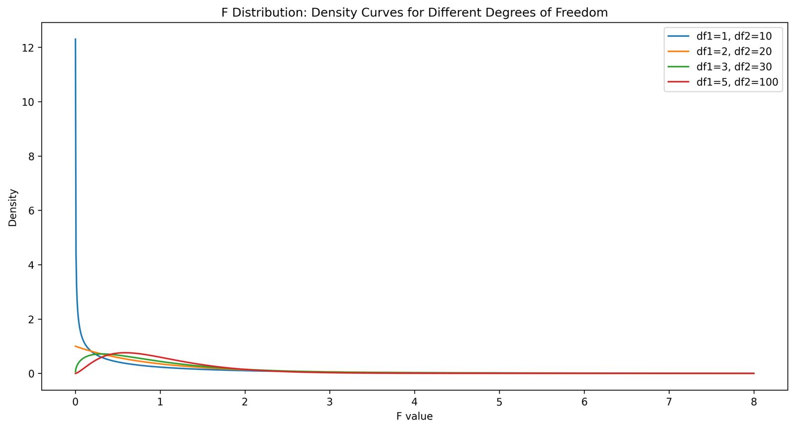
This chart compares several F distribution curves. The curve with df1 = 1 and df2 = 10 is sharply concentrated near zero and has a steep early drop. The curves with larger degrees of freedom become smoother and less extreme near zero.
The chart shows that the F distribution is always right-skewed and starts at nonnegative F values. An F statistic cannot be negative because it is a ratio of mean squares or variance estimates.
This chart explains why df1 and df2 matter. The same F statistic is judged against a different curve when the numerator and denominator degrees of freedom change.
Python Chart 2: Observed ANOVA F Distribution
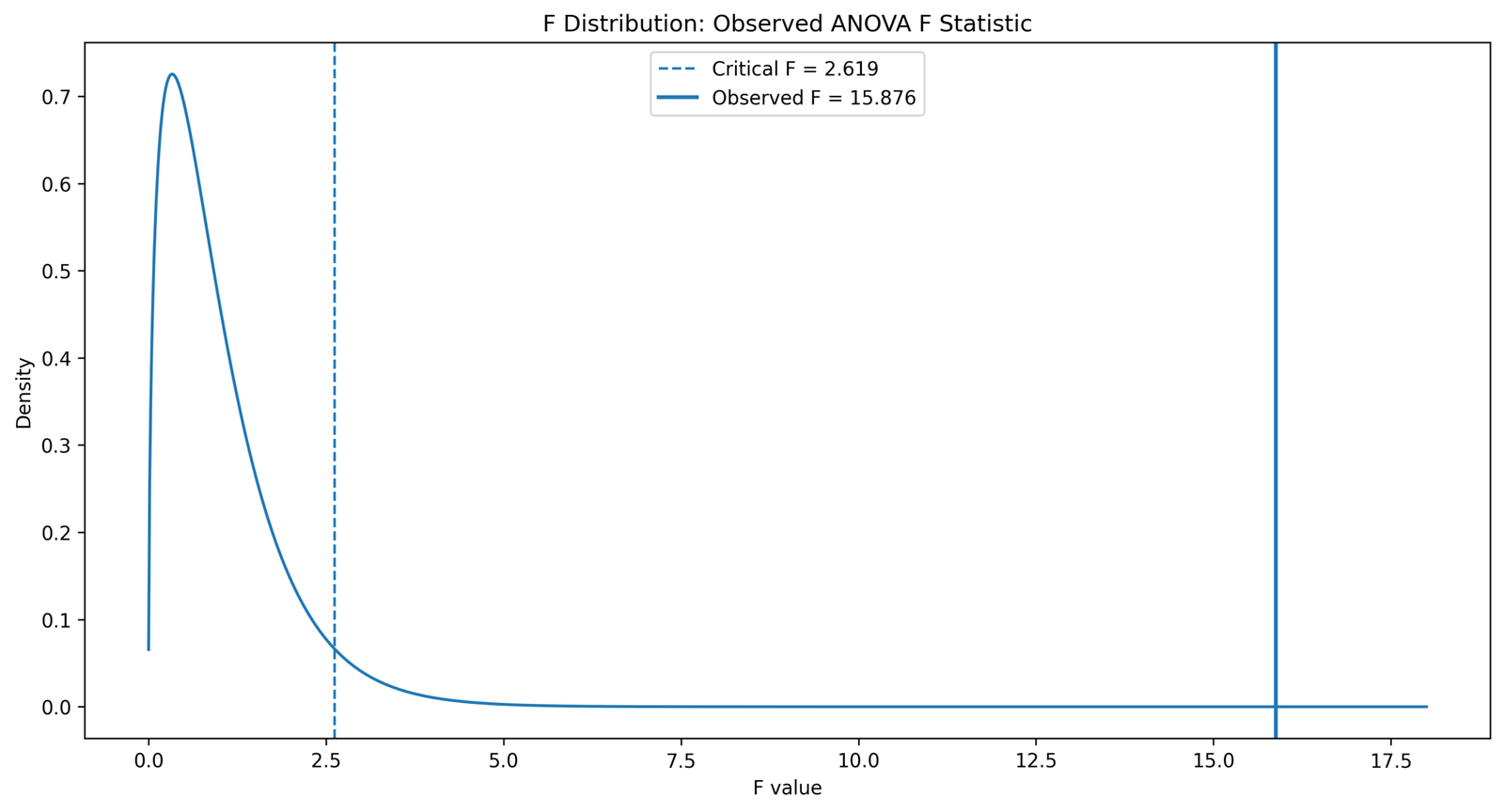
This chart shows the ANOVA F distribution with two vertical decision lines. The dashed critical F line is at 2.619, and the observed F line is at 15.876.
The observed F statistic is far to the right of the critical value. This means the observed ratio of mean squares is much larger than the cutoff needed for statistical significance at the displayed decision level.
This chart gives the central decision for the ANOVA example. Since the observed F statistic is far beyond the critical F line, the null hypothesis of equal group means is rejected.
Python Chart 3: Right-Tail P-Value Area
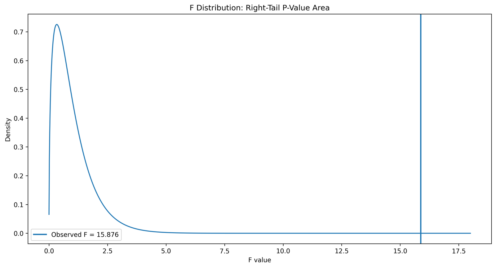
This chart shows how the p value is located in an F test. The observed F statistic is placed far to the right on the horizontal axis, so the p-value area is the small remaining area to the right of that vertical line.
The right-tail area is visually tiny because the observed F value is much larger than the values where the density curve is concentrated. Most of the F distribution curve is near smaller F values.
This chart should be used to explain why ANOVA p values are right-tail probabilities. A large F statistic is evidence against the null hypothesis because it leaves very little probability in the right tail under the null distribution.
Python Chart 4: Critical F Values by Alpha
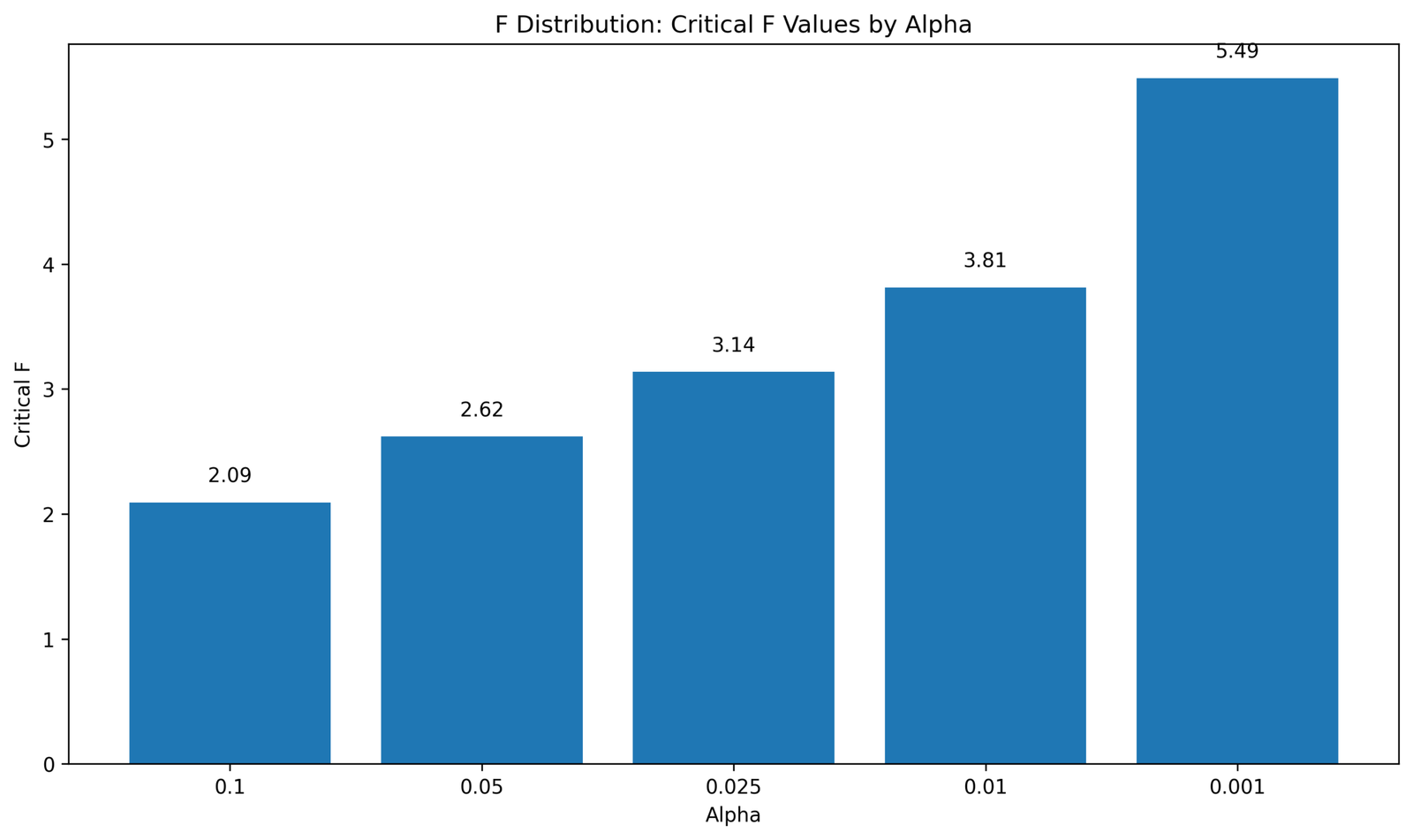
This chart shows how the critical F value changes when alpha changes. At alpha 0.10, the critical F value is 2.09. At alpha 0.05, it rises to 2.62. At alpha 0.025, it rises to 3.14. At alpha 0.01, it is 3.81, and at alpha 0.001, it is 5.49.
The pattern is clear: stricter alpha levels require larger F statistics before rejecting the null hypothesis. A smaller alpha leaves a smaller right-tail rejection area, so the cutoff moves farther to the right.
This chart is useful when explaining why the significance level must be selected before interpreting the test. The same observed F statistic is compared against a different critical value when alpha changes.
Python Chart 5: Critical F Changes as df1 Changes
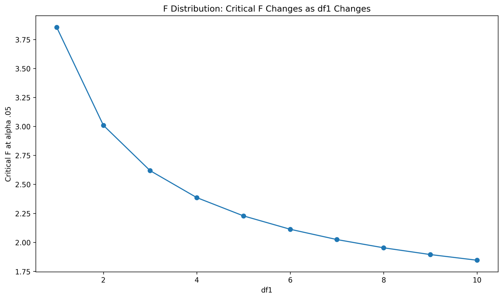
This chart shows the critical F value at alpha .05 as df1 changes. The critical value is highest when df1 is small and then gradually decreases as df1 increases.
The curve falls quickly from the first few df1 values and then flattens. By df1 values near 8, 9 and 10, the critical F values are much closer together than they are at the beginning of the curve.
This chart explains why degrees of freedom cannot be ignored. When the numerator degrees of freedom change, the rejection boundary changes even if alpha stays at .05.
Python Chart 6: Critical F Changes as df2 Changes
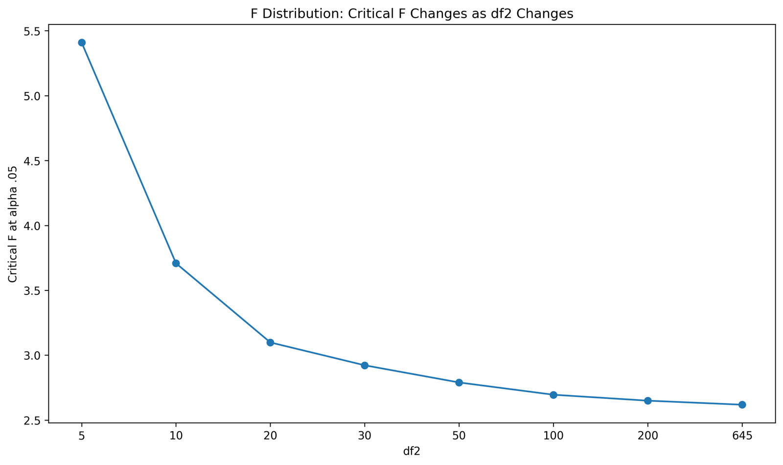
This chart shows the critical F value at alpha .05 as df2 changes. The critical F value is high when df2 is small, then drops as df2 increases. The chart moves from a high value near df2 = 5 down toward about 2.62 when df2 reaches 645.
The largest decrease occurs at the smaller df2 values. After df2 becomes large, the curve flattens and the critical F values change only slightly.
This chart is important for ANOVA because df2 usually represents within-group or error degrees of freedom. Larger denominator degrees of freedom give a more stable estimate of within-group variation and change the F cutoff.
Python Chart 7: Mean Squares Used to Calculate F
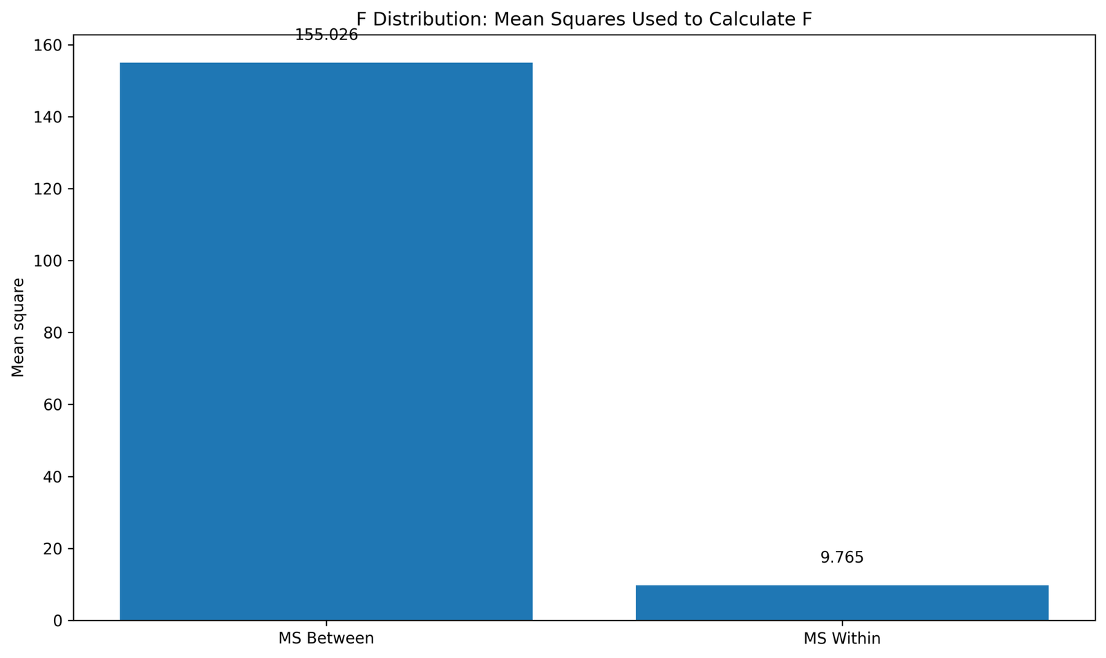
This chart shows the two mean squares used to calculate the ANOVA F statistic. MS Between is 155.026, while MS Within is 9.765.
The between-group mean square is much larger than the within-group mean square. This means the studytime group means vary much more than the typical variation left inside the groups.
This chart gives the calculation behind the F distribution decision. Dividing 155.026 by 9.765 gives an F statistic of about 15.876, which is the same observed F value shown in the distribution charts.
R Chart-by-Chart Validation
The R validation charts repeat the same F distribution workflow in a second software environment. They confirm the same density-curve behavior, observed F decision, p-value area, alpha critical values, df1 and df2 critical-value patterns, and mean-square calculation.
R Chart 1: F Distribution Curves by Degrees of Freedom
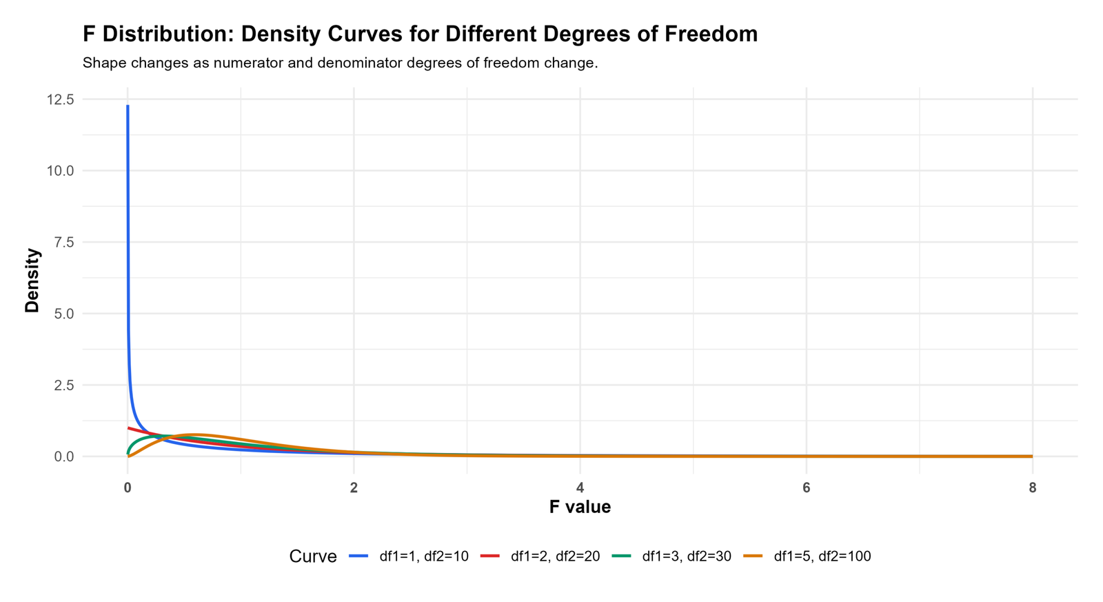
This R chart confirms that the shape of the F distribution changes with df1 and df2. The curve with smaller degrees of freedom is sharper near zero, while curves with larger degrees of freedom spread more smoothly.
The distribution remains nonnegative and right-skewed in every curve. This matches the definition of the F statistic as a ratio of nonnegative variance estimates.
In reporting, this chart validates the concept that F distribution interpretation depends on degrees of freedom, not only on the observed F statistic.
R Chart 2: Observed ANOVA F Distribution
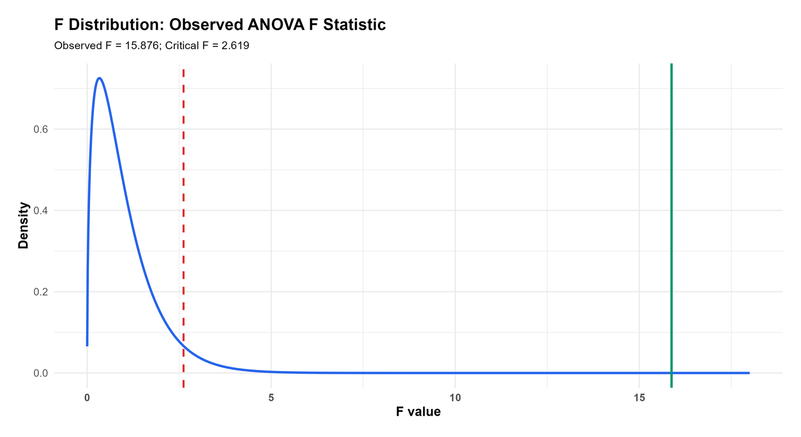
This R chart confirms the same ANOVA decision as Python. The critical F line is at 2.619, and the observed F line is at 15.876.
The observed F statistic is far beyond the critical boundary. This confirms that the studytime group effect is statistically significant in the F-test decision.
In the final article, this chart validates that the ANOVA decision is stable across software. Both Python and R show the observed statistic far into the right-tail rejection region.
R Chart 3: Right-Tail P-Value Area
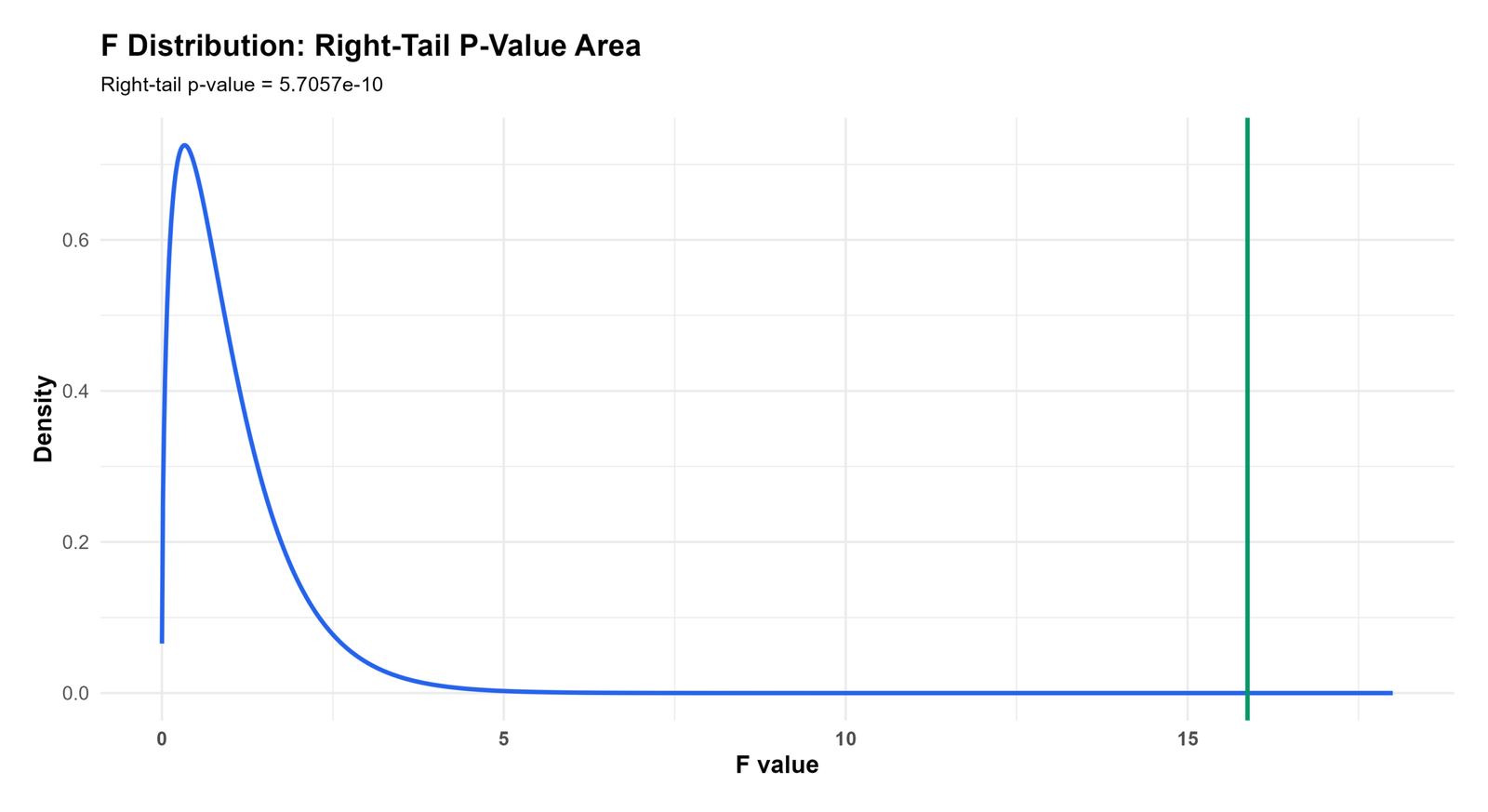
This R chart confirms that the p value for an F test is found in the right tail. The observed F statistic is so far to the right that the remaining tail area is visually very small.
The chart supports the same ANOVA conclusion as the observed-F distribution chart. A very large F statistic leaves very little probability beyond it under the null distribution.
In reporting, this chart should be used to explain the logic behind the p value. It shows why the ANOVA result is statistically significant without relying only on a table.
R Chart 4: Critical F Values by Alpha
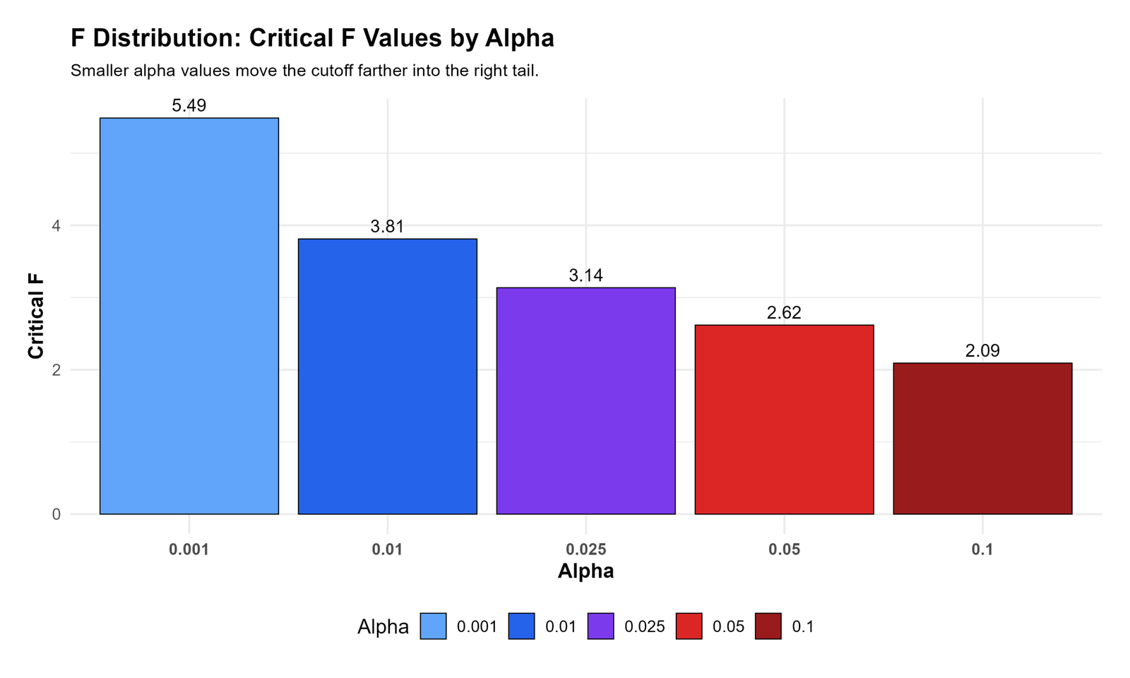
This R chart confirms the same alpha pattern. The critical F value increases as alpha becomes stricter. The bars move from 2.09 at alpha .10 to 5.49 at alpha .001.
The chart explains why a stricter significance level requires stronger evidence. When alpha becomes smaller, the rejection region moves farther into the right tail.
In reporting, this chart validates that the selected alpha level directly changes the critical value used for the F-test decision.
R Chart 5: Critical F Changes as df1 Changes
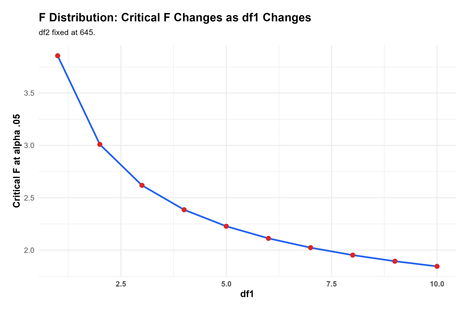
This R chart confirms that the critical F value decreases as df1 increases. The steepest decline appears at the smaller df1 values, and the line flattens at larger df1 values.
The chart shows that numerator degrees of freedom affect the right-tail cutoff. A test with df1 = 1 uses a different critical boundary from a test with df1 = 10.
In reporting, this chart supports a clear instruction: always report the degrees of freedom with an F statistic because the degrees of freedom determine the reference distribution.
R Chart 6: Critical F Changes as df2 Changes
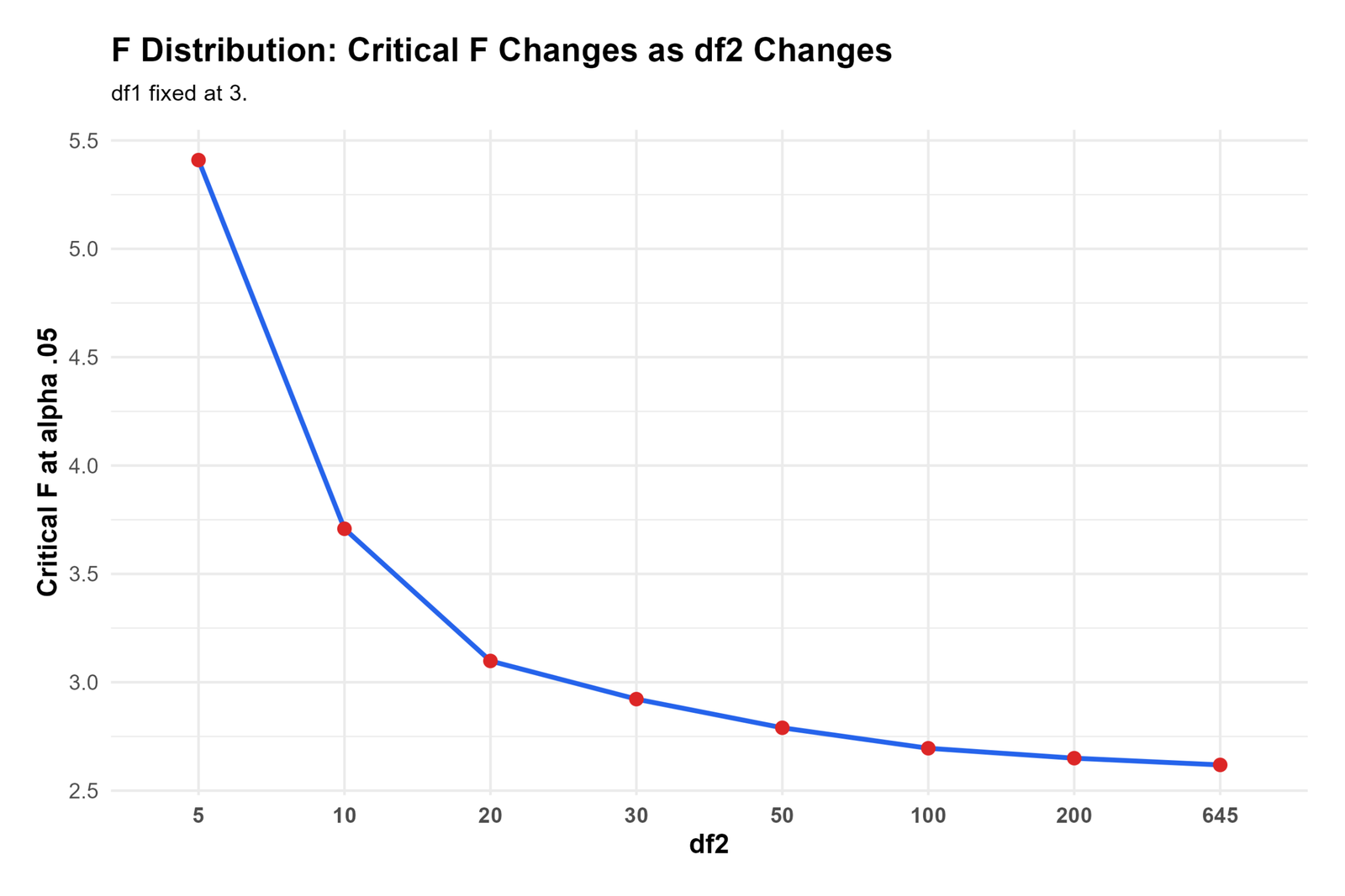
This R chart confirms that critical F decreases as df2 increases. The line drops strongly from small df2 values and then becomes nearly flat as df2 becomes large.
The final point near df2 = 645 is close to the same critical value used in the observed ANOVA F chart. This connects the degrees-of-freedom chart with the actual ANOVA decision.
In the final explanation, this chart should be used to show that a large error degrees of freedom value stabilizes the denominator side of the F distribution.
R Chart 7: Mean Squares Used to Calculate F
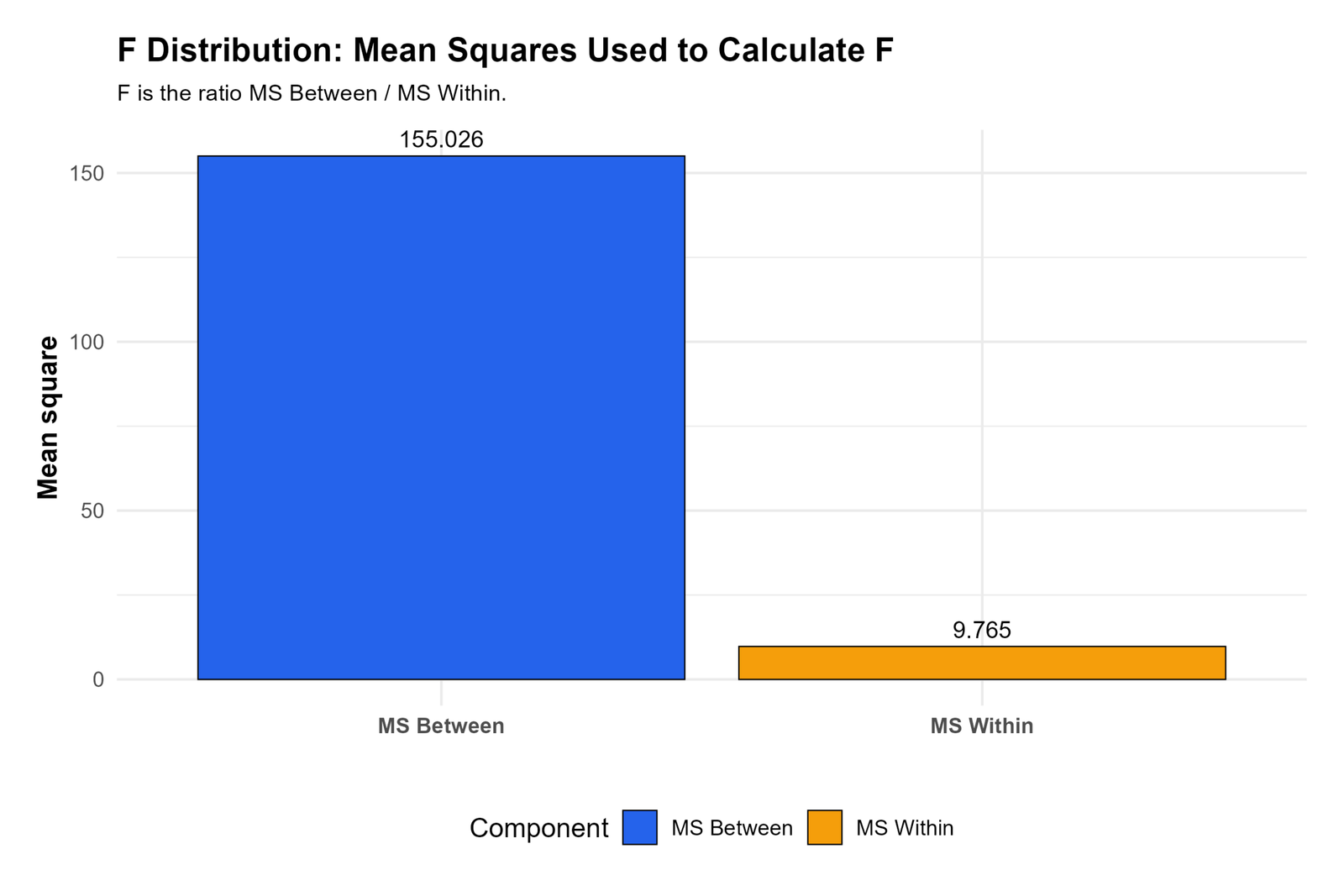
This R chart confirms the same mean-square calculation. MS Between is 155.026, and MS Within is 9.765.
The large gap between the two bars explains why the observed F statistic is large. The model detects much more between-group variation than within-group mean-square variation.
In reporting, this chart verifies the computation behind the F value. The F statistic is not a separate mysterious number; it is the ratio of these two mean squares.
SPSS Output Interpretation for F Distribution
The SPSS output PDF is included as the downloadable software output for the F Distribution workflow. SPSS ANOVA tables normally show the sum of squares, degrees of freedom, mean squares, F statistic and significance value. The F distribution is the reference distribution used to interpret that F statistic.
Download F Distribution SPSS Output PDF
SPSS Output Items to Read
| SPSS Output Item | What It Shows | How It Is Used | Reporting Meaning |
|---|---|---|---|
| Descriptives | Group means and standard deviations for G3 by studytime. | Shows the direction of the group difference. | Report group means before the F test. |
| ANOVA table | Sum of squares, df, mean square, F and significance. | Provides the F statistic and p value. | Report F, df1, df2 and p value. |
| Mean square between | Explained between-group variation divided by df1. | Numerator of the F statistic. | Used to explain the F calculation. |
| Mean square within | Within-group variation divided by df2. | Denominator of the F statistic. | Used as the error comparison. |
| F statistic | Ratio of mean squares. | Compared with the F distribution. | Large F supports rejecting equal means. |
| Significance | Right-tail probability. | SPSS p-value output. | Report as p value or p < .001 when very small. |
SPSS Reporting Summary
The SPSS interpretation should first identify the ANOVA table, then read the F statistic with its numerator and denominator degrees of freedom. In this worked chart set, the observed F statistic is 15.876 and the critical F value is 2.619. The observed statistic is far beyond the rejection boundary.
The correct SPSS-style conclusion is that the studytime group means differ statistically. The F distribution explains why this decision is made: the observed mean-square ratio is much larger than the value expected under the null hypothesis.
SPSS, R, Python and Excel Workflows for F Distribution
The same F Distribution workflow can be reproduced in SPSS, R, Python and Excel. The important steps are to calculate or extract the mean squares, compute the F statistic, identify df1 and df2, compare the observed F statistic with the critical F value and read the right-tail p-value area.
SPSS Workflow
| Step | SPSS Menu or Syntax | Purpose |
|---|---|---|
| Open data | File > Open > Data | Load G3 and studytime variables. |
| Run One-Way ANOVA | Analyze > Compare Means > One-Way ANOVA | Get the ANOVA F statistic. |
| Read df values | ANOVA table | Identify df1 and df2. |
| Read mean squares | Mean Square column | Find MS Between and MS Within. |
| Interpret significance | Sig. column | Read the right-tail p value. |
| Export output | OUTPUT EXPORT | Save SPSS output PDF. |
R Workflow
| Step | R Action | Purpose |
|---|---|---|
| Read data | read.csv("dataset.csv") | Load dataset. |
| Run ANOVA | aov(G3 ~ studytime, data=df) | Fit the ANOVA model. |
| Read ANOVA table | summary(model) | Extract df, mean squares and F statistic. |
| Critical F value | qf(.95, df1, df2) | Find the .05 right-tail cutoff. |
| P value | pf(F_obs, df1, df2, lower.tail=FALSE) | Calculate the right-tail probability. |
| Plot curve | df() and base plotting | Visualize the F distribution. |
Python Workflow
| Step | Python Action | Purpose |
|---|---|---|
| Read data | pandas.read_csv() | Load dataset. |
| Fit ANOVA model | ols("G3 ~ C(studytime)") | Fit one-way ANOVA model. |
| Get ANOVA table | sm.stats.anova_lm() | Extract F statistic and mean squares. |
| Critical F value | stats.f.ppf(1-alpha, df1, df2) | Find the right-tail cutoff. |
| P value | stats.f.sf(F_obs, df1, df2) | Calculate right-tail probability. |
| Plot distribution | stats.f.pdf() | Create F distribution curves. |
Excel Workflow
| Excel Task | Formula or Tool | Purpose |
|---|---|---|
| Run ANOVA | Data Analysis ToolPak > ANOVA: Single Factor | Get mean squares and F statistic. |
| F statistic | =MS_Between/MS_Within | Calculate the F ratio. |
| Critical F value | =F.INV.RT(alpha, df1, df2) | Find the right-tail critical value. |
| P value | =F.DIST.RT(F_observed, df1, df2) | Find the right-tail p value. |
| Decision | =IF(F_observed>F_critical,"Reject H0","Fail to reject H0") | Make the ANOVA decision. |
| Chart | Insert chart from F values and density values | Visualize the F curve. |
Code Blocks for F Distribution
SPSS Syntax for F Distribution Workflow
* F Distribution / ANOVA F statistic workflow in SPSS.
* Dependent variable: G3.
* Factor: studytime.

TITLE "F Distribution for ANOVA: G3 by Studytime".

ONEWAY G3 BY studytime
  /STATISTICS DESCRIPTIVES HOMOGENEITY
  /MISSING ANALYSIS.

UNIANOVA G3 BY studytime
  /METHOD=SSTYPE(3)
  /INTERCEPT=INCLUDE
  /PRINT=DESCRIPTIVE ETASQ HOMOGENEITY
  /CRITERIA=ALPHA(.05)
  /DESIGN=studytime.

* F statistic = MS_between / MS_within.
* Interpret using df1, df2 and the right-tail p value.

OUTPUT EXPORT
  /CONTENTS EXPORT=VISIBLE
  /PDF DOCUMENTFILE="F-Distribution-SPSS-Output.pdf".
Python Code for F Distribution
import pandas as pd
import numpy as np
import scipy.stats as stats
import statsmodels.api as sm
from statsmodels.formula.api import ols

df = pd.read_csv("dataset.csv")

df["G3"] = pd.to_numeric(df["G3"], errors="coerce")
df["studytime"] = df["studytime"].astype("category")

df_model = df.dropna(subset=["G3", "studytime"]).copy()

model = ols("G3 ~ C(studytime)", data=df_model).fit()
anova_table = sm.stats.anova_lm(model, typ=2)

ss_between = anova_table.loc["C(studytime)", "sum_sq"]
df1 = anova_table.loc["C(studytime)", "df"]
ss_within = anova_table.loc["Residual", "sum_sq"]
df2 = anova_table.loc["Residual", "df"]

ms_between = ss_between / df1
ms_within = ss_within / df2
f_observed = ms_between / ms_within

alpha = 0.05
f_critical = stats.f.ppf(1 - alpha, df1, df2)
p_value = stats.f.sf(f_observed, df1, df2)

print(anova_table)
print("MS Between:", ms_between)
print("MS Within:", ms_within)
print("Observed F:", f_observed)
print("Critical F:", f_critical)
print("Right-tail p value:", p_value)

decision = "Reject H0" if f_observed > f_critical else "Fail to reject H0"
print("Decision:", decision)
R Code for F Distribution
df <- read.csv("dataset.csv")

df$G3 <- as.numeric(df$G3)
df$studytime <- as.factor(df$studytime)

df_model <- na.omit(df[, c("G3", "studytime")])

model <- aov(G3 ~ studytime, data = df_model)
anova_table <- summary(model)[[1]]

ss_between <- anova_table["studytime", "Sum Sq"]
df1 <- anova_table["studytime", "Df"]
ss_within <- anova_table["Residuals", "Sum Sq"]
df2 <- anova_table["Residuals", "Df"]

ms_between <- ss_between / df1
ms_within <- ss_within / df2
f_observed <- ms_between / ms_within

alpha <- 0.05
f_critical <- qf(1 - alpha, df1, df2)
p_value <- pf(f_observed, df1, df2, lower.tail = FALSE)

data.frame(
  ss_between = ss_between,
  ss_within = ss_within,
  df1 = df1,
  df2 = df2,
  ms_between = ms_between,
  ms_within = ms_within,
  f_observed = f_observed,
  f_critical = f_critical,
  p_value = p_value,
  decision = ifelse(f_observed > f_critical, "Reject H0", "Fail to reject H0")
)
Excel Formulas for F Distribution
Run ANOVA:
Data > Data Analysis > ANOVA: Single Factor

F statistic:
=MS_Between / MS_Within

Critical F value:
=F.INV.RT(alpha, df1, df2)

Right-tail p value:
=F.DIST.RT(F_observed, df1, df2)

Decision:
=IF(F_observed > F_critical, "Reject H0", "Fail to reject H0")

Example:
MS Between = 155.026
MS Within = 9.765
F = 155.026 / 9.765
F ≈ 15.876
APA Reporting Wording
When reporting an F distribution result, include the observed F statistic, numerator degrees of freedom, denominator degrees of freedom and p value. When possible, also report an effect size such as eta squared or omega squared.
APA-style report: A one-way ANOVA was used to compare G3 final grade across studytime groups. The observed F statistic was much larger than the critical F value, F ≈ 15.876, critical F ≈ 2.619, indicating a statistically significant group effect. The mean-square comparison showed MS Between = 155.026 and MS Within = 9.765, so the between-group variation was much larger than the within-group variation.
Short reporting version: The ANOVA F statistic was significant because the observed value, F ≈ 15.876, was far above the critical value of 2.619.
Common Mistakes
| Mistake | Why It Is Wrong | Correct Practice |
|---|---|---|
| Ignoring df1 and df2 | The F distribution changes with both degrees of freedom. | Always report F with numerator and denominator degrees of freedom. |
| Using a left-tail p value | ANOVA F tests are right-tail tests. | Use the right-tail area beyond the observed F statistic. |
| Confusing F statistic with critical F | The observed F comes from the data; the critical F comes from the distribution. | Compare observed F against critical F. |
| Forgetting mean squares | The F statistic is built from mean squares. | Explain MS Between and MS Within. |
| Changing alpha after seeing results | Alpha controls the critical F boundary. | Select alpha before interpreting the test. |
| Reporting only significance | The F test does not show practical size by itself. | Add Effect Size, ANOVA Effect Size, Cohen’s F Formula or eta squared where appropriate. |
When to Use F Distribution
Use the F Distribution when a statistical test compares variance estimates or mean-square ratios. It is most common in ANOVA, regression model comparison and tests involving variance ratios.
| Situation | Use F Distribution? | Reporting Note |
|---|---|---|
| One-way ANOVA | Yes | Use F = MS Between / MS Within. |
| Regression model comparison | Yes | Use an F test to compare nested models. |
| Testing equality of variances | Sometimes | Variance-ratio tests use F distribution logic. |
| Two-group mean test | Usually no | A t test is normally used for means. |
| Effect-size interpretation | Use with effect size | Add eta squared, omega squared or Cohen’s f. |
For related guides, see ANOVA in Python, ANOVA in R, ANOVA in SPSS, ANOVA Assumptions, ANOVA Effect Size, Balanced ANOVA, Brown Forsythe ANOVA, Cohen’s F Formula, T Test vs ANOVA, P Value and Statistical Power.
Downloads and Resources for F Distribution
The verified SPSS output PDF below documents the worked ANOVA F-value example. The complete Python, R and Excel calculations are included in the article.
FAQs About F Distribution
What is the F distribution?
The F distribution is a right-skewed probability distribution used to interpret ratios of variance estimates, such as the ANOVA F statistic.
What is the F statistic in ANOVA?
The ANOVA F statistic is the ratio of MS Between to MS Within. In this example, 155.026 divided by 9.765 gives an observed F of about 15.876.
What was the observed F value in this example?
The observed F statistic was 15.876.
What was the critical F value in this example?
The displayed critical F value at alpha .05 was 2.619.
Was the ANOVA F test significant?
Yes. The observed F statistic was far larger than the critical F value, so the ANOVA result was statistically significant.
Why is the F distribution right-tailed?
Large F values indicate that the numerator mean square is large relative to the denominator mean square. Therefore, ANOVA tests look at the right-tail probability.
What are df1 and df2 in the F distribution?
df1 is the numerator degrees of freedom, and df2 is the denominator degrees of freedom. Both values determine the shape of the F distribution and the critical F value.
How does alpha affect critical F?
Smaller alpha values produce larger critical F values. In the chart, alpha .10 gives 2.09, alpha .05 gives 2.62, and alpha .001 gives 5.49.
How do I calculate the F statistic in Excel?
Use the formula F = MS Between / MS Within. Excel can also calculate the p value with F.DIST.RT and the critical value with F.INV.RT.
How do I report an F distribution result in APA style?
A concise report is: The ANOVA F statistic was significant because the observed value, F ≈ 15.876, was far above the critical value of 2.619.
Need help applying this to your own data?
Salar Cafe can help interpret output, clean datasets, review assumptions, build dashboards and explain statistical results ethically.
Need help interpreting your data analysis results?
Contact Salar Cafe
Engr. Muhammad Yar Saqib
Engr. Muhammad Yar Saqib is an electrical engineer educated at the University of Bradford, United Kingdom, a writer and poet, and an Assistant Education Officer in the School Education Department, Punjab, serving since July 2017. He writes practical guides on statistics, SPSS, data analysis, mathematics and educational technology, with an emphasis on transparent methods, reproducible calculations and ethical learning support.
Related Data Analysis Guides
Games–Howell in Python with statsmodels 0.15: Step-by-Step Guide
Run Games–Howell in Python with statsmodels 0.15. Follow a step-by-step Welch ANOVA workflow with real data, code, outputs, Tukey comparison, charts and downloads.
AP Statistics Book 2027: Free Online Study Guide, Formulas, and Practice Tests
AP Statistics book for 2027 with structured lessons, formulas, targeted practice, worked answers, and links to the full AP Statistics learning system.

Breslow Test: Formula, Illustrative Results, Python, R, SPSS and Excel
Breslow Test formula, assumptions, weighted risk-set calculation, verified 649-row example, interpretation, Python, R, SPSS, Excel, charts and downloads.