
Mixed Design ANOVA, Repeated Measures, Studytime Groups, F Tests and Partial Eta Squared
Mixed ANOVA: Formula, Repeated Measures, Between-Subjects Factor, SPSS, Python, R and Excel Guide
Mixed ANOVA is used when the same participants are measured repeatedly and those participants also belong to different independent groups. In this worked example, the repeated-measures factor is Grade_Period with three levels: G1, G2 and G3. The between-subjects factor is studytime with four groups. The analysis tests whether grade scores change across time, whether studytime groups differ overall, and whether the grade-period pattern changes differently across studytime groups.
Quick Answer: Mixed ANOVA Result
The worked Mixed ANOVA example shows two clear results and one weak interaction result. The between-subjects studytime effect is statistically significant, F = 16.979, p < .001, partial η² = .073. This means the four studytime groups differ in their average grade profile across G1, G2 and G3.
The within-subject Grade_Period effect is also statistically significant, F = 18.865, p < .001, partial η² = .028. This means the overall score changes across G1, G2 and G3. The interaction between Grade_Period and studytime is small and not statistically significant under the sphericity-assumed test, F = 1.731, p = .110, partial η² = .008. The profile lines are not identical, but the formal interaction result does not support a strong grade-period-by-studytime interaction.
Final interpretation: Students with different studytime levels have different overall grade profiles, and scores also change across G1, G2 and G3. The repeated-measures effect is significant, and the between-group studytime effect is significant. The interaction is small and not statistically significant in the main within-subjects table, so the grade-period increase is not strongly different across studytime groups.
Sphericity note: Mauchly’s test is significant, so sphericity is not perfect. The Greenhouse-Geisser and Huynh-Feldt corrected rows should be checked when reporting the within-subject effect. The corrected results still support a significant Grade_Period effect, while the interaction remains non-significant.
Table of Contents
- What Is Mixed ANOVA?
- Mixed ANOVA Formula
- Mixed ANOVA Hypotheses
- Dataset and Variables Used
- Python Chart-by-Chart Interpretation
- R Chart-by-Chart Validation
- SPSS Output and Report PDFs
- SPSS, R, Python and Excel Workflows
- Code Blocks for Mixed ANOVA
- APA Reporting Wording
- Common Mistakes
- When to Use Mixed ANOVA
- Downloads and Resources
- Related Guides
- FAQs
What Is Mixed ANOVA?
Mixed ANOVA, also called mixed design ANOVA or split-plot ANOVA, combines a repeated-measures factor and a between-subjects factor. The repeated-measures factor is measured on the same participants more than once. The between-subjects factor divides participants into independent groups.
In this article, the same students have three grade measurements: G1, G2 and G3. That makes Grade_Period the within-subject factor. Students also belong to studytime groups 1, 2, 3 and 4. That makes studytime the between-subjects factor.
The key advantage of Mixed ANOVA is that it answers three questions at once. It tests whether grades change over repeated measurements, whether groups differ overall, and whether the repeated-measures pattern differs by group. This is why Mixed ANOVA is more informative than running separate one-sample t tests, several two-sample t tests, or a simple Factorial ANOVA that ignores the repeated nature of the data.
Simple definition: Mixed ANOVA compares repeated measurements across independent groups. In this example, it compares G1, G2 and G3 grade trajectories across four studytime groups.
Mixed ANOVA is closely connected with Fixed Effects ANOVA, Factorial ANOVA, ANOVA in SPSS, ANOVA in Python, ANOVA in R, ANOVA Assumptions, Eta Squared, and Cohen’s F Formula.
Mixed ANOVA Formula
A Mixed ANOVA model includes a between-subjects effect, a within-subject effect, and their interaction.
For this worked example, the model becomes:
The studytime term compares the average grade profile across studytime groups. The Grade_Period term compares G1, G2 and G3 within the same students. The studytime × Grade_Period interaction tests whether the G1-to-G3 change differs across studytime groups.
Between-Subjects F Test
In this example, the between-subjects studytime effect is significant, F = 16.979, p < .001, partial η² = .073. Studytime groups differ in their overall average grade level.
Within-Subjects F Test
The within-subject Grade_Period effect is significant, F = 18.865, p < .001, partial η² = .028. Overall scores change across G1, G2 and G3.
Interaction F Test
The interaction effect is small, F = 1.731, p = .110, partial η² = .008. The studytime profile lines are not identical, but the formal interaction result does not support a strong difference in grade-period change by studytime group.
| Effect | F Statistic | p Value | Partial Eta Squared | Interpretation |
|---|---|---|---|---|
| Between-subjects: studytime | 16.979 | < .001 | .073 | Studytime groups differ overall. |
| Within-subjects: Grade_Period | 18.865 | < .001 | .028 | Scores change across G1, G2 and G3. |
| Interaction: Grade_Period × studytime | 1.731 | .110 | .008 | No strong interaction at alpha .05. |
Mixed ANOVA Hypotheses
Mixed ANOVA has three main hypothesis tests. Each test answers a different research question, so all three should be reported separately.
| Effect | Null Hypothesis | Alternative Hypothesis | Decision in This Output |
|---|---|---|---|
| studytime | The four studytime groups have equal overall grade profiles. | At least one studytime group differs overall. | Reject H0. |
| Grade_Period | The repeated-measures means for G1, G2 and G3 are equal. | At least one grade period differs. | Reject H0. |
| Grade_Period × studytime | The grade-period pattern is the same across studytime groups. | The grade-period pattern differs by studytime group. | Do not reject H0 at .05. |
Decision for this example: The studytime main effect and Grade_Period repeated-measures effect are significant. The Grade_Period × studytime interaction is small and not statistically significant at alpha = .05. The final interpretation should therefore focus on overall studytime differences and overall grade-period change, not on a strong interaction claim.
Dataset and Variables Used
The worked example uses student performance data with 649 valid cases. The repeated outcome measurements are G1, G2 and G3. The between-subjects grouping variable is studytime, with group sizes of 212, 305, 97 and 35.
| Variable or Output | Role | Value Pattern | Where It Appears |
|---|---|---|---|
| G1 | Repeated measure 1 | Overall mean = 11.3991 | Profile plot, within means, heatmap and trajectories. |
| G2 | Repeated measure 2 | Overall mean = 11.5701 | Profile plot, within means, heatmap and trajectories. |
| G3 | Repeated measure 3 | Overall mean = 11.9060 | Profile plot, within means, heatmap and trajectories. |
| Grade_Period | Within-subject factor | Three repeated levels | Within-subject F test and F distribution. |
| studytime | Between-subjects factor | Four independent groups | Between-subjects test and profile plot. |
| Grade_Period × studytime | Interaction | Small effect | F statistics and partial eta squared charts. |
For background concepts, review Descriptive Statistics, Mean Median and Mode, Standard Deviation, Variance, Confidence Interval, Effect Size, F Distribution, and P Value.
Python Chart-by-Chart Interpretation
The Python chart sequence explains the Mixed ANOVA result using repeated-measures profile lines, within-subject means, cell means, F statistics, partial eta squared, within-subject F distribution, subject trajectories and difference-score distributions.
Python Chart 1: Profile Plot of Repeated Measures by Studytime Group
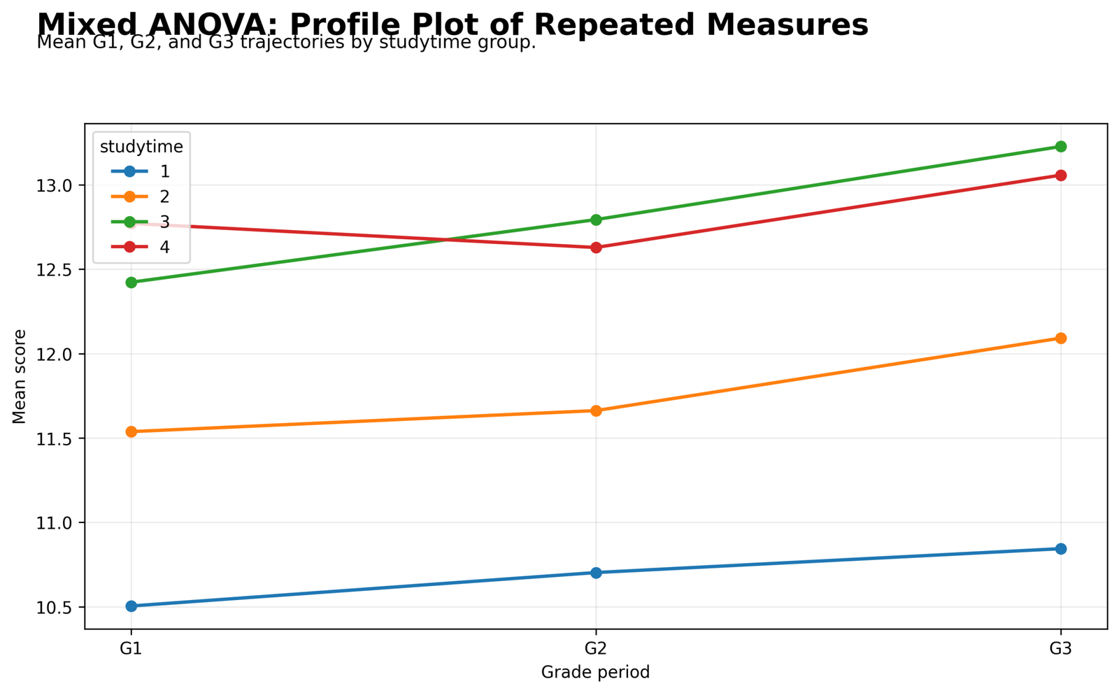
This profile plot shows the repeated grade trajectory for each studytime group. Studytime group 1 stays lowest across G1, G2 and G3, moving from about 10.50 to 10.84. Group 2 is higher, moving from about 11.54 to 12.09. Group 3 is high throughout and ends highest at G3, while group 4 begins high, dips slightly at G2 and rises again at G3.
The vertical separation between the lines explains the significant between-subjects studytime effect. Students in higher studytime groups have higher overall grade profiles than students in group 1.
The lines are not perfectly parallel, but the interaction F statistic is small and non-significant. The chart should therefore be interpreted as strong evidence of group-level differences and overall grade-period change, not as strong evidence that each studytime group changes differently over time.
Python Chart 2: Overall Within-Subject Means
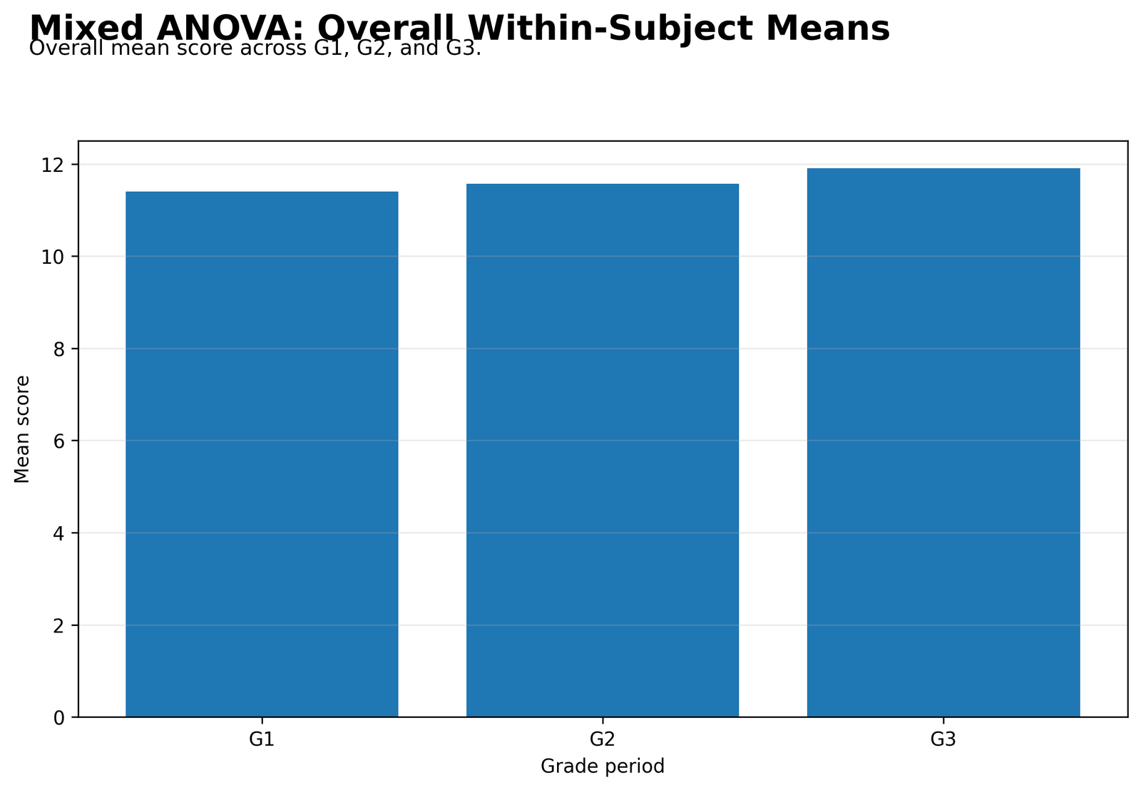
This chart summarizes the repeated-measures pattern after averaging across studytime groups. The overall mean is about 11.40 for G1, about 11.57 for G2 and about 11.91 for G3.
The bar heights rise across the grade periods. This explains the significant within-subject Grade_Period result: scores are not constant across G1, G2 and G3.
This chart is the cleanest visual explanation of the repeated-measures main effect. It shows the overall grade-period increase without the extra group lines from the profile plot.
Python Chart 3: Cell Means Heatmap
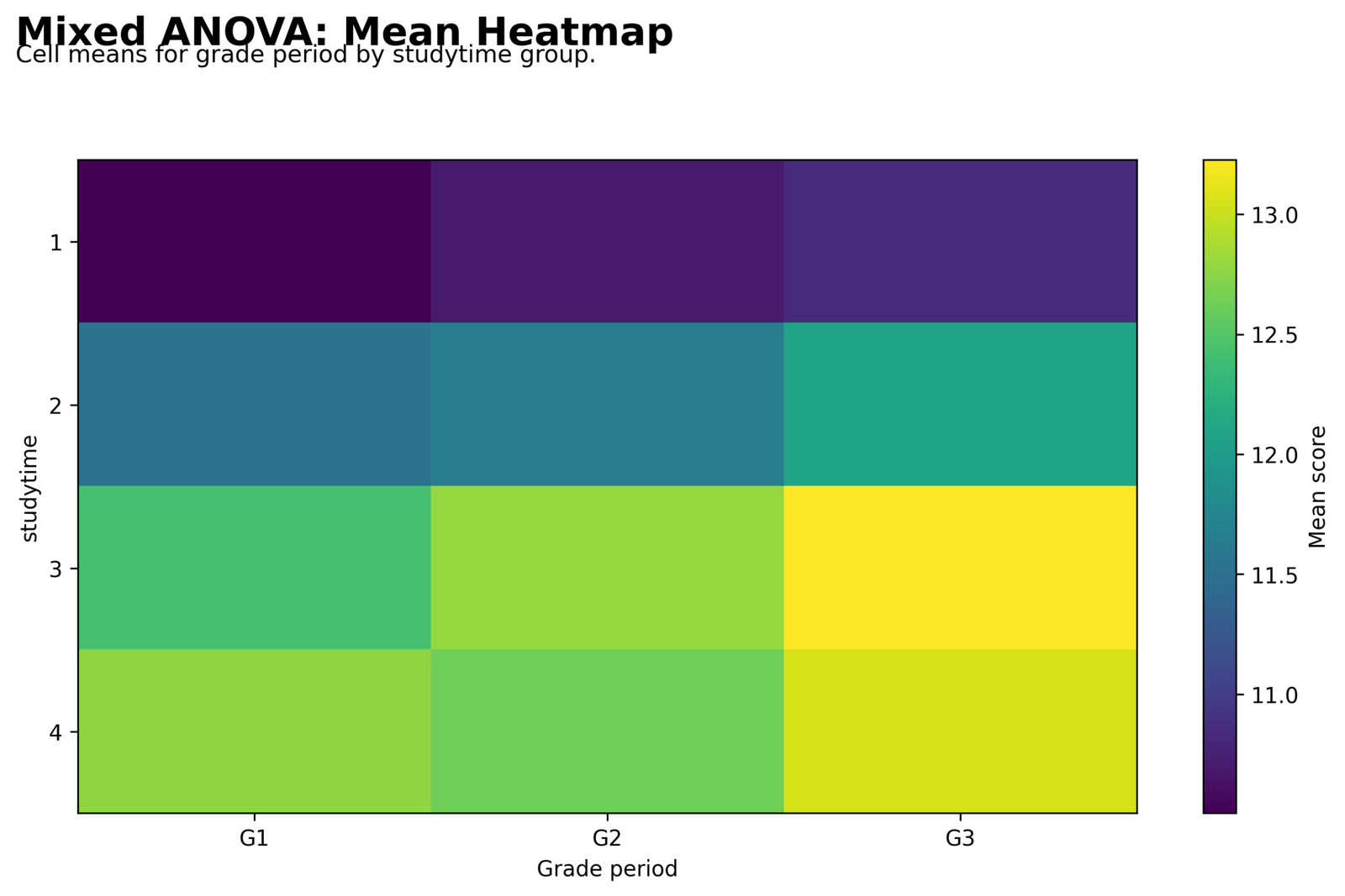
The heatmap gives the group-by-period means in a compact visual form. Studytime group 1 has the lowest values across the row. Group 2 is higher than group 1. Groups 3 and 4 have the highest color intensity, especially at G3.
The exact pattern matches the SPSS descriptive table: group 1 has means of 10.5047, 10.7028 and 10.8443; group 2 has 11.5377, 11.6623 and 12.0918; group 3 has 12.4227, 12.7938 and 13.2268; and group 4 has 12.7714, 12.6286 and 13.0571.
This chart explains the result in practical terms. The significant studytime effect comes from consistent group separation, and the significant Grade_Period effect comes from the upward movement across the repeated measures.
Python Chart 4: Mixed ANOVA F Statistics
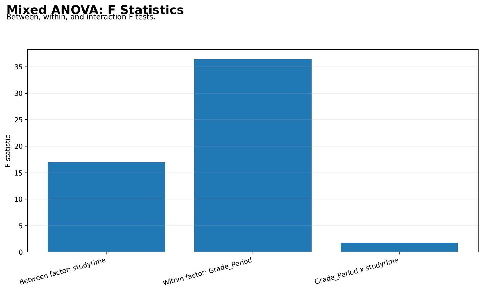
This chart compares the three main Mixed ANOVA F tests. The within-subject Grade_Period effect has the largest F statistic, about 36.41 in the Python chart. The between-subject studytime effect is also large, around 16.98. The interaction is much smaller, around 1.73.
The chart shows the strength ranking of the model effects. Grade_Period and studytime are the main signals. The interaction bar is much shorter, matching the non-significant interaction result in the SPSS table.
This chart is useful for explaining the statistical story quickly: grade scores change across repeated grade periods, studytime groups differ overall, and the group-by-time interaction is weak.
Python Chart 5: Partial Eta Squared for Mixed ANOVA Effects
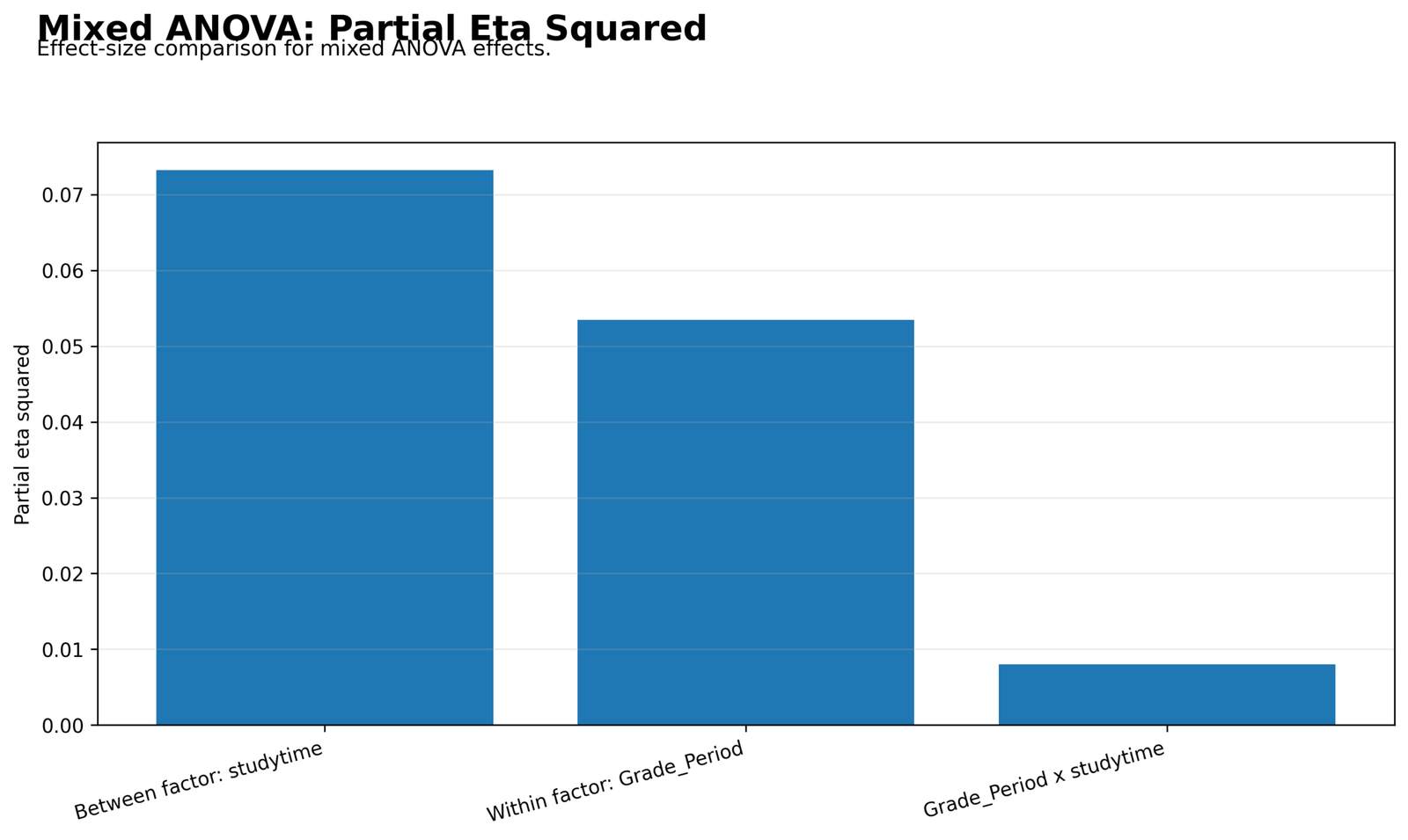
This chart compares the practical effect size of each Mixed ANOVA source. The between-subject studytime effect is largest at about .073. The within-subject Grade_Period effect is smaller but still meaningful. The interaction effect is very small at about .008.
The effect-size chart helps prevent overclaiming. The studytime effect is the strongest practical effect, while the interaction is small.
The correct report should include partial eta squared because an F test alone only gives statistical evidence. Partial eta squared shows how much of the relevant explainable variation is associated with each effect.
Python Chart 6: Within-Subject F Distribution
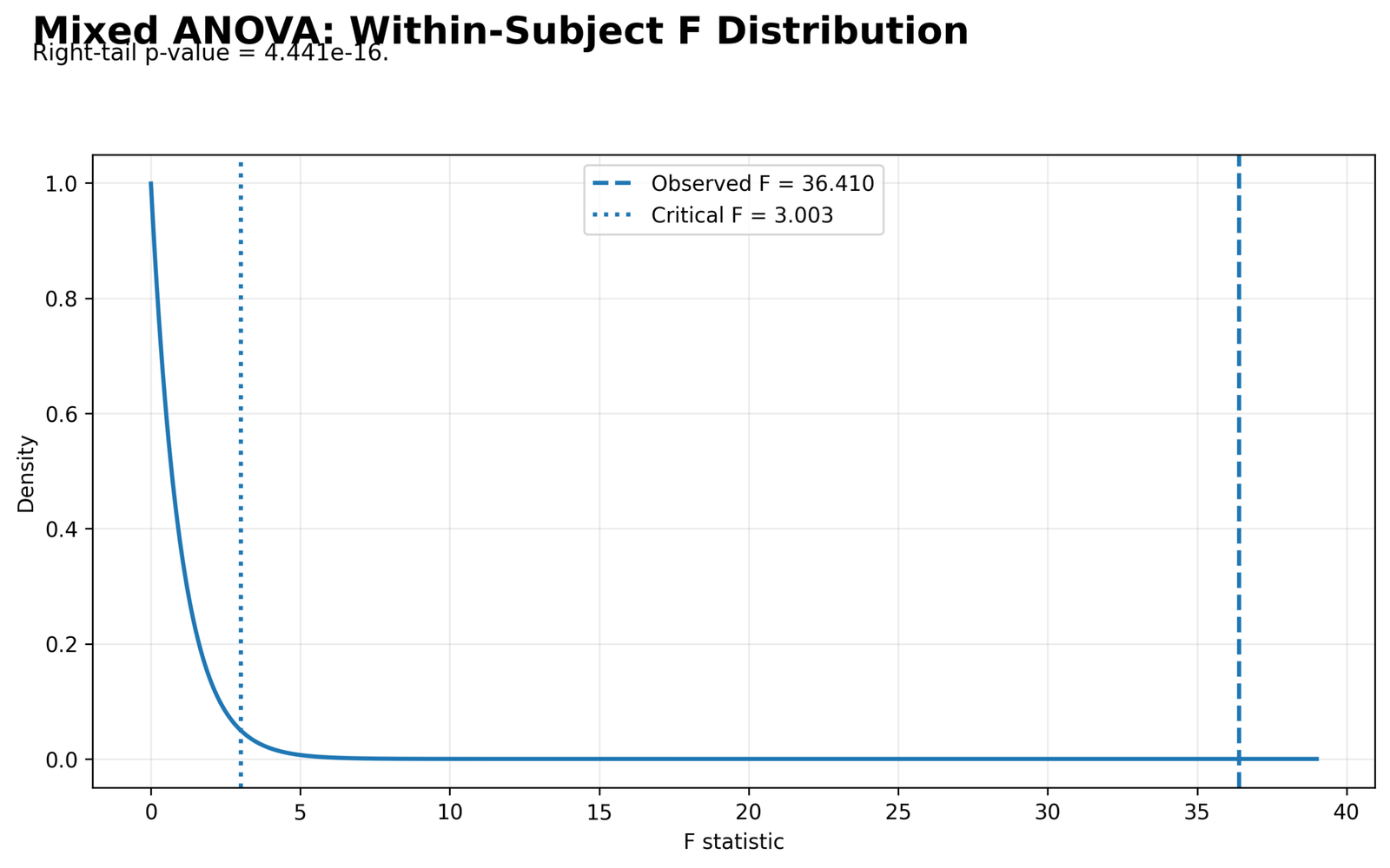
This F distribution chart shows the within-subject Grade_Period decision. The observed F is about 36.410 in the chart, and the critical F is about 3.003. The right-tail p-value is shown as about 4.441e-16.
The observed F line is far to the right of the critical F line. This means the repeated-measures effect is far beyond the rejection threshold.
This chart gives the formal repeated-measures decision visually. The overall scores differ across G1, G2 and G3.
Python Chart 7: Subject Trajectory Spaghetti Plot
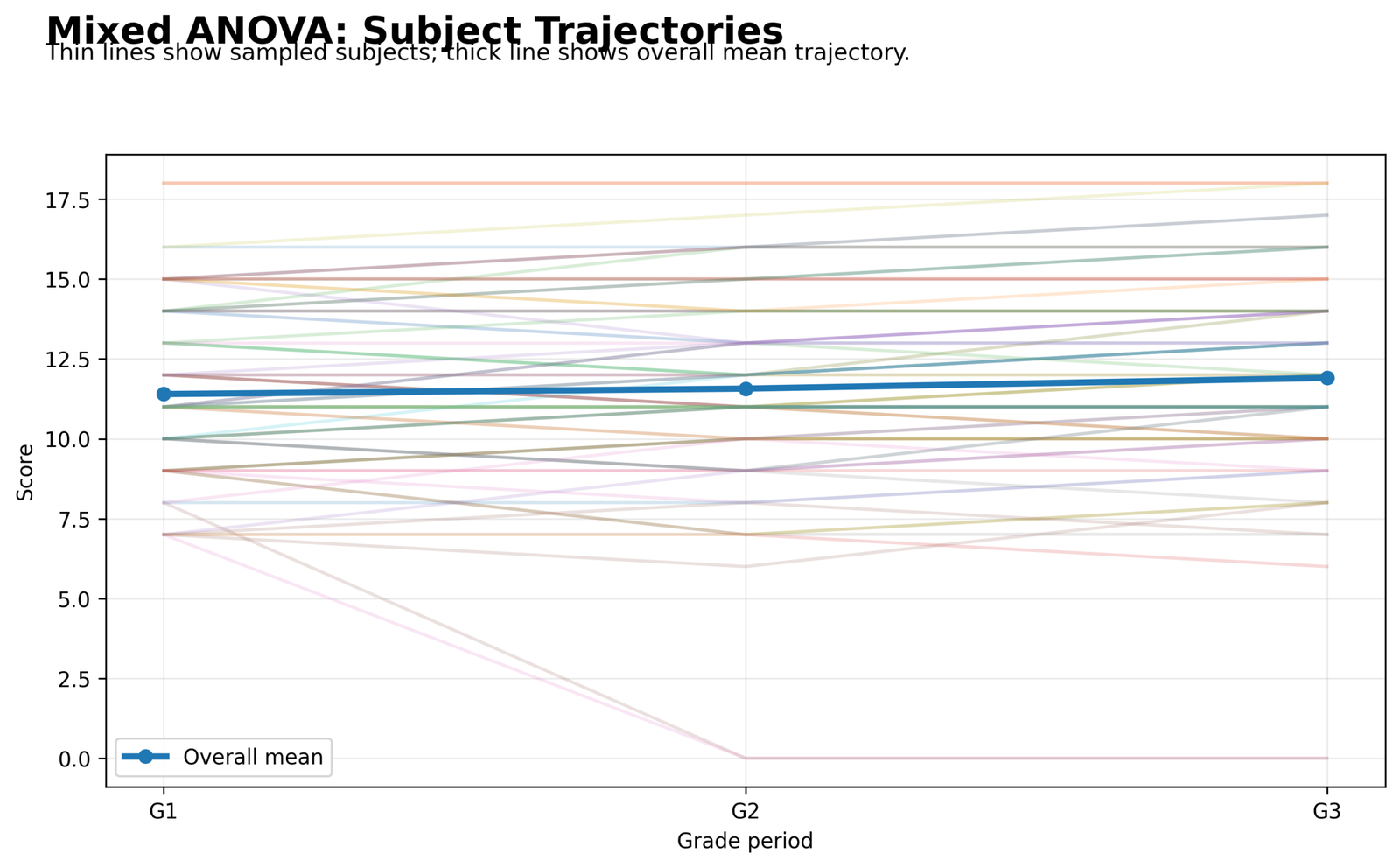
This spaghetti plot shows individual student trajectories across G1, G2 and G3. The thin lines represent sampled students, while the thicker line shows the overall mean trajectory.
The individual lines vary widely. Some students improve, some remain stable, and some decline. A few trajectories fall to very low values, including zero scores. The overall mean line still rises gradually from G1 to G3.
This chart explains why Mixed ANOVA is useful. It handles repeated measurements from the same people while summarizing the overall pattern across many individual trajectories.
Python Chart 8: Difference Score Distributions
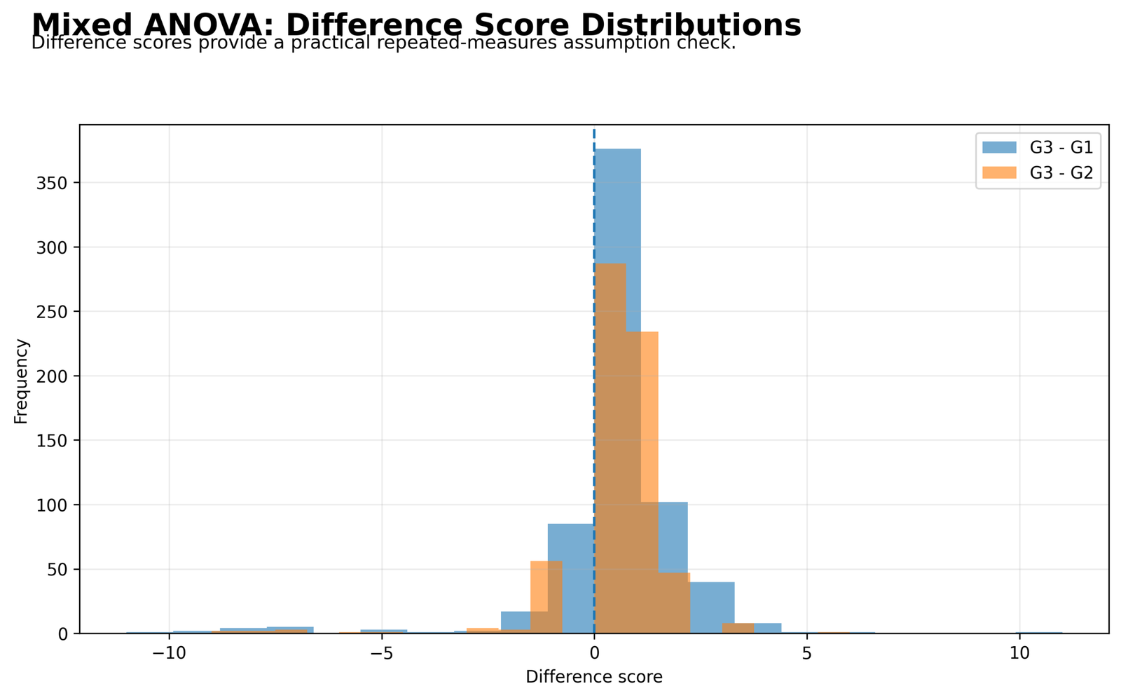
This chart shows the distribution of change scores. The G3 – G1 and G3 – G2 distributions are concentrated near small positive values, which supports the overall increase shown in the within-subject means chart.
The chart also shows extreme negative values, especially for G3 – G1. Those negative differences represent students whose final grade was much lower than an earlier grade. The positive tail shows students who improved strongly.
This chart is a practical repeated-measures check. It shows that the average change is positive, but individual change is not uniform across all students.
R Chart-by-Chart Validation
The R validation charts repeat the same Mixed ANOVA workflow in a second software environment. They confirm the profile plot, within-subject means, cell means, F statistics, partial eta squared, within-subject F distribution, subject trajectories and difference-score pattern.
R Chart 1: Profile Plot of Repeated Measures by Studytime Group
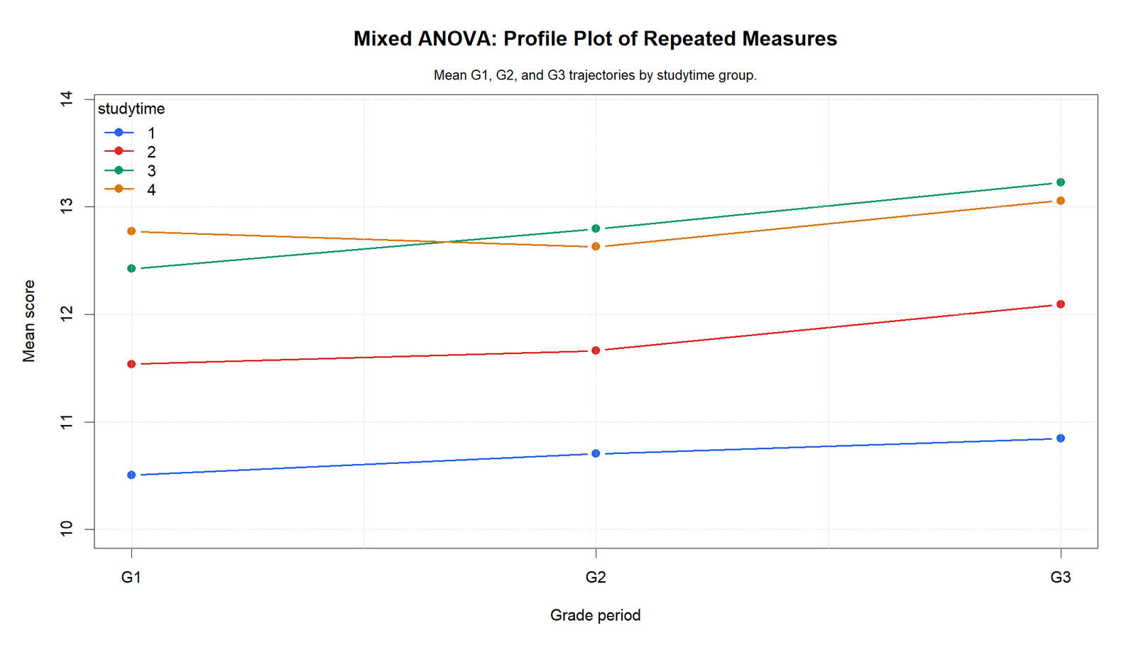
The R profile plot confirms the same pattern as the Python chart. Studytime group 1 remains lowest, group 2 is higher, and groups 3 and 4 are in the higher score range.
The group 4 line dips slightly at G2 and rises again at G3, while group 3 rises more steadily. This creates some non-parallel line movement, but the formal interaction remains small and non-significant.
This validation chart supports the same interpretation: the studytime groups differ overall, and scores change across periods, but the interaction is not the main finding.
R Chart 2: Overall Within-Subject Means
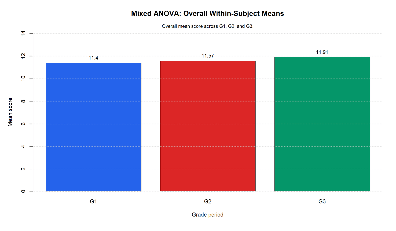
The R bar chart confirms that the overall mean increases from G1 to G3. The values match the SPSS descriptives, with G1 around 11.40, G2 around 11.57 and G3 around 11.91.
This validates the repeated-measures conclusion. The Grade_Period effect is statistically significant because the repeated means do not remain equal.
The chart should be used to explain the within-subject effect in a simple way before discussing sphericity corrections.
R Chart 3: Cell Means Heatmap
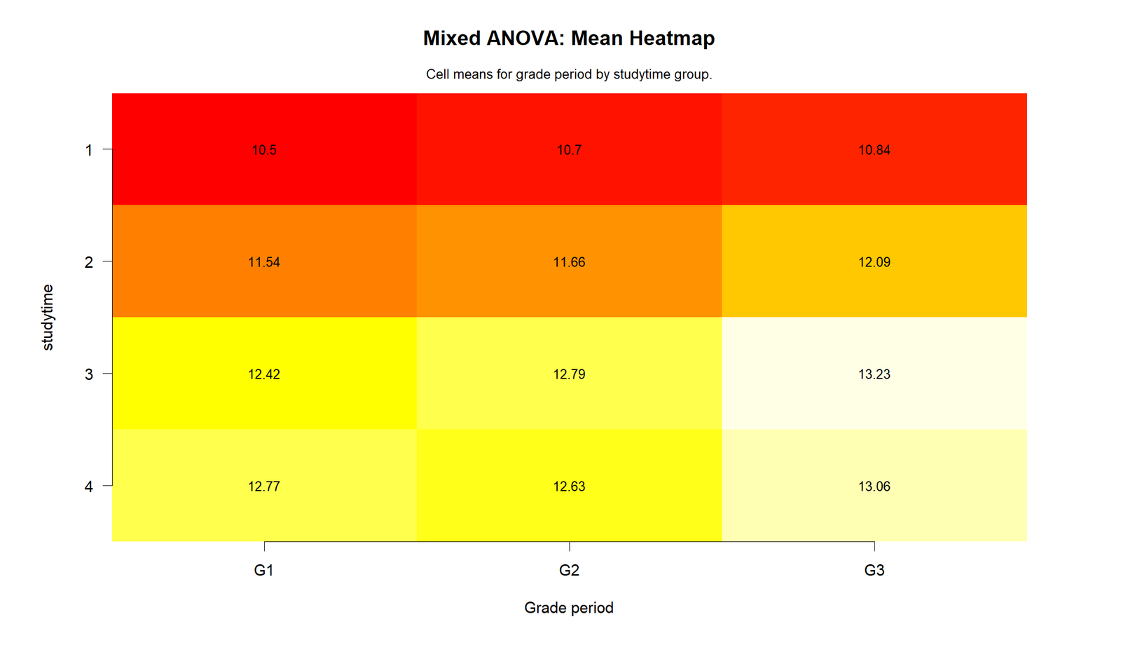
The R heatmap confirms the same cell-mean structure. Studytime group 1 has the lowest row, group 2 is higher, and groups 3 and 4 have the highest values.
The highest G3 mean appears in studytime group 3, while group 4 remains close to that high range. This supports the studytime main effect.
This validation output is useful because it shows the full repeated-measures-by-group mean table in one visual.
R Chart 4: Mixed ANOVA F Statistics
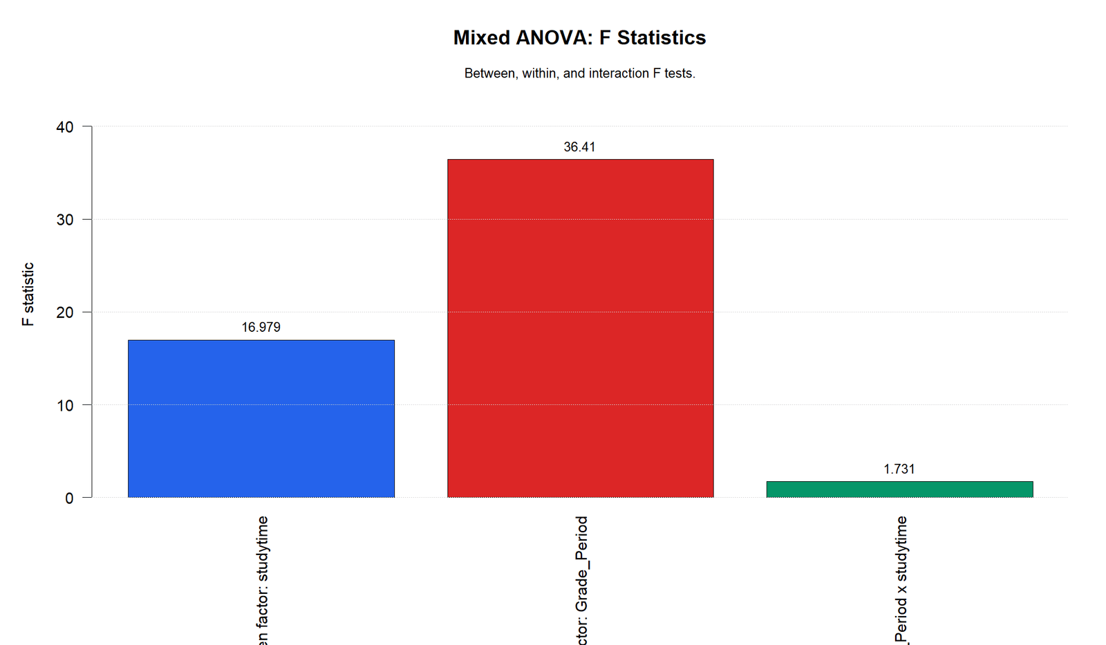
The R F statistic chart labels the main values directly: studytime has F = 16.979, Grade_Period has F = 36.41 in the R chart workflow, and the interaction has F = 1.731.
The same ranking appears again. The repeated-measures effect and studytime effect are clearly larger than the interaction.
This confirms that the interaction should not be over-interpreted. The main results are the between-group studytime difference and the within-student grade-period change.
R Chart 5: Partial Eta Squared
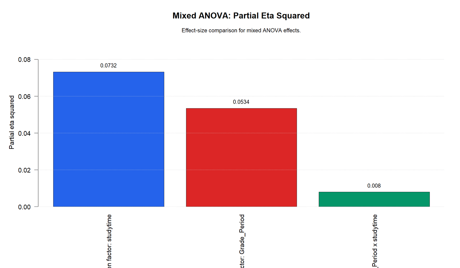
The R effect-size chart confirms that studytime has the largest partial eta squared, Grade_Period has a smaller but meaningful partial eta squared, and the interaction is very small.
This effect-size pattern matches the SPSS output: studytime partial η² is .073, Grade_Period partial η² is .028 in the within-subjects table, and the interaction partial η² is .008.
The final report should state both statistical significance and effect size. This avoids treating every significant test as equally important.
R Chart 6: Within-Subject F Distribution
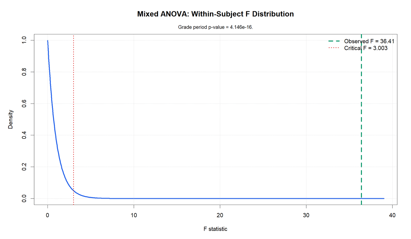
The R F distribution chart shows observed F = 36.41 and critical F = 3.003, with the observed F far to the right of the critical line.
The chart label reports the Grade_Period p-value as about 4.146e-16. This is far below .05 and supports the repeated-measures result.
This chart visually confirms the repeated-measures decision in the R workflow.
R Chart 7: Subject Trajectory Spaghetti Plot
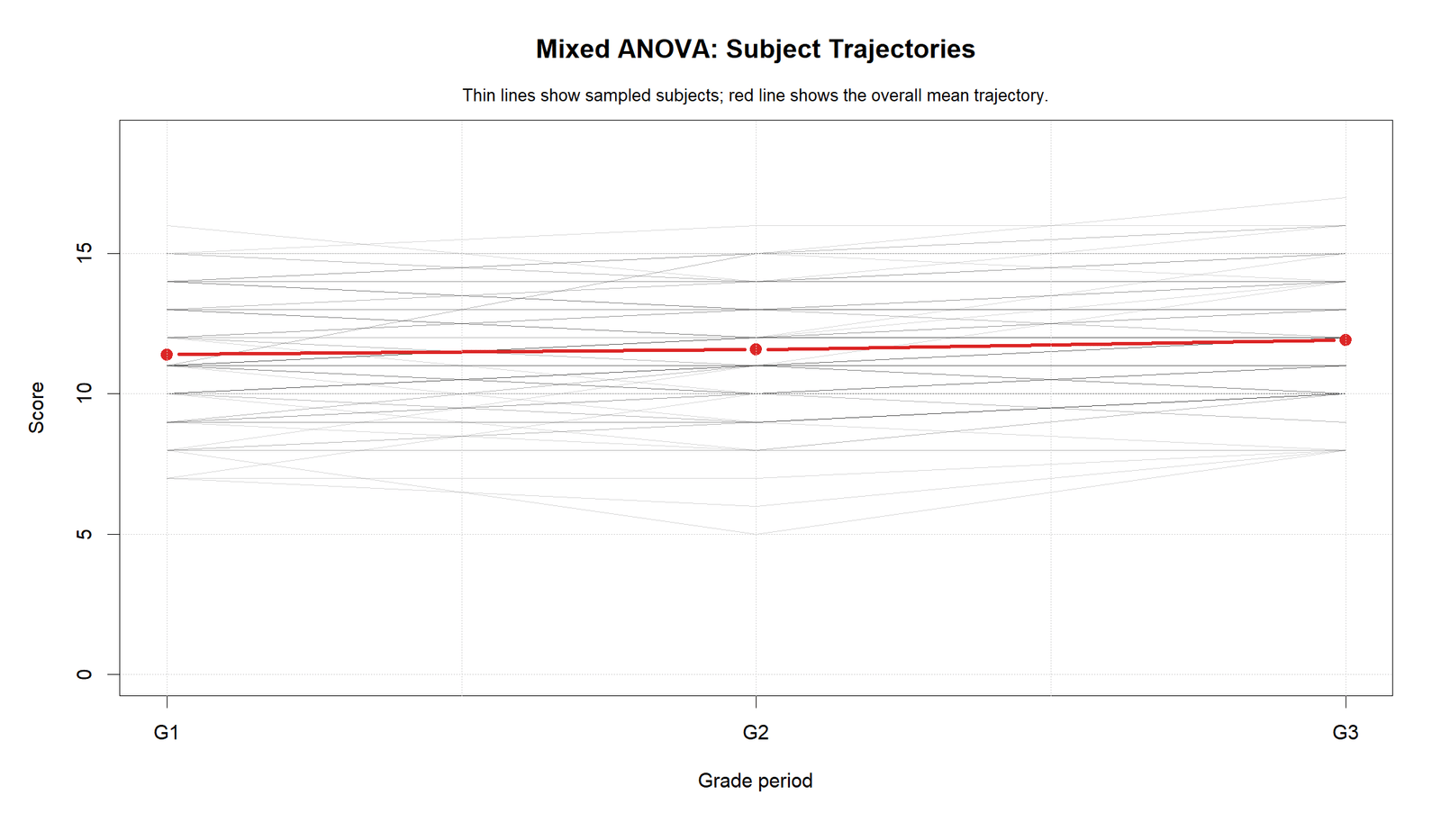
The R trajectory plot confirms that individual student paths vary strongly. Some students improve, others decline, and many remain close to their starting range.
The overall mean trajectory still increases gradually across G1, G2 and G3. This validates the within-subject effect while showing that individual patterns are heterogeneous.
This chart is useful for explaining why repeated-measures models should respect within-person structure rather than treating all grade observations as independent.
R Chart 8: Difference Score Distributions
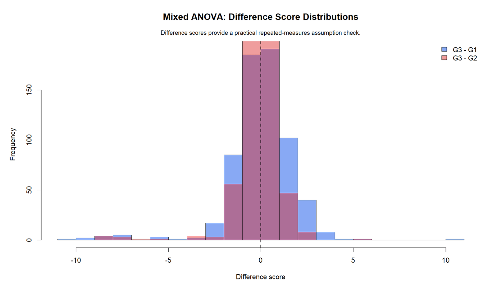
The R difference-score chart confirms that most changes are near small positive values, while a smaller number of students have large negative or positive changes.
The distribution supports the overall Grade_Period effect but also shows that repeated-measures change is not identical for every student.
This chart should be used as a practical diagnostic explanation alongside the formal F test and sphericity discussion.
SPSS Output and Report PDFs
The supplied report files support the Mixed ANOVA workflow. The Python report provides the first chart set, the R report validates the same chart sequence, and the SPSS output PDF provides the repeated-measures GLM tables used for formal reporting.
Download Mixed ANOVA Python Report PDF
Download Mixed ANOVA R Report PDF
Download Mixed ANOVA SPSS Output PDF
SPSS Output Items to Read
| SPSS Output Item | Key Result | How It Is Used | Reporting Meaning |
|---|---|---|---|
| Descriptive statistics | G1 = 11.3991, G2 = 11.5701, G3 = 11.9060 | Describes repeated-measures means. | Scores rise across grade periods. |
| Between-subjects factor table | studytime group sizes 212, 305, 97 and 35 | Shows group balance and sample structure. | Group 4 is smallest. |
| Mauchly’s test | W = .826, p < .001 | Checks sphericity. | Use corrected within-subject rows. |
| Greenhouse-Geisser epsilon | .852 | Corrects degrees of freedom when sphericity is violated. | Corrected result remains significant for Grade_Period. |
| Within-subject Grade_Period | F = 18.865, p < .001, ηp² = .028 | Tests repeated grade change. | Scores change across G1, G2 and G3. |
| Grade_Period × studytime | F = 1.731, p = .110, ηp² = .008 | Tests whether change differs by group. | Interaction is small and non-significant. |
| Between-subjects studytime | F = 16.979, p < .001, ηp² = .073 | Tests overall group differences. | Studytime groups differ overall. |
| Levene tests | G1 p = .653, G2 p = .165, G3 p = .400 | Checks equality of variance by studytime group. | No serious variance violation is shown by mean-based tests. |
SPSS interpretation summary: The repeated-measures GLM output supports a significant studytime effect and a significant Grade_Period effect. Mauchly’s test is significant, so corrected within-subject rows should be reviewed. The Grade_Period effect remains significant after correction, while the interaction remains non-significant.
SPSS, R, Python and Excel Workflows for Mixed ANOVA
The same Mixed ANOVA workflow can be reproduced in SPSS, R and Python. Excel can prepare profile charts, cell means and difference scores, but formal Mixed ANOVA should be run in SPSS, R or Python because the design contains both repeated and between-subjects components.
SPSS Workflow
| Step | SPSS Menu or Syntax | Purpose |
|---|---|---|
| Open data | File > Open > Data | Load G1, G2, G3 and studytime. |
| Run repeated-measures GLM | Analyze > General Linear Model > Repeated Measures | Fit Mixed ANOVA. |
| Name within factor | Grade_Period with 3 levels | Define G1, G2 and G3 as repeated measures. |
| Assign repeated variables | G1, G2, G3 | Map the repeated-measures columns. |
| Add between factor | studytime | Compare independent groups. |
| Request options | Descriptives, effect size, homogeneity tests | Support reporting and assumptions. |
| Read Mauchly | Mauchly’s Test of Sphericity | Decide whether corrections are needed. |
| Read effects | Within-subjects and between-subjects tables | Report Grade_Period, interaction and studytime effects. |
R Workflow
| Step | R Action | Purpose |
|---|---|---|
| Read data | read.csv("dataset.csv") | Load wide-format data. |
| Reshape data | pivot_longer(G1:G3) | Create long-format repeated-measures data. |
| Define subject ID | id column | Track repeated observations from the same student. |
| Define factors | studytime and Grade_Period | Set between and within factors. |
| Run model | afex::aov_ez() or ezANOVA() | Fit Mixed ANOVA with corrections. |
| Report effects | Between, within and interaction rows | State F, p and partial eta squared. |
Python Workflow
| Step | Python Action | Purpose |
|---|---|---|
| Read data | pandas.read_csv() | Load G1, G2, G3 and studytime. |
| Create ID | df["subject_id"] = range(...) | Identify repeated observations. |
| Reshape to long format | melt() | Create Grade_Period and Score columns. |
| Run mixed ANOVA | pingouin.mixed_anova() | Test within, between and interaction effects. |
| Create profile plots | groupby() and charts | Show repeated-measures trajectories by group. |
| Effect size | Partial eta squared | Compare practical strength of effects. |
Excel Workflow
| Excel Task | Formula or Tool | Purpose |
|---|---|---|
| Prepare data | Keep one row per student with G1, G2, G3 and studytime | Use wide repeated-measures format. |
| Mean profile table | PivotTable with studytime rows and G1/G2/G3 means | Create profile plot. |
| Overall within means | =AVERAGE(G1_range), =AVERAGE(G2_range), =AVERAGE(G3_range) | Summarize Grade_Period effect. |
| Difference scores | =G3-G1 and =G3-G2 | Show practical repeated-measures change. |
| Formal Mixed ANOVA | Use SPSS, R or Python | Excel is not recommended for the full test. |
Code Blocks for Mixed ANOVA
SPSS Syntax for Mixed ANOVA
* Mixed ANOVA in SPSS.
* Repeated measures: G1, G2, G3.
* Within-subject factor: Grade_Period.
* Between-subject factor: studytime.

TITLE "Mixed ANOVA: G1 G2 G3 Repeated Measures by Studytime".

GLM G1 G2 G3 BY studytime
  /WSFACTOR=Grade_Period 3 Polynomial
  /METHOD=SSTYPE(3)
  /PLOT=PROFILE(Grade_Period*studytime)
  /PRINT=DESCRIPTIVE ETASQ HOMOGENEITY
  /CRITERIA=ALPHA(.05)
  /WSDESIGN=Grade_Period
  /DESIGN=studytime.

OUTPUT EXPORT
  /CONTENTS EXPORT=VISIBLE
  /PDF DOCUMENTFILE="Mixed-ANOVA-SPSS-Output.pdf".
Python Code for Mixed ANOVA
import pandas as pd
import pingouin as pg

df = pd.read_csv("dataset.csv")

for col in ["G1", "G2", "G3"]:
    df[col] = pd.to_numeric(df[col], errors="coerce")

df["studytime"] = df["studytime"].astype("category")
df = df.dropna(subset=["G1", "G2", "G3", "studytime"]).copy()
df["subject_id"] = range(1, len(df) + 1)

long_df = df.melt(
    id_vars=["subject_id", "studytime"],
    value_vars=["G1", "G2", "G3"],
    var_name="Grade_Period",
    value_name="Score"
)

# Mixed ANOVA
mixed_result = pg.mixed_anova(
    data=long_df,
    dv="Score",
    within="Grade_Period",
    between="studytime",
    subject="subject_id"
)

print(mixed_result)

# Cell means
cell_means = (
    long_df
    .groupby(["studytime", "Grade_Period"])["Score"]
    .mean()
    .reset_index()
)

print(cell_means)

# Difference scores
df["G3_minus_G1"] = df["G3"] - df["G1"]
df["G3_minus_G2"] = df["G3"] - df["G2"]

print(df[["G3_minus_G1", "G3_minus_G2"]].describe())
R Code for Mixed ANOVA
library(tidyverse)
library(afex)

df <- read.csv("dataset.csv")

df$G1 <- as.numeric(df$G1)
df$G2 <- as.numeric(df$G2)
df$G3 <- as.numeric(df$G3)
df$studytime <- as.factor(df$studytime)
df$subject_id <- seq_len(nrow(df))

long_df <- df %>%
  select(subject_id, studytime, G1, G2, G3) %>%
  pivot_longer(
    cols = c(G1, G2, G3),
    names_to = "Grade_Period",
    values_to = "Score"
  ) %>%
  drop_na()

long_df$Grade_Period <- as.factor(long_df$Grade_Period)

# Mixed ANOVA
model <- aov_ez(
  id = "subject_id",
  dv = "Score",
  data = long_df,
  within = "Grade_Period",
  between = "studytime",
  type = 3
)

print(model)

# Cell means
long_df %>%
  group_by(studytime, Grade_Period) %>%
  summarise(
    n = n(),
    mean = mean(Score),
    sd = sd(Score),
    .groups = "drop"
  )
Excel Notes for Mixed ANOVA
Excel can support Mixed ANOVA reporting, but it should not be the main statistical engine.

Useful Excel steps:
1. Keep one row per student.
2. Columns: studytime, G1, G2, G3.
3. Create PivotTable:
   Rows = studytime
   Values = mean G1, mean G2, mean G3
4. Create profile plot from the PivotTable.
5. Calculate overall repeated-measures means:
   =AVERAGE(G1_range)
   =AVERAGE(G2_range)
   =AVERAGE(G3_range)
6. Calculate difference scores:
   =G3-G1
   =G3-G2
7. Run the formal Mixed ANOVA in SPSS, R or Python.
8. Report F, p value, partial eta squared and sphericity correction when needed.
APA Reporting Wording
When reporting Mixed ANOVA, state the within-subject factor, the between-subjects factor, the interaction result, sphericity decision and effect sizes. Report the interaction before overinterpreting separate main effects.
APA-style report: A mixed ANOVA was used to examine grade scores across three repeated grade periods, G1, G2 and G3, with studytime as the between-subjects factor. Mauchly’s test indicated that the sphericity assumption was violated, W = .826, p < .001, so corrected within-subject results were considered. The main effect of Grade_Period was significant, F = 18.865, p < .001, partial η² = .028, showing that scores changed across G1, G2 and G3. The between-subjects effect of studytime was also significant, F = 16.979, p < .001, partial η² = .073. The Grade_Period × studytime interaction was not significant, F = 1.731, p = .110, partial η² = .008.
Short reporting version: Scores changed significantly across G1, G2 and G3, and studytime groups differed overall. The interaction between grade period and studytime was small and not statistically significant, so the main results are the overall repeated-measures change and the overall studytime group difference.
Common Mistakes
| Mistake | Why It Is Wrong | Correct Practice |
|---|---|---|
| Treating G1, G2 and G3 as independent columns | They are repeated measurements from the same students. | Use repeated-measures structure with a subject ID. |
| Ignoring the interaction | The interaction tests whether change differs across groups. | Report Grade_Period × studytime before overexplaining main effects. |
| Ignoring sphericity | Mauchly’s test is significant in this output. | Check Mauchly’s Test of Sphericity, Greenhouse-Geisser Correction and Huynh-Feldt Correction. |
| Reporting only p values | P values do not show practical magnitude. | Report Eta Squared, partial eta squared or Cohen’s F Formula. |
| Claiming strong interaction from non-parallel lines alone | The formal interaction p value is .110. | State that line differences are visible, but interaction is not significant at .05. |
| Using Excel as the final test engine | Excel does not provide a full standard Mixed ANOVA workflow. | Use SPSS, R or Python for the formal model. |
When to Use Mixed ANOVA
Use Mixed ANOVA when the same participants are measured more than once and those participants also belong to different independent groups. In this example, G1, G2 and G3 are repeated measurements, while studytime is a between-subjects grouping factor.
| Situation | Use Mixed ANOVA? | Reporting Note |
|---|---|---|
| Same participants measured at multiple time points | Yes | Define a within-subject factor. |
| Participants also belong to groups | Yes | Define a between-subject factor. |
| Only one repeated group and no between factor | Use repeated-measures ANOVA | Mixed ANOVA is not necessary. |
| Only independent groups and one outcome | Use one-way ANOVA | See ANOVA in Python. |
| Need to include a covariate | Use repeated-measures ANCOVA or mixed model | See ANCOVA. |
Mixed ANOVA is part of the broader ANOVA family. Compare it with Fixed Effects ANOVA, Factorial ANOVA, Balanced ANOVA, Brown Forsythe ANOVA, ANOVA in SPSS, ANOVA in R, ANOVA Effect Size, and ANOVA Assumptions.
Downloads and Resources for Mixed ANOVA
Use these resources to reproduce the Mixed ANOVA workflow. The Python report, R report and SPSS output PDF are included as verification files. Script and workbook placeholders can be replaced after the final downloadable files are uploaded to the WordPress Media Library.
Download Dataset
Practice dataset with studytime, G1, G2 and G3 variables.
Download Mixed ANOVA Python Report PDF
Python report PDF for profile plots, F statistics, effect sizes and diagnostics.
Download Mixed ANOVA R Report PDF
R validation PDF for Mixed ANOVA charts and repeated-measures interpretation.
Download Mixed ANOVA SPSS Output PDF
SPSS output PDF for repeated-measures GLM, sphericity and effect sizes.
Download Python Script
Python code for Mixed ANOVA, profile plots, partial eta squared and difference scores.
Download R Script and Excel Workbook
R workflow and Excel support workbook for Mixed ANOVA summaries.
FAQs About Mixed ANOVA
What is Mixed ANOVA?
Mixed ANOVA is an ANOVA design that includes one repeated-measures factor and one between-subjects factor. It tests within-subject change, group differences and the interaction between change and group.
What variables were used in this Mixed ANOVA example?
The repeated-measures variables were G1, G2 and G3. The within-subject factor was Grade_Period, and the between-subjects factor was studytime.
Was the studytime effect significant?
Yes. The between-subjects studytime effect was significant, F = 16.979, p < .001, partial η² = .073.
Was the Grade_Period effect significant?
Yes. The within-subject Grade_Period effect was significant, F = 18.865, p < .001, partial η² = .028.
Was the Grade_Period by studytime interaction significant?
No. The interaction was small and not statistically significant under the sphericity-assumed row, F = 1.731, p = .110, partial η² = .008.
What did Mauchly’s test show?
Mauchly’s test was significant, W = .826, p < .001. This means sphericity was violated, so Greenhouse-Geisser and Huynh-Feldt corrections should be checked.
What did the profile plot show?
The profile plot showed that studytime group 1 had the lowest grade profile, group 2 was higher, and groups 3 and 4 were in the highest range. Most groups increased from G1 to G3.
Can Mixed ANOVA be done in Excel?
Excel can create profile plots, cell means and difference-score summaries, but the formal Mixed ANOVA should be run in SPSS, R or Python.
Can Mixed ANOVA be done in SPSS?
Yes. Use Analyze > General Linear Model > Repeated Measures, define Grade_Period with three levels, assign G1, G2 and G3, and add studytime as the between-subjects factor.
How do I report this Mixed ANOVA in APA style?
A concise report is: A Mixed ANOVA showed significant effects of Grade_Period and studytime on grade scores, while the Grade_Period × studytime interaction was not significant.

