
SPSS One-Way ANOVA, Descriptives, Levene Test, Tukey HSD, Effect Size and Residual Diagnostics
ANOVA in SPSS: One-Way ANOVA, Formula, Output, Post Hoc, Assumptions and Interpretation
ANOVA in SPSS is used to compare the mean of a numeric outcome across three or more groups. This guide explains how to run a one-way ANOVA in SPSS, how to read the SPSS descriptives table, how to interpret Levene’s homogeneity test, how to report the ANOVA table, how to explain Tukey HSD post hoc results, how to use GLM output for partial eta squared, how to inspect residual diagnostics and how to write the result in APA format. The worked example compares G3 final grade across four studytime groups.
Quick Answer: ANOVA in SPSS Result
The worked ANOVA in SPSS output compares G3 final grade across four studytime groups. The valid sample contains 649 cases, with no excluded cases in the main means output. The group means are 10.84 for studytime group 1, 12.09 for group 2, 13.23 for group 3 and 13.06 for group 4.
The SPSS ANOVA table reports F(3, 645) = 15.876 with Sig. = .000, which should be reported as p < .001. This means the studytime groups do not all have the same mean G3 score. The GLM output reports partial eta squared = .069, so studytime explains about 6.9% of the G3 variation in this one-way model.
Final interpretation: The SPSS one-way ANOVA shows a statistically significant difference in G3 final grade across studytime groups. The highest mean appears in studytime group 3, while the lowest mean appears in studytime group 1. The post hoc output shows that group 1 differs significantly from groups 2, 3 and 4, while groups 3 and 4 are not significantly different from each other.
Important reporting point: SPSS displays p values as .000 in several tables. In a statistical report, this should be written as p < .001, not p = .000. A complete SPSS ANOVA report should include group means, Levene’s test, F statistic, degrees of freedom, p value, effect size and post hoc interpretation.
Table of Contents
- What Is ANOVA in SPSS?
- ANOVA Formula Used in SPSS
- Null and Alternative Hypothesis
- Dataset and SPSS Variables Used
- SPSS Output-by-Output Interpretation
- SPSS Workflow for One-Way ANOVA
- SPSS, R, Python and Excel Workflows
- Code Blocks for ANOVA in SPSS
- APA Reporting Wording
- Common Mistakes
- When to Use ANOVA in SPSS
- Downloads and Resources
- Related Guides
- FAQs
What Is ANOVA in SPSS?
ANOVA in SPSS is a mean-comparison procedure used when one numeric dependent variable is compared across three or more categories of a grouping variable. In this guide, the dependent variable is G3 final grade, and the grouping variable is studytime with four categories.
SPSS can run this analysis through Analyze > Compare Means > One-Way ANOVA or through Analyze > General Linear Model > Univariate. The One-Way ANOVA menu is useful for descriptives, Levene’s test and Tukey HSD post hoc comparisons. The GLM menu is useful because it reports effect size through partial eta squared.
The SPSS output in this article includes descriptives, homogeneity tests, the ANOVA table, Tukey post hoc comparisons, homogeneous subsets, estimated marginal means, GLM effect size, residual diagnostics, boxplots, a means plot and residual charts. These sections together explain the statistical result, group direction, practical size and diagnostic quality of the model.
Simple definition: ANOVA in SPSS tests whether three or more group means are equal. In this example, SPSS tests whether mean G3 final grade differs across four studytime groups.
Before reading SPSS ANOVA output, it helps to understand Descriptive Statistics, Mean Median and Mode, Standard Deviation, Variance, Standard Error, Confidence Interval, P Value, and Null and Alternative Hypothesis.
ANOVA Formula Used in SPSS
A one-way ANOVA model can be written as:
In this formula, Yij is the observed G3 score for student j in studytime group i, μ is the grand mean, τi is the studytime group effect, and εij is the residual error.
SPSS ANOVA F Statistic
The SPSS ANOVA table reports SS between = 465.078, df between = 3, MS between = 155.026, SS within = 6298.189, df within = 645 and MS within = 9.765. Dividing 155.026 by 9.765 gives the reported F statistic of 15.876.
Partial Eta Squared Formula
The GLM output reports partial eta squared = .069 for studytime. This means studytime accounts for about 6.9% of the effect-plus-error variation in G3 in this one-way model.
| SPSS Term | Value in This Output | Meaning | Reporting Use |
|---|---|---|---|
| Dependent variable | G3 | Final grade being compared. | State as the outcome variable. |
| Factor | studytime | Four studytime groups. | State as the grouping factor. |
| Between-groups SS | 465.078 | Variation explained by studytime. | Used in ANOVA and effect-size formulas. |
| Within-groups SS | 6298.189 | Variation left inside groups. | Used as the error variation. |
| F statistic | 15.876 | Between-group mean square divided by within-group mean square. | Report with df and p value. |
| Partial eta squared | .069 | Effect-size measure from GLM output. | Report as a medium-sized practical effect. |
Null and Alternative Hypothesis for ANOVA in SPSS
The SPSS one-way ANOVA tests whether mean G3 is equal across all four studytime groups. The null hypothesis says that the group means are equal. The alternative hypothesis says that at least one group mean is different.
| Hypothesis | Statement | Meaning for This SPSS Output |
|---|---|---|
| Null hypothesis | H0: μ1 = μ2 = μ3 = μ4 | All studytime groups have the same mean G3 score. |
| Alternative hypothesis | H1: at least one mean differs | At least one studytime group has a different mean G3 score. |
| SPSS decision evidence | F(3,645) = 15.876, p < .001 | Reject the null hypothesis. |
| Practical evidence | Partial η² = .069 | The studytime effect has a meaningful medium-sized interpretation. |
Decision for this example: The SPSS ANOVA result rejects the null hypothesis. Mean G3 is not equal across all studytime groups. Tukey and pairwise comparison output show that group 1 is significantly lower than groups 2, 3 and 4, and group 2 is significantly lower than group 3.
Dataset and SPSS Variables Used
The worked example uses a student performance dataset. The dependent variable is G3 final grade, and the factor is studytime. The case processing summaries show 649 valid cases and no missing or excluded cases in the shown SPSS means and residual outputs.
| Variable or Output | Role | Why It Matters in SPSS ANOVA | Where It Appears |
|---|---|---|---|
| G3 | Dependent variable | Numeric final-grade score being compared. | Descriptives, ANOVA table, residuals and charts. |
| studytime | Grouping factor | Defines four groups in the one-way ANOVA. | Means table, Tukey output, GLM and plots. |
| Levene statistic | Homogeneity test | Checks whether error variances are similar. | Test of Homogeneity of Variances. |
| Tukey HSD | Post hoc test | Shows which studytime groups differ after significant ANOVA. | Multiple Comparisons table. |
| Partial eta squared | Effect size | Shows practical magnitude of the studytime effect. | GLM Tests of Between-Subjects Effects table. |
| Residuals | Model errors | Used for normality and model-diagnostic checks. | Explore output, Q-Q plots, residual plots and histogram. |
For supporting concepts, review ANOVA Assumptions, ANOVA Effect Size, ANOVA in Python, ANOVA in R, Levene Test, Effect Size, Box Plot Interpretation, and Q-Q Plot Normality Check.
SPSS Output-by-Output Interpretation
The SPSS output pages below show the complete one-way ANOVA workflow. The sequence begins with descriptive group statistics, then moves to homogeneity testing, the ANOVA table, Tukey HSD post hoc comparisons, GLM effect size, estimated marginal means, residual diagnostics, group boxplots, means plot and residual charts.
SPSS Output PDF: Complete ANOVA File
Download ANOVA in SPSS Output PDF
The PDF is the complete verification file for the SPSS workflow. It contains the one-way ANOVA output, GLM output, post hoc tables, homogeneous subsets, residual diagnostics and charts used in this article. Readers can use the PDF to confirm the reported values instead of relying only on the article summary.
SPSS Page 5: Means Report and Case Processing Summary
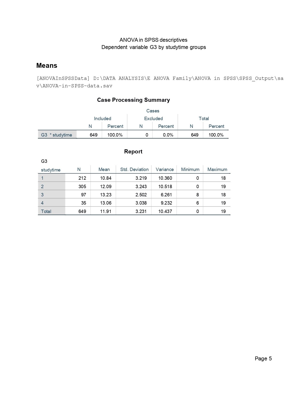
This SPSS page shows that all 649 cases were included and no cases were excluded. The report table gives the first direct comparison of G3 across studytime groups. Group 1 has a mean of 10.84, group 2 has a mean of 12.09, group 3 has a mean of 13.23, and group 4 has a mean of 13.06.
The values show that G3 increases from studytime group 1 to group 3, with group 4 staying close to group 3. The standard deviations are 3.219, 3.243, 2.502 and 3.038, so the spread is broadly similar across groups, although group 3 has the smallest standard deviation.
This page should be used as the descriptive starting point of the SPSS article. It tells the reader where the group difference is located before the ANOVA table tests whether that difference is statistically significant.
SPSS Page 7: Descriptives and Test of Homogeneity of Variances
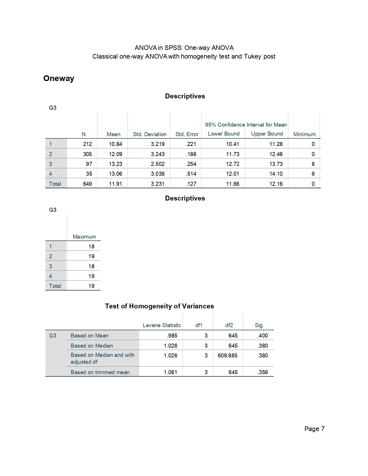
This page gives the one-way ANOVA descriptives with 95% confidence intervals. Group 1 has a 95% confidence interval from 10.41 to 11.28, group 2 from 11.73 to 12.46, group 3 from 12.72 to 13.73, and group 4 from 12.01 to 14.10.
The lower and upper bounds confirm that group 1 is clearly lower than the higher studytime groups. Group 4 has the widest confidence interval because it has only 35 cases, so its mean is less precise than the other groups.
The Levene table supports the equal-variance assumption. The “Based on Mean” row reports Levene statistic = .985 with p = .400, and the median-based row reports p = .380. Since these p values are above .05, the SPSS output supports homogeneity of variance for ordinary one-way ANOVA.
SPSS Page 8: ANOVA Table and Tukey HSD Multiple Comparisons
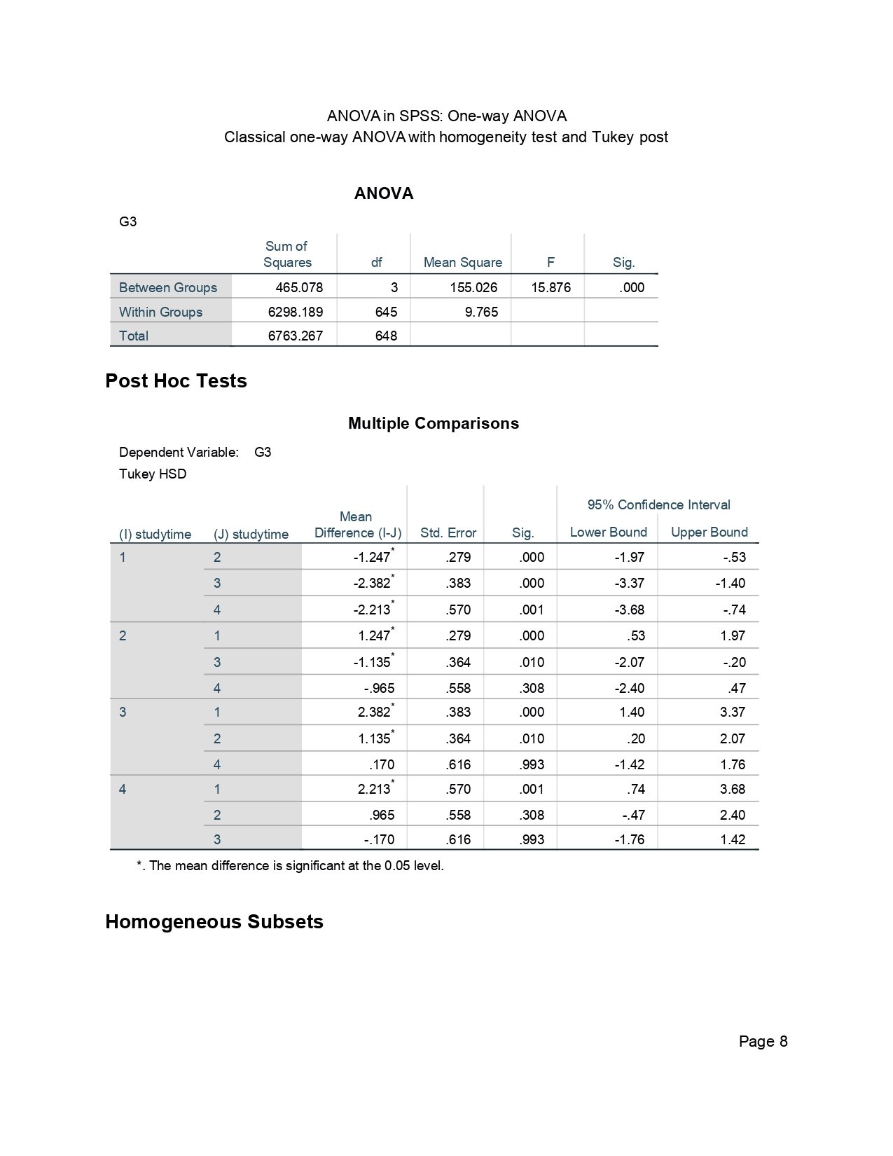
This page contains the main SPSS ANOVA table. Between-groups sum of squares is 465.078, within-groups sum of squares is 6298.189, and the total sum of squares is 6763.267. The ANOVA result is F(3,645) = 15.876 with Sig. = .000, which should be written as p < .001.
The Tukey HSD table explains which pairs differ. Studytime group 1 is significantly lower than group 2 by 1.247 points, lower than group 3 by 2.382 points and lower than group 4 by 2.213 points. Group 2 is also significantly lower than group 3 by 1.135 points.
The non-significant comparisons are also important. Group 2 versus group 4 has p = .308, and group 3 versus group 4 has p = .993. This means the strongest SPSS post hoc conclusion is that the lowest studytime group differs from all higher groups, while the two highest groups are not meaningfully separated from each other.
SPSS Page 9: Homogeneous Subsets
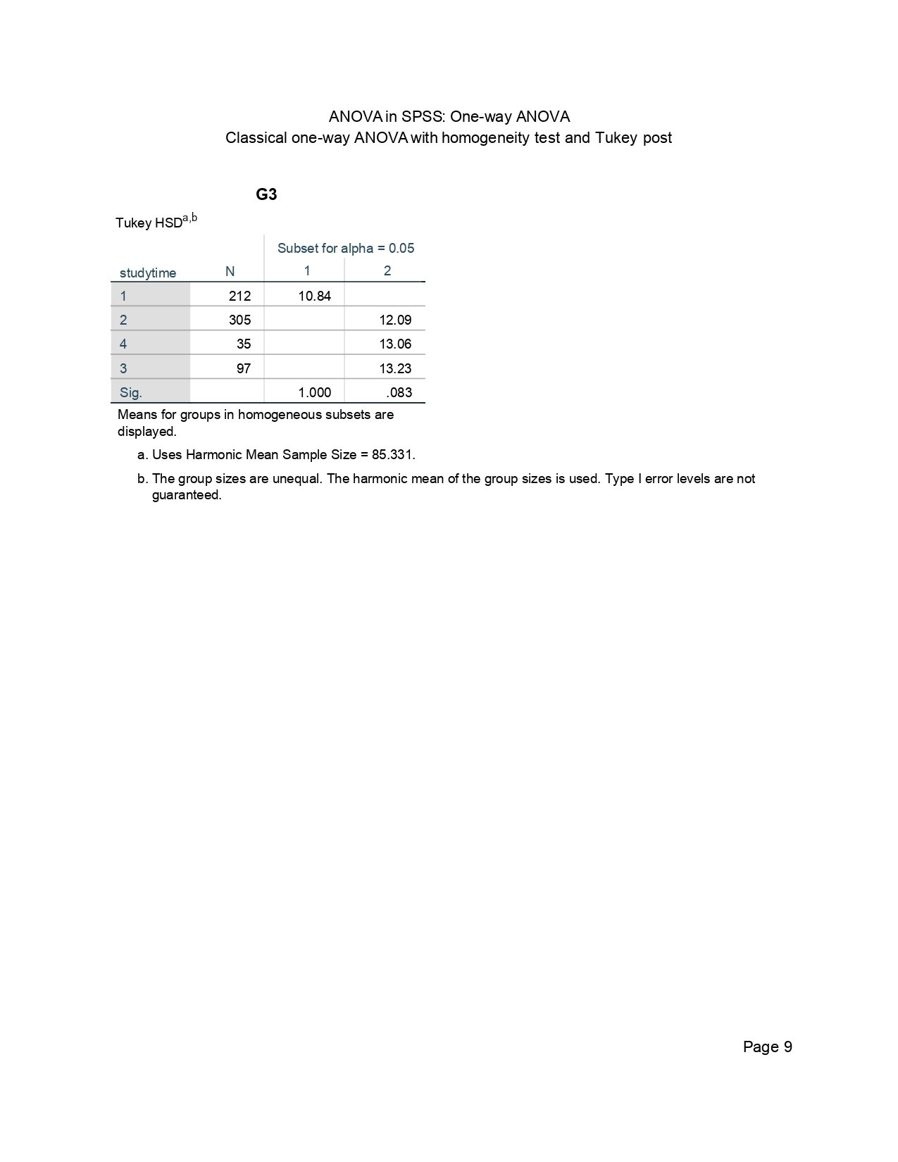
This page groups the studytime categories into homogeneous subsets. Studytime group 1 appears in the first subset with a mean of 10.84. Studytime groups 2, 4 and 3 appear together in the second subset with means of 12.09, 13.06 and 13.23.
The subset result matches the Tukey HSD interpretation. Group 1 is separated from the higher groups, while groups 2, 3 and 4 are close enough to be placed together in a higher subset at alpha = .05. The subset significance for the second subset is .083, which indicates that those groups can be treated as statistically homogeneous within that subset.
This table is useful for a plain-language summary. It shows that the practical split in this output is not four completely separate groups. The main separation is between studytime group 1 and the higher studytime groups.
SPSS Page 11: GLM Descriptives and Levene Test
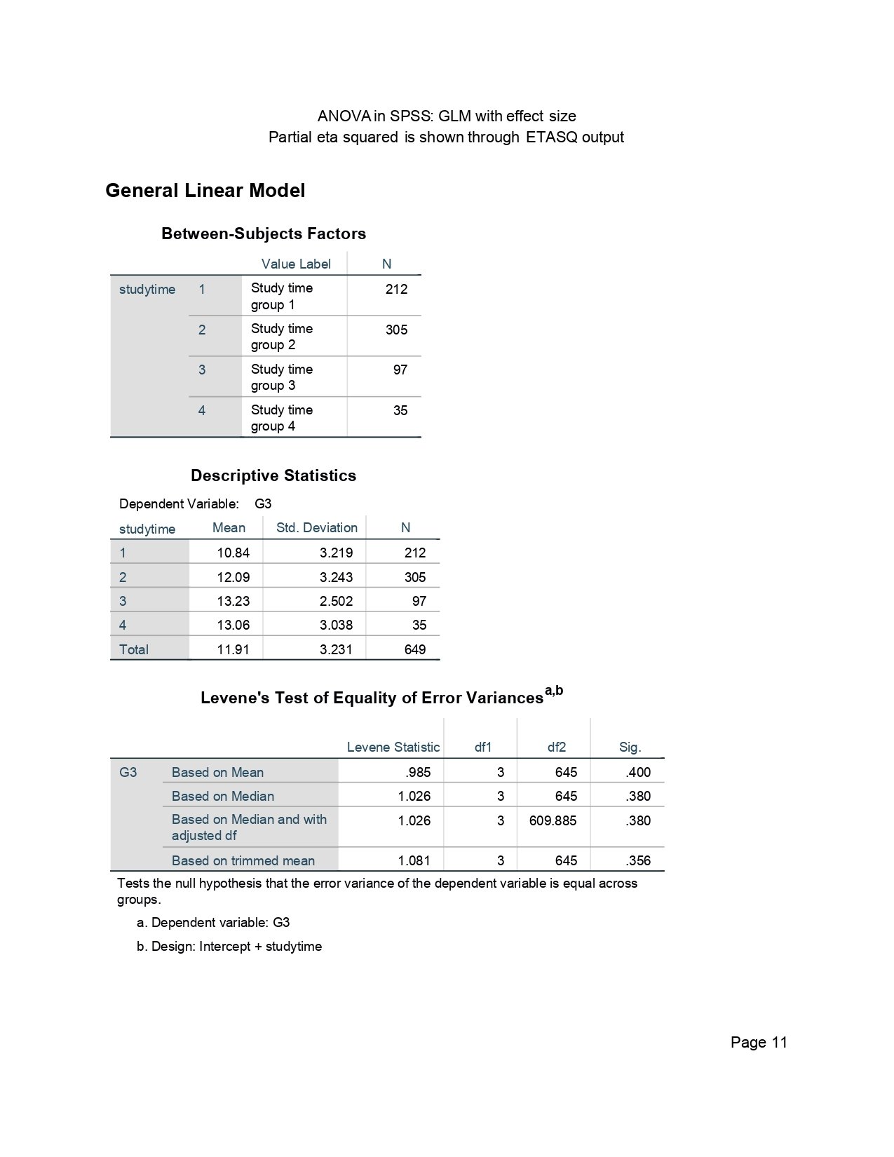
This GLM page repeats the studytime group counts and descriptive statistics. Group 1 has 212 cases, group 2 has 305, group 3 has 97, and group 4 has 35. The same group means appear again: 10.84, 12.09, 13.23 and 13.06.
The Levene table again supports equal variances. The mean-based test gives p = .400, median-based tests give p = .380, and the trimmed mean row gives p = .356. All are above .05.
This page is important because it verifies that the GLM route and the One-Way ANOVA route are using the same studytime groups and the same descriptive pattern. The GLM output is especially useful because it provides partial eta squared on the next pages.
SPSS Page 12: Tests of Between-Subjects Effects and Parameter Estimates
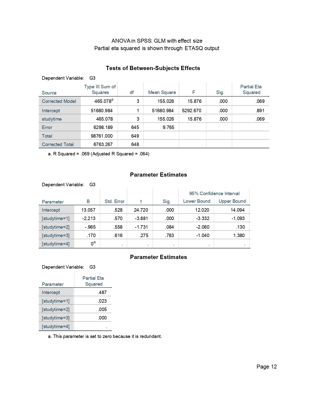
This page gives the GLM version of the ANOVA result. The studytime row reports Type III SS = 465.078, df = 3, F = 15.876, Sig. = .000 and partial eta squared = .069. The corrected model has the same F value and the same effect size because the one-way model has one factor.
The parameter estimates use studytime group 4 as the reference group. Group 1 has B = -2.213, p < .001, showing that group 1 is significantly lower than group 4. Group 2 has B = -.965, p = .084, so group 2 is not significantly different from group 4 in this GLM parameterization. Group 3 has B = .170, p = .783, so group 3 is also not significantly different from group 4.
This page should be used for effect-size reporting. The correct SPSS-style sentence is that the studytime effect was significant, F(3,645) = 15.876, p < .001, partial η² = .069.
SPSS Page 14: Estimated Marginal Means Setup and GLM Result
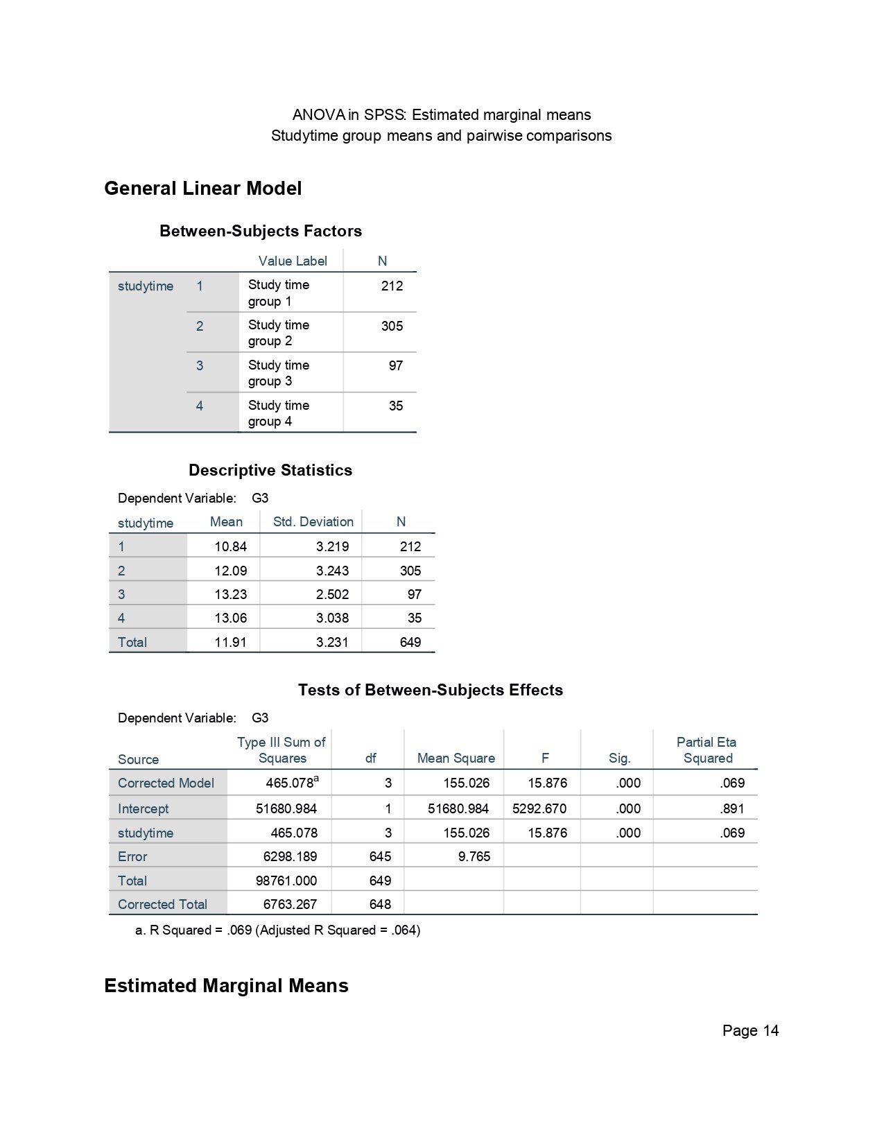
This page repeats the between-subjects factor counts, descriptive means and the tests of between-subjects effects. It again shows that studytime has a significant effect on G3, with F = 15.876, p < .001 and partial eta squared = .069.
The page confirms that the estimated marginal means section is based on the same GLM model. Because this is a one-way design without covariates, the estimated marginal means match the group means shown earlier.
In reporting, this page supports consistency between the ordinary means output and the GLM estimated means output. The result remains the same across SPSS procedures.
SPSS Page 15: Estimated Marginal Means and Pairwise Comparisons
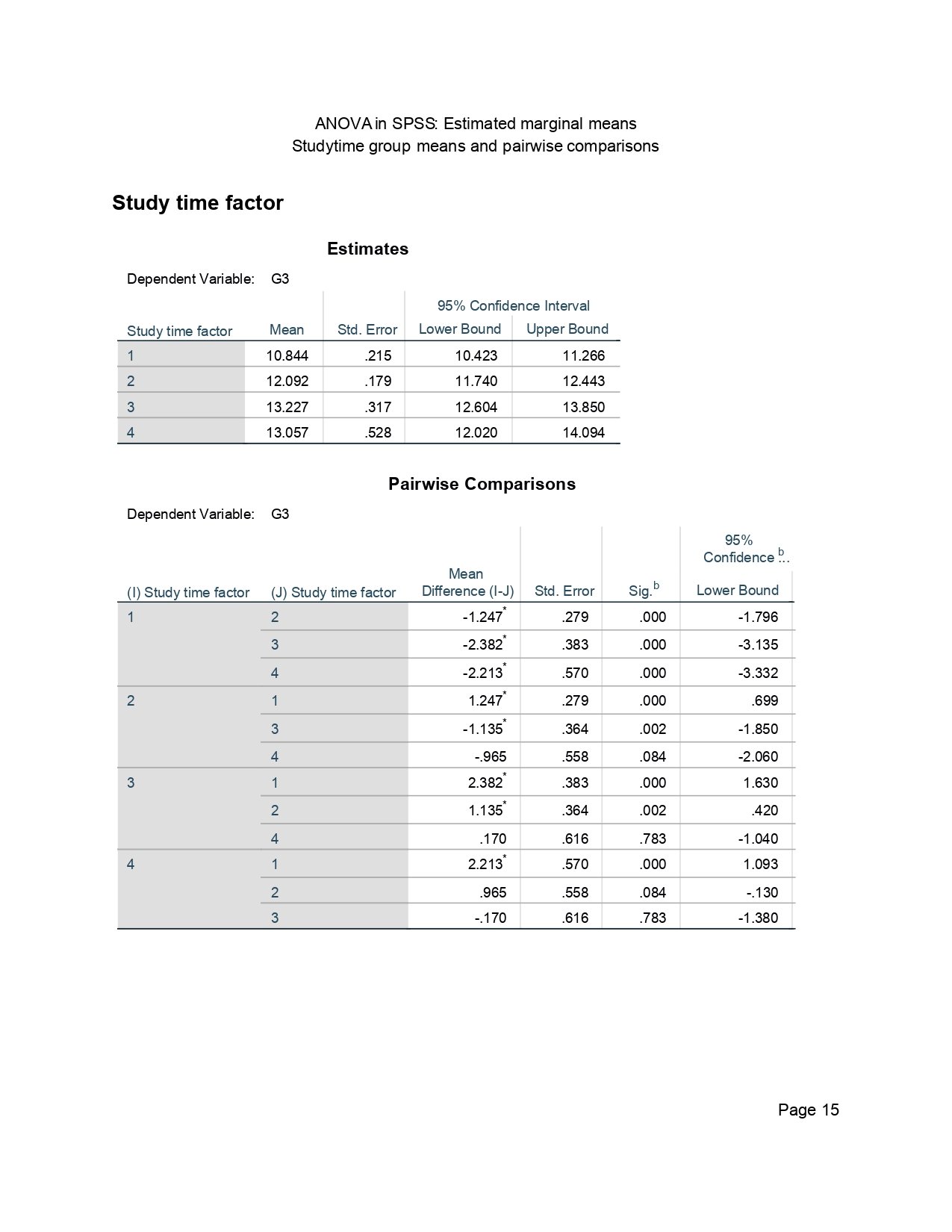
This page reports estimated marginal means for the studytime factor. The means are 10.844 for group 1, 12.092 for group 2, 13.227 for group 3 and 13.057 for group 4. These values match the descriptive means because the model has no covariate.
The pairwise comparisons show that group 1 is significantly lower than groups 2, 3 and 4. The mean difference for group 1 versus group 2 is -1.247, for group 1 versus group 3 is -2.382, and for group 1 versus group 4 is -2.213. All three comparisons are significant.
Group 2 versus group 3 is also significant, with a mean difference of -1.135 and p = .002 in the estimated marginal means output. Group 2 versus group 4 and group 3 versus group 4 are not significant. This gives the same practical pattern as the Tukey table: the lower studytime groups differ from the higher groups, but the highest two groups are not clearly separated.
SPSS Page 16: Pairwise Confidence Bounds and Univariate Test
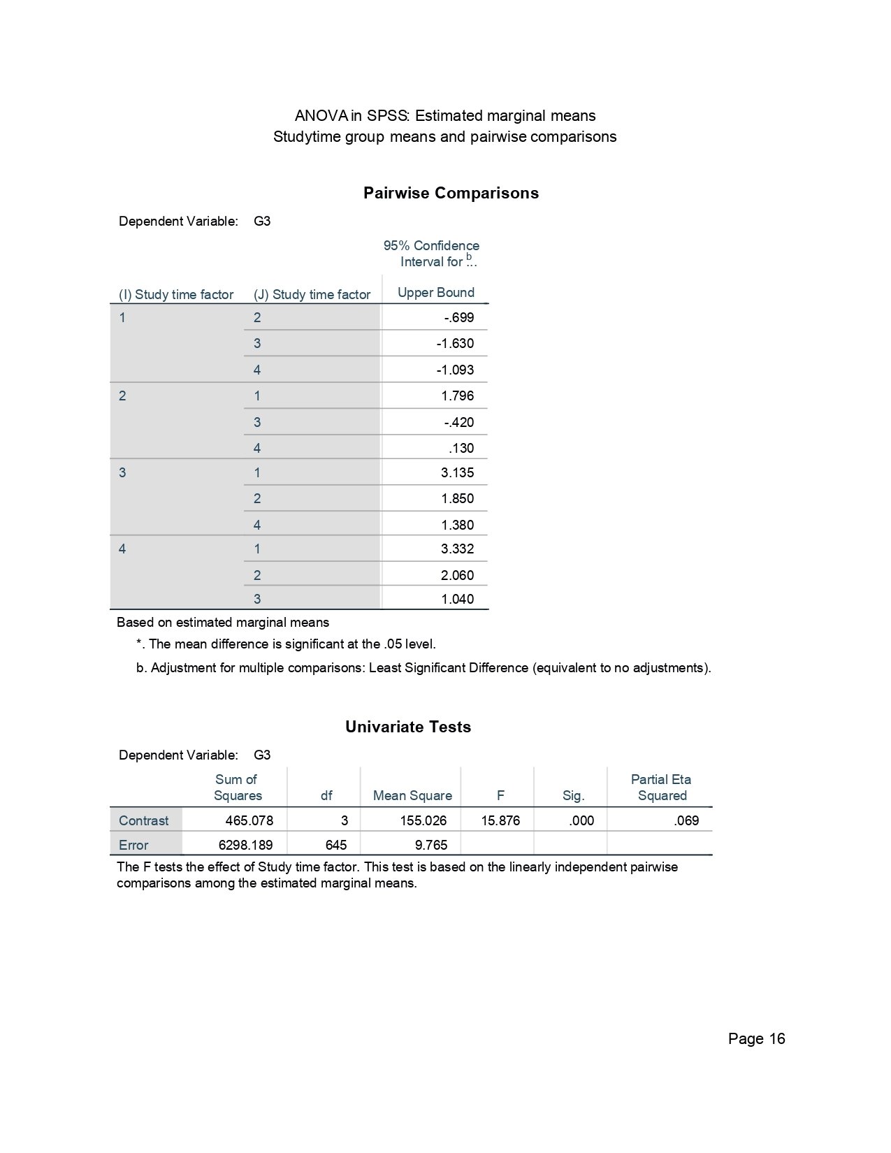
This page completes the pairwise comparison confidence intervals and shows the univariate test for the studytime factor. The univariate test again reports F = 15.876, Sig. = .000 and partial eta squared = .069.
The pairwise interval bounds confirm the same decision pattern. Significant comparisons have intervals that do not include zero, while non-significant comparisons include zero. For example, group 2 versus group 4 and group 3 versus group 4 include zero, so those pairwise differences are not statistically significant.
This page should be used to connect pairwise interpretation with the overall model result. The overall F test confirms that the factor matters, and the pairwise tables show where the differences are located.
SPSS Page 18: Residual Diagnostics Model Setup
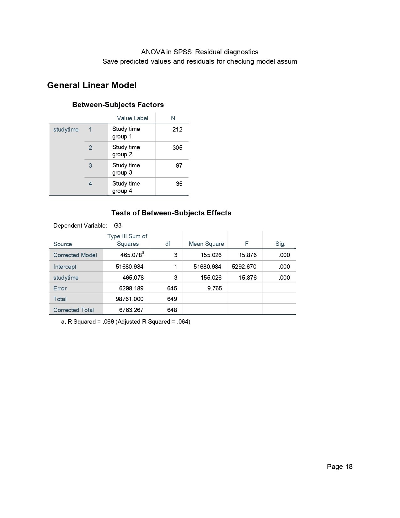
This page shows the GLM output used before saving predicted values and residuals. The same studytime result appears again: F = 15.876, p < .001, with SS effect = 465.078 and SS error = 6298.189.
The purpose of this page is diagnostic preparation. SPSS saves predicted values and residuals from this model so that the model assumptions can be checked through histograms, Q-Q plots, residual boxplots and residual-versus-predicted charts.
This page should be explained as the bridge between the ANOVA result and the assumption section. It confirms that the residual diagnostics are based on the same G3-by-studytime model.
SPSS Page 20: Residual Descriptives and Normality Tests
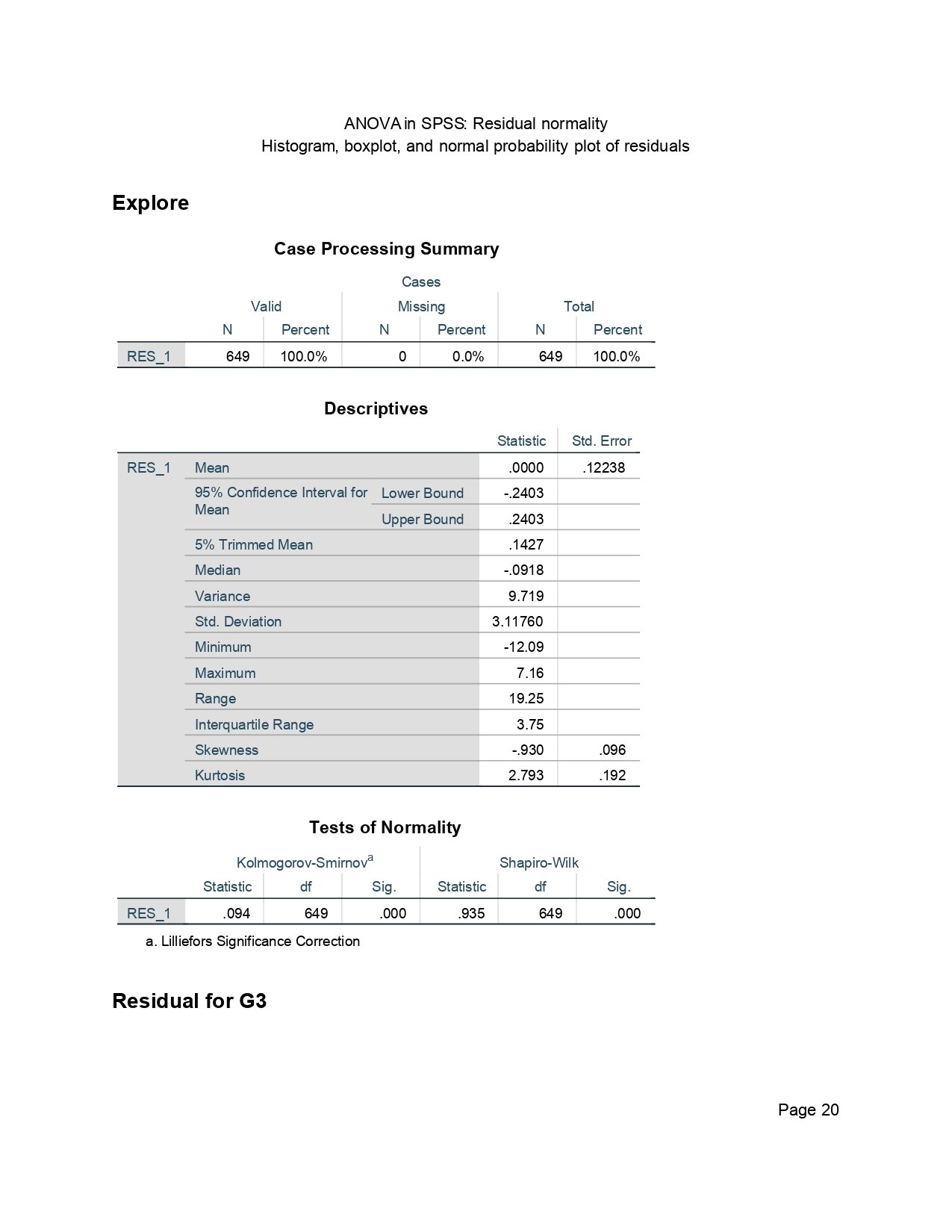
This residual page shows 649 valid residuals. The residual mean is essentially zero, and the residual standard deviation is 3.11760. The minimum residual is -12.09, and the maximum residual is 7.16, so the negative side of the residual distribution is more extreme than the positive side.
The residual skewness is -.930, and kurtosis is 2.793. This confirms the visible lower-tail pattern in the residual charts. The Kolmogorov-Smirnov and Shapiro-Wilk tests both show Sig. = .000, which should be written as p < .001.
Because the sample is large, formal normality tests can become significant even for visible but manageable departures. The correct interpretation is not that the ANOVA must automatically be abandoned. The better interpretation is that residuals are centered near zero but show lower-tail departures that should be discussed with the residual plots.
SPSS Page 21: Residual Histogram and Normal Q-Q Plot
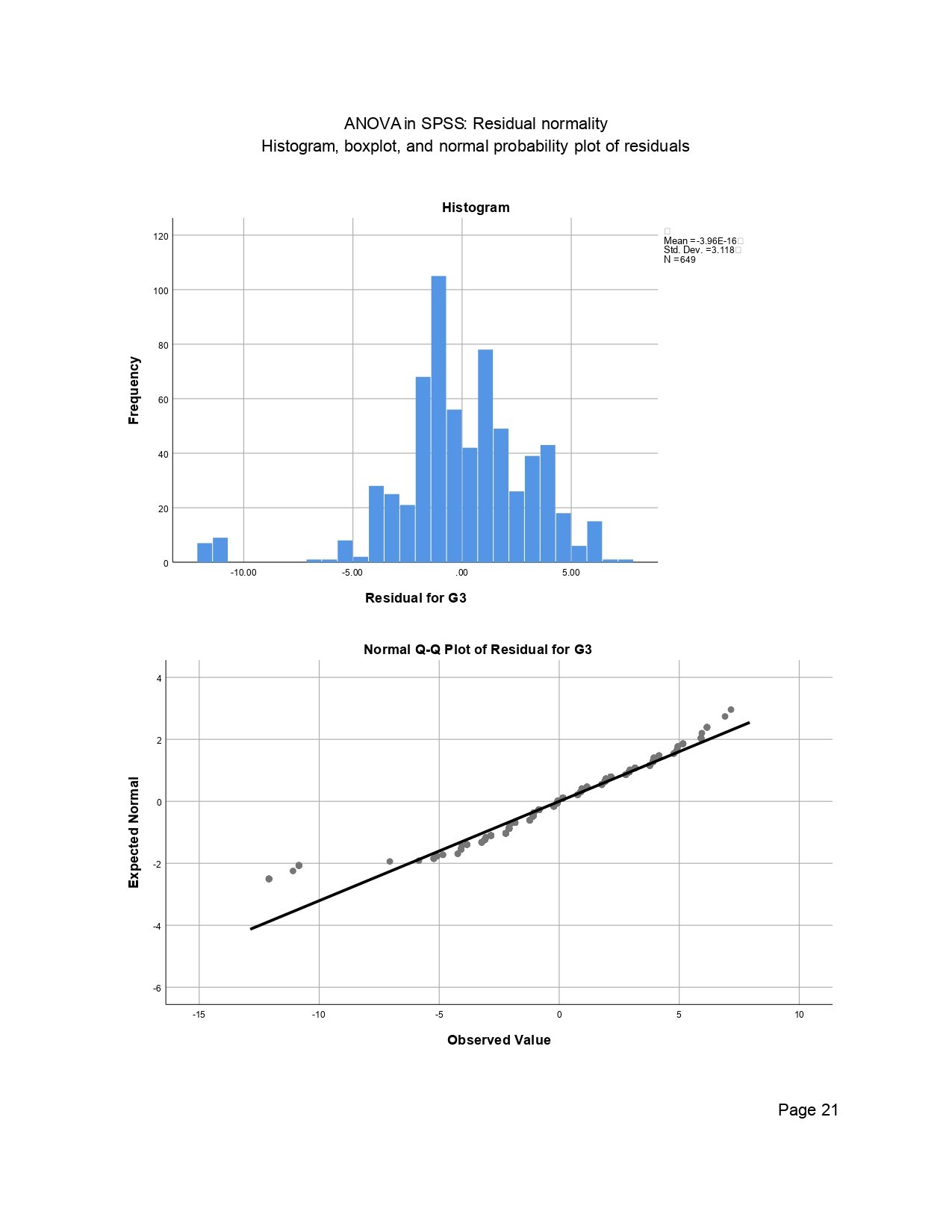
The histogram shows that most residuals are centered around zero, with the tallest bars near the middle of the distribution. The residual mean is essentially zero, and the standard deviation shown on the chart is about 3.118.
The histogram also shows a long negative tail, with a few residuals around -10 to -12. This means some students scored much lower than the studytime group mean predicted. The normal Q-Q plot shows that most central points follow the line, while the lower tail departs from the expected normal pattern.
This page supports a balanced assumption statement. The residual center is acceptable, but the lower tail contains unusual low-score cases. A correct report should mention this tail behavior instead of simply saying that residuals are perfectly normal.
SPSS Page 22: Detrended Q-Q Plot and Residual Boxplot
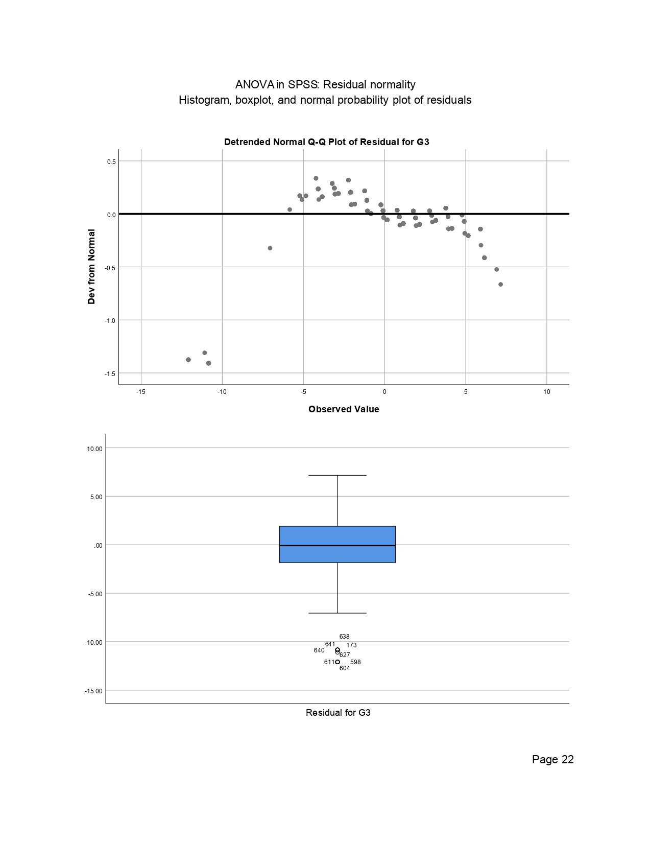
The detrended Q-Q plot shows deviations from normality more clearly. The central residuals stay relatively close to the zero line, but several lower-tail observations fall far below it. This matches the residual normality table and histogram.
The residual boxplot shows the residual median near zero and several labeled low outliers below the lower whisker. The labeled cases around the negative tail are the same type of observations that create the left-tail departure in the histogram and Q-Q plot.
This page should be used to describe residual diagnostics honestly. The model has a clear studytime effect and acceptable variance evidence, but residual normality is not perfect because of a small set of large negative residuals.
SPSS Page 24: Group Boxplot Descriptives, Part 1
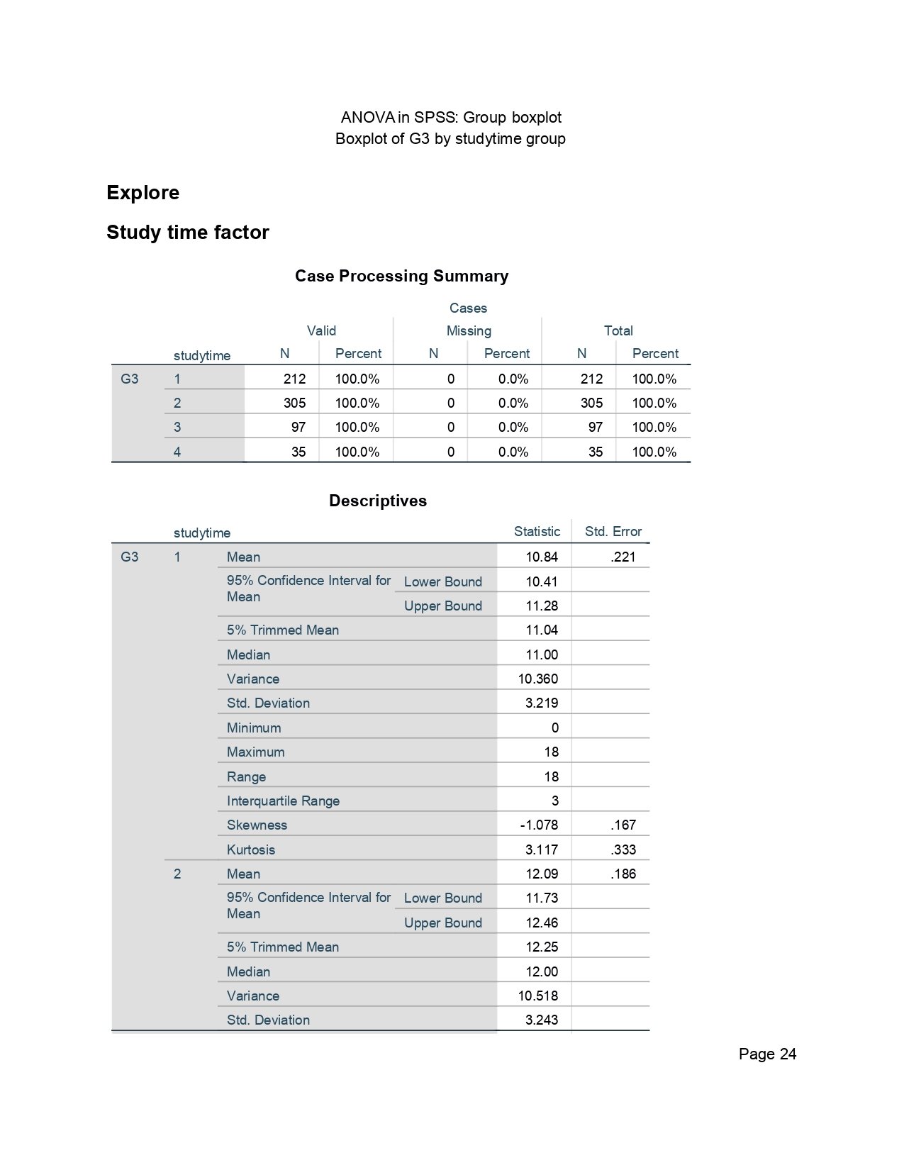
This page begins the group boxplot output. It shows the case processing summary by studytime group and the detailed descriptives for studytime group 1 and the start of group 2. Group 1 has a mean of 10.84, median of 11.00, variance of 10.360, standard deviation of 3.219, minimum of 0 and maximum of 18.
The group 1 skewness is -1.078, and kurtosis is 3.117. This confirms that the lowest studytime group contains a strong lower-tail pattern. Group 2 has a mean of 12.09, median of 12.00, variance of 10.518 and standard deviation of 3.243.
This page supports the later boxplot interpretation. The group mean difference is real, but the lower studytime groups also contain low-score cases that affect distribution shape and residual normality.
SPSS Page 25: Group Boxplot Descriptives, Part 2
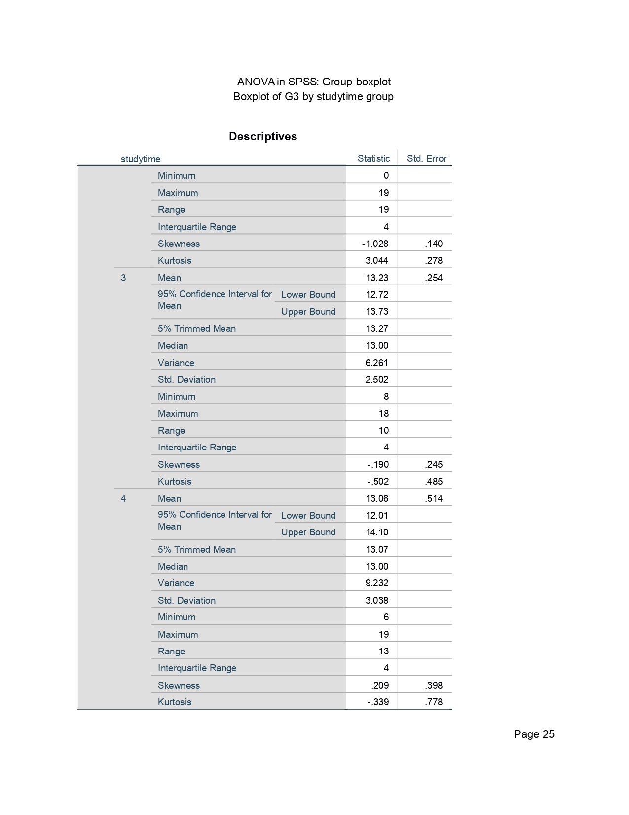
This page continues the group-specific descriptives. Studytime group 3 has a mean of 13.23, median of 13.00, variance of 6.261, standard deviation of 2.502, minimum of 8 and maximum of 18. Group 4 has a mean of 13.06, median of 13.00, variance of 9.232, standard deviation of 3.038, minimum of 6 and maximum of 19.
Group 3 has the smallest spread and no very low minimum value. Group 4 has a smaller sample size and wider uncertainty, but its center is close to group 3. This explains why groups 3 and 4 are not significantly different in the post hoc output.
This page should be used to connect the numerical descriptives with the boxplot. The highest studytime groups have higher centers, while group 1 and group 2 contain the lower-score observations that drive the strongest group differences.
SPSS Page 26: Boxplot of G3 by Studytime Group
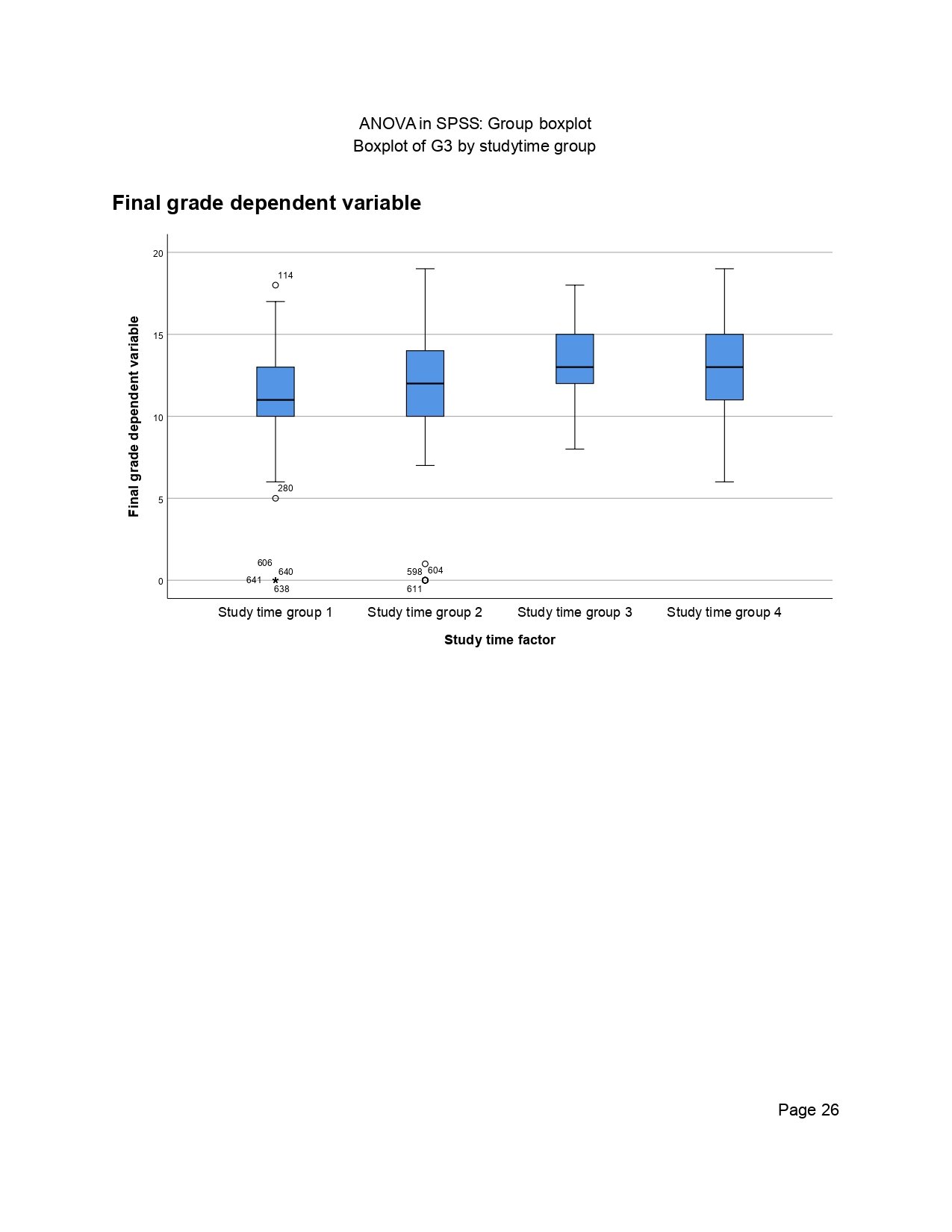
This boxplot shows the distribution of G3 across the four studytime groups. Group 1 has the lowest center, group 2 is higher, and groups 3 and 4 have higher medians. The visual pattern matches the descriptives and the means plot.
The chart also shows several low outliers in groups 1 and 2, including values near zero. Group 1 also has a high outlier near the upper part of the scale. Groups 3 and 4 show higher central scores and do not show the same extreme low-score pattern.
In reporting, this chart supports both the group difference and the diagnostic caution. The ANOVA result is significant, but the low-score outliers in the lower studytime groups should be acknowledged when discussing assumptions and residual normality.
SPSS Page 28: Means Plot for G3 Across Studytime Groups
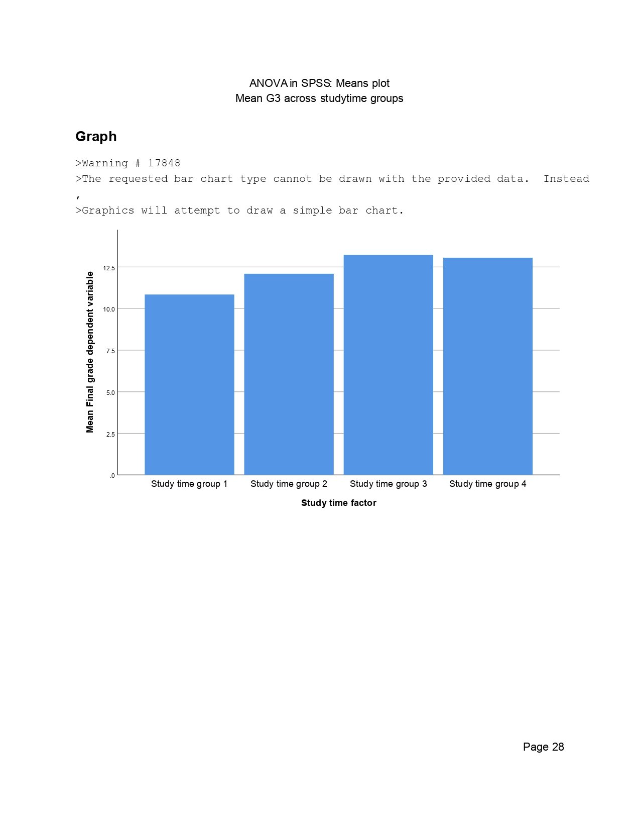
This means plot shows the same descriptive pattern in chart form. The mean G3 bar is lowest for studytime group 1, higher for group 2, highest for group 3 and slightly lower but still high for group 4.
The plot makes the direction of the ANOVA result easy to understand. The studytime effect is not random in direction; higher studytime groups generally have higher G3 scores than the lowest studytime group.
In a WordPress article, this plot is useful immediately after the ANOVA table or post hoc section. It explains the practical direction of the significant F result without requiring the reader to read every table value first.
SPSS Page 30: Residuals Versus Predicted Values
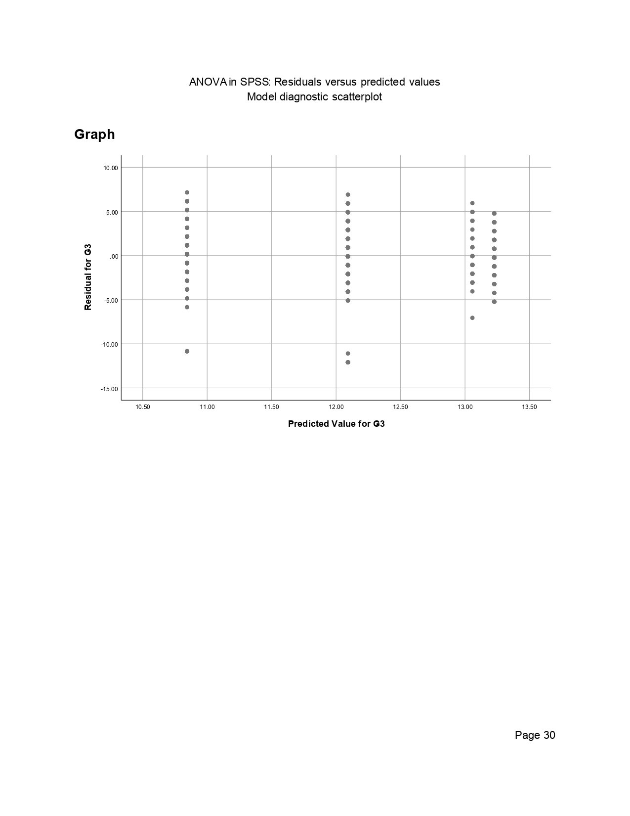
This chart plots residuals against predicted G3 values. The points appear in vertical bands because the one-way ANOVA model predicts group means. Each studytime group produces one predicted mean value, so the residuals stack vertically around those fitted values.
Most residuals are distributed around zero, but a few large negative residuals appear below -10. These cases represent students whose observed G3 was much lower than the studytime group mean predicted.
The plot does not show a strong funnel pattern across predicted values, which agrees with the non-significant Levene tests. The main diagnostic issue is not unequal spread across groups; it is the small number of large negative residuals.
SPSS Page 31: Residual Histogram with Normal Curve
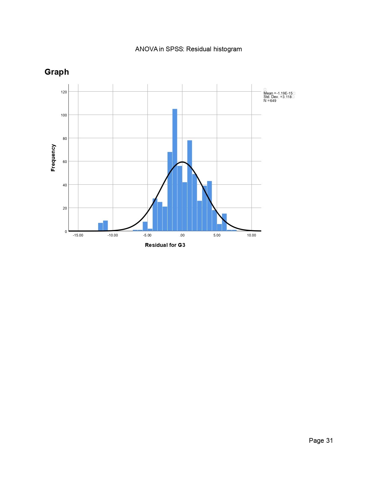
This residual histogram shows the residual distribution with a normal curve overlay. Most residuals fall near the center, and the mean shown on the chart is essentially zero. The standard deviation is about 3.118, with N = 649.
The left tail contains several low residual values around -10 to -12. This confirms the same diagnostic pattern shown in the Q-Q plot, detrended Q-Q plot, residual boxplot and residual-versus-predicted chart.
In reporting, this histogram supports the statement that residuals were centered around zero but showed lower-tail departures. This is the correct sample-style interpretation because it explains the actual chart result rather than giving a generic normality instruction.
SPSS Workflow for One-Way ANOVA
The SPSS workflow has three main parts: run the classical One-Way ANOVA, run GLM for effect size, and inspect residual diagnostics. The One-Way ANOVA output gives descriptives, Levene’s test, ANOVA table and Tukey HSD. The GLM output gives partial eta squared and estimated marginal means. The diagnostic output checks residual distribution and model assumptions.
| SPSS Step | Menu Path | Purpose | Output to Read |
|---|---|---|---|
| Run classical ANOVA | Analyze > Compare Means > One-Way ANOVA | Compare G3 means across studytime groups. | Descriptives, Levene test, ANOVA table and Tukey HSD. |
| Set dependent variable | Move G3 to Dependent List | Define the numeric outcome. | G3 descriptive and ANOVA output. |
| Set factor | Move studytime to Factor | Define the grouping variable. | Studytime group rows and comparisons. |
| Request post hoc | Post Hoc > Tukey | Find which group pairs differ. | Multiple Comparisons and homogeneous subsets. |
| Request homogeneity | Options > Homogeneity of variance test | Check equal variance assumption. | Levene’s test. |
| Run GLM | Analyze > General Linear Model > Univariate | Get partial eta squared and estimated marginal means. | Tests of Between-Subjects Effects. |
| Save residuals | GLM Save options or syntax | Create residual and predicted variables. | Residual histogram, Q-Q plot and residual scatterplot. |
SPSS, R, Python and Excel Workflows for ANOVA
The same ANOVA model can be reproduced in SPSS, R, Python and Excel. This article focuses on SPSS, but the comparison table helps readers translate the same G3-by-studytime model across common software.
SPSS Workflow
| Step | SPSS Menu | Purpose |
|---|---|---|
| Open data | File > Open > Data | Load G3 and studytime variables. |
| Run ANOVA | Analyze > Compare Means > One-Way ANOVA | Compare G3 means across groups. |
| Request descriptives | Options > Descriptive | Get group means and confidence intervals. |
| Request homogeneity | Options > Homogeneity of variance test | Get Levene’s test. |
| Request post hoc | Post Hoc > Tukey | Identify significant group pairs. |
| Run GLM | Analyze > General Linear Model > Univariate | Get partial eta squared. |
R Workflow
| Step | R Code | Purpose |
|---|---|---|
| Read data | read.csv("dataset.csv") | Load dataset. |
| Set factor | df$studytime <- as.factor(df$studytime) | Prepare group variable. |
| Run ANOVA | aov(G3 ~ studytime, data=df) | Fit one-way ANOVA. |
| Read result | summary(model) | Get F statistic and p value. |
| Post hoc | TukeyHSD(model) | Compare group pairs. |
Python Workflow
| Step | Python Code | Purpose |
|---|---|---|
| Read data | pd.read_csv("dataset.csv") | Load dataset. |
| Run ANOVA | ols("G3 ~ C(studytime)", data=df) | Fit one-way ANOVA model. |
| ANOVA table | sm.stats.anova_lm(model, typ=2) | Get SS, df, F and p. |
| Post hoc | pairwise_tukeyhsd() | Run Tukey HSD. |
| Effect size | eta_sq = ss_between / ss_total | Calculate effect size. |
Excel Workflow
| Step | Excel Tool or Formula | Purpose |
|---|---|---|
| Arrange groups | Place each studytime group in a separate column | Prepare data for ANOVA ToolPak. |
| Run ANOVA | Data Analysis ToolPak > ANOVA: Single Factor | Get ANOVA table. |
| Calculate eta squared | =SS_Between/SS_Total | Calculate effect size. |
| Calculate residuals | =Observed - GroupMean | Check model errors. |
| Create plots | Insert > Chart | Visualize means and residuals. |
Code Blocks for ANOVA in SPSS
SPSS Syntax: Classical One-Way ANOVA with Tukey HSD
* ANOVA in SPSS: One-way ANOVA with descriptives, homogeneity and Tukey post hoc.
* Dependent variable: G3.
* Factor: studytime.

TITLE "ANOVA in SPSS: One-Way ANOVA for G3 by Studytime".

ONEWAY G3 BY studytime
  /STATISTICS DESCRIPTIVES HOMOGENEITY
  /POSTHOC = TUKEY ALPHA(.05)
  /MISSING ANALYSIS.
SPSS Syntax: GLM with Partial Eta Squared and Estimated Means
* GLM version for partial eta squared and estimated marginal means.

UNIANOVA G3 BY studytime
  /METHOD = SSTYPE(3)
  /INTERCEPT = INCLUDE
  /PRINT = DESCRIPTIVE ETASQ HOMOGENEITY PARAMETER
  /EMMEANS = TABLES(studytime) COMPARE ADJ(LSD)
  /CRITERIA = ALPHA(.05)
  /DESIGN = studytime.
SPSS Syntax: Save Predicted Values and Residuals
* Save predicted values and residuals for assumption checks.

UNIANOVA G3 BY studytime
  /METHOD = SSTYPE(3)
  /INTERCEPT = INCLUDE
  /PRINT = DESCRIPTIVE ETASQ HOMOGENEITY
  /SAVE = PRED RESID
  /CRITERIA = ALPHA(.05)
  /DESIGN = studytime.

EXAMINE VARIABLES = RES_1
  /PLOT BOXPLOT HISTOGRAM NPPLOT
  /STATISTICS DESCRIPTIVES
  /CINTERVAL 95
  /MISSING LISTWISE
  /NOTOTAL.
SPSS Syntax: Export Output to PDF
* Export the visible SPSS output to PDF.

OUTPUT EXPORT
  /CONTENTS EXPORT = VISIBLE
  /PDF DOCUMENTFILE = "ANOVA-in-SPSS-Output.pdf".
R Code for the Same ANOVA
df <- read.csv("dataset.csv")

df$G3 <- as.numeric(df$G3)
df$studytime <- as.factor(df$studytime)

df_model <- na.omit(df[, c("G3", "studytime")])

model <- aov(G3 ~ studytime, data = df_model)

summary(model)
TukeyHSD(model)

aggregate(G3 ~ studytime, data = df_model, FUN = mean)
Python Code for the Same ANOVA
import pandas as pd
import statsmodels.api as sm
from statsmodels.formula.api import ols
from statsmodels.stats.multicomp import pairwise_tukeyhsd

df = pd.read_csv("dataset.csv")

df["G3"] = pd.to_numeric(df["G3"], errors="coerce")
df["studytime"] = df["studytime"].astype("category")

df_model = df.dropna(subset=["G3", "studytime"])

model = ols("G3 ~ C(studytime)", data=df_model).fit()
anova_table = sm.stats.anova_lm(model, typ=2)

print(anova_table)
print(df_model.groupby("studytime")["G3"].agg(["count", "mean", "std", "var"]))

tukey = pairwise_tukeyhsd(
    endog=df_model["G3"],
    groups=df_model["studytime"],
    alpha=0.05
)

print(tukey)
Excel Formulas for SPSS ANOVA Values
Group mean:
=AVERAGE(group_range)

Group standard deviation:
=STDEV.S(group_range)

Total sum of squares:
=SS_Between + SS_Within

Mean square between:
=SS_Between / df_Between

Mean square within:
=SS_Within / df_Within

F statistic:
=MS_Between / MS_Within

Eta squared:
=SS_Between / SS_Total

Partial eta squared:
=SS_Between / (SS_Between + SS_Within)
APA Reporting Wording
When reporting ANOVA in SPSS, include the dependent variable, grouping factor, group means, homogeneity result, F statistic, degrees of freedom, p value, effect size and post hoc comparison results. SPSS output should be translated into reporting language rather than copied as screenshots only.
APA-style report: A one-way ANOVA was conducted in SPSS to compare G3 final grade across four studytime groups. Mean G3 increased from studytime group 1 (M = 10.84, SD = 3.219) to group 2 (M = 12.09, SD = 3.243), group 3 (M = 13.23, SD = 2.502) and group 4 (M = 13.06, SD = 3.038). Levene’s test was not significant based on the mean, p = .400, supporting homogeneity of variance. The ANOVA was significant, F(3, 645) = 15.876, p < .001, partial η² = .069. Tukey HSD showed that group 1 was significantly lower than groups 2, 3 and 4, and group 2 was significantly lower than group 3.
Short reporting version: The SPSS one-way ANOVA showed a significant studytime effect on G3, F(3, 645) = 15.876, p < .001, partial η² = .069. Tukey HSD indicated that the lowest studytime group differed significantly from the higher studytime groups.
Common Mistakes
| Mistake | Why It Is Wrong | Correct Practice |
|---|---|---|
| Writing p = .000 | SPSS displays .000 when the value is very small, not exactly zero. | Write p < .001. |
| Reporting only the ANOVA table | The ANOVA table does not show which groups differ. | Add Tukey HSD or planned comparisons. |
| Ignoring Levene’s test | Ordinary ANOVA assumes similar group variances. | Report Levene’s test before the F test. |
| Ignoring effect size | A significant p value does not show practical magnitude. | Report partial eta squared, eta squared or omega squared. |
| Interpreting all four groups as separate | Post hoc output shows which groups are actually different. | Use Tukey and homogeneous subsets to summarize the pattern. |
| Ignoring residual diagnostics | ANOVA assumptions still need review. | Check residual histogram, Q-Q plot and residual scatterplot. |
When to Use ANOVA in SPSS
Use ANOVA in SPSS when you need to compare a numeric outcome across three or more independent groups. In this example, one-way ANOVA is appropriate because G3 is numeric and studytime has four independent groups.
| Research Situation | SPSS Method | Example |
|---|---|---|
| One numeric outcome and one group factor | One-Way ANOVA | G3 by studytime. |
| One numeric outcome and two factors | Univariate GLM | G3 by school and studytime. |
| Group comparison with a covariate | ANCOVA using GLM | G3 by school adjusted for G2. |
| Repeated measurements on the same subjects | Repeated Measures ANOVA | Scores across multiple time points. |
| Only two independent groups | Independent Samples T Test | GP versus MS school comparison. |
For related mean-comparison tutorials, see ANOVA in Python, ANOVA in R, ANOVA Effect Size, ANOVA Assumptions, T Test vs ANOVA, ANCOVA, Two Sample T Test, Independent Samples T Test, and Welch’s T Test.
Downloads and Resources for ANOVA in SPSS
Use these resources to reproduce the ANOVA in SPSS workflow. The PDF link contains the exported SPSS output used in this guide. Replace placeholder links with final hosted dataset, SPSS syntax, R script, Python script and Excel workbook URLs after uploading them to WordPress Media Library.
Download Dataset
Practice dataset with G3 and studytime variables.
Download ANOVA in SPSS Output PDF
Complete SPSS output PDF with descriptives, Levene test, ANOVA table, post hoc output, effect size and diagnostics.
Download SPSS Syntax
SPSS syntax for one-way ANOVA, GLM effect size, residual diagnostics and PDF export.
Download R, Python and Excel Files
Validation scripts and spreadsheet formulas for the same ANOVA model.
FAQs About ANOVA in SPSS
What is ANOVA in SPSS?
ANOVA in SPSS is a mean-comparison procedure used to test whether three or more group means are statistically different.
How do I run one-way ANOVA in SPSS?
Use Analyze > Compare Means > One-Way ANOVA. Put the numeric outcome in Dependent List and the grouping variable in Factor.
What is the dependent variable in this SPSS ANOVA example?
The dependent variable is G3 final grade.
What is the factor in this SPSS ANOVA example?
The factor is studytime, which has four groups.
How do I interpret the SPSS ANOVA table?
Read the F statistic, degrees of freedom and Sig. value. In this output, F(3,645) = 15.876, p < .001, so the group means differ significantly.
What does Levene’s test show in this SPSS output?
Levene’s test is not significant. The mean-based p value is .400, so the homogeneity of variance assumption is supported.
What does Tukey HSD show in this SPSS ANOVA output?
Tukey HSD shows that studytime group 1 differs significantly from groups 2, 3 and 4, and group 2 differs significantly from group 3.
What is partial eta squared in this SPSS ANOVA?
The GLM output reports partial eta squared = .069 for studytime, meaning studytime explains about 6.9% of the effect-plus-error variation in G3.
How should SPSS Sig. = .000 be reported?
SPSS Sig. = .000 should be reported as p < .001, not p = .000.
What is the APA wording for this SPSS ANOVA?
A concise report is: A one-way ANOVA in SPSS showed a significant studytime effect on G3, F(3,645) = 15.876, p < .001, partial η² = .069.

