
.abx-article{–ink:#102238;–muted:#52657a;–line:#dce5ed;–paper:#fff;–soft:#f4f8fb;–navy:#092a45;–teal:#0d7774;–cyan:#dff7f6;–amber:#f4a340;–amber-soft:#fff4df;–red:#a83232;–red-soft:#fff0f0;–green:#176b47;–green-soft:#e9f8f0;–violet:#6654b8;–violet-soft:#f0edff;–shadow:0 16px 45px rgba(18,44,67,.10);font-family:Inter,ui-sans-serif,system-ui,-apple-system,BlinkMacSystemFont,”Segoe UI”,Arial,sans-serif;color:var(–ink);line-height:1.72;width:auto;max-width:none!important;margin-left:calc(50% – 50vw + 12px)!important;margin-right:calc(50% – 50vw + 12px)!important;margin-top:0!important;margin-bottom:0!important;background:var(–paper);font-size:17px;overflow-x:clip}
.abx-article *{box-sizing:border-box}.abx-article a{color:#075f72;text-decoration-thickness:1px;text-underline-offset:3px}.abx-article a:hover{color:#043f4c}.abx-shell{width:100%;max-width:1480px;margin:0 auto;padding:clamp(18px,2.8vw,42px)}.abx-hero{position:relative;overflow:hidden;border-radius:28px;background:linear-gradient(132deg,#07263f 0%,#0b4b61 55%,#0a7770 100%);color:#fff;padding:clamp(28px,6vw,68px);box-shadow:var(–shadow)}.abx-hero:before{content:””;position:absolute;right:-90px;top:-120px;width:360px;height:360px;border-radius:50%;background:rgba(255,255,255,.07)}.abx-hero:after{content:””;position:absolute;left:-110px;bottom:-180px;width:390px;height:390px;border-radius:50%;background:rgba(244,163,64,.10)}.abx-hero>*{position:relative;z-index:1}.abx-kicker{display:inline-flex;align-items:center;gap:9px;padding:7px 12px;border:1px solid rgba(255,255,255,.25);border-radius:999px;background:rgba(255,255,255,.09);font-size:.78rem;font-weight:800;letter-spacing:.08em;text-transform:uppercase}.abx-kicker i{width:9px;height:9px;border-radius:50%;background:#ffbd62;box-shadow:0 0 0 5px rgba(255,189,98,.16)}.abx-hero h1{font-size:clamp(2.15rem,5.2vw,4.65rem);line-height:1.04;letter-spacing:-.045em;margin:22px 0 18px;max-width:1000px;color:#fff}.abx-hero .abx-lead{font-size:clamp(1.05rem,2vw,1.34rem);max-width:900px;color:#e9f7fb;margin:0}.abx-badges{display:flex;flex-wrap:wrap;gap:10px;margin-top:25px}.abx-badge{padding:8px 12px;border-radius:999px;background:rgba(255,255,255,.11);border:1px solid rgba(255,255,255,.19);font-size:.84rem;font-weight:750}.abx-hero-result{margin-top:28px;display:grid;grid-template-columns:repeat(4,minmax(0,1fr));gap:12px}.abx-hero-metric{background:rgba(255,255,255,.10);border:1px solid rgba(255,255,255,.16);border-radius:16px;padding:14px}.abx-hero-metric span{display:block;color:#cdeaf0;font-size:.78rem;text-transform:uppercase;letter-spacing:.05em;font-weight:800}.abx-hero-metric strong{display:block;margin-top:4px;font-size:1.28rem;color:#fff}.abx-ad{display:flex;align-items:center;justify-content:center;min-height:96px;margin:26px 0;border:1px dashed #b8c6d1;border-radius:18px;background:#f8fafc;color:#718096;font-size:.78rem;letter-spacing:.14em;text-transform:uppercase}.abx-quick{display:grid;grid-template-columns:1.35fr .65fr;gap:20px;margin:28px 0}.abx-card{min-width:0;max-width:100%;border:1px solid var(–line);border-radius:22px;background:#fff;box-shadow:0 10px 30px rgba(21,48,70,.06);padding:clamp(19px,3vw,30px)}.abx-card h2,.abx-card h3{margin-top:0}.abx-answer{background:linear-gradient(145deg,#f2fbfa,#fff);border-color:#bfe5e2}.abx-answer .abx-verdict{display:inline-flex;align-items:center;gap:9px;padding:8px 12px;border-radius:999px;background:var(–green-soft);color:var(–green);font-weight:850;font-size:.84rem}.abx-answer .abx-verdict:before{content:”✓”;display:grid;place-items:center;width:22px;height:22px;border-radius:50%;background:var(–green);color:#fff}.abx-answer h2{font-size:clamp(1.55rem,3vw,2.25rem);line-height:1.15;margin:15px 0 10px}.abx-mini-table{display:grid;gap:10px}.abx-mini-row{display:flex;justify-content:space-between;gap:20px;padding:11px 0;border-bottom:1px solid var(–line)}.abx-mini-row:last-child{border-bottom:0}.abx-mini-row span{color:var(–muted)}.abx-mini-row strong{text-align:right}.abx-toc{margin:26px 0;border-radius:22px;background:var(–navy);color:#fff;padding:24px}.abx-toc h2{color:#fff;margin:0 0 14px;font-size:1.2rem}.abx-toc-grid{display:grid;grid-template-columns:repeat(3,minmax(0,1fr));gap:8px 20px}.abx-toc a{color:#d9f6f5;text-decoration:none;padding:7px 0;display:block;border-bottom:1px solid rgba(255,255,255,.12)}.abx-toc a:hover{color:#fff}.abx-section{scroll-margin-top:24px;margin:54px 0}.abx-section-head{display:grid;grid-template-columns:auto 1fr;align-items:start;gap:14px;margin-bottom:20px}.abx-num{width:42px;height:42px;border-radius:13px;background:var(–navy);color:#fff;display:grid;place-items:center;font-weight:900}.abx-section-head h2{margin:0;font-size:clamp(1.65rem,3.4vw,2.65rem);line-height:1.15;letter-spacing:-.025em}.abx-section-head p{grid-column:2;margin:5px 0 0;color:var(–muted);max-width:920px}.abx-grid-2{display:grid;grid-template-columns:repeat(2,minmax(0,1fr));gap:20px}.abx-grid-2>*,.abx-grid-3>*,.abx-grid-4>*,.abx-chart-grid>*,.abx-downloads>*,.abx-related>*,.abx-quick>*{min-width:0}.abx-grid-3{display:grid;grid-template-columns:repeat(3,minmax(0,1fr));gap:18px}.abx-grid-4{display:grid;grid-template-columns:repeat(4,minmax(0,1fr));gap:14px}.abx-callout{border-radius:18px;padding:18px 20px;border-left:5px solid var(–teal);background:var(–cyan);margin:20px 0}.abx-callout strong{color:#084f4c}.abx-warning{border-left-color:var(–red);background:var(–red-soft)}.abx-warning strong{color:var(–red)}.abx-note{border-left-color:var(–amber);background:var(–amber-soft)}.abx-note strong{color:#875311}.abx-formula{border:1px solid #cbd8e3;background:linear-gradient(180deg,#fff,#f7fafc);border-radius:20px;padding:22px;margin:18px 0;text-align:center;overflow:visible}.abx-formula .eq{font-family:”Cambria Math”,”Times New Roman”,serif;font-size:clamp(1.08rem,2.2vw,1.5rem);white-space:normal;overflow-wrap:anywhere;word-break:normal;line-height:1.55}.abx-formula p{margin:8px auto 0;color:var(–muted);max-width:850px;text-align:left;font-size:.94rem}.abx-pill-list{display:flex;flex-wrap:wrap;gap:10px;margin:15px 0}.abx-pill{background:var(–soft);border:1px solid var(–line);border-radius:999px;padding:8px 12px;font-weight:750;font-size:.88rem}.abx-flow{display:grid;grid-template-columns:repeat(5,minmax(0,1fr));gap:10px;counter-reset:flow}.abx-step{position:relative;padding:18px 14px 16px;border:1px solid var(–line);border-radius:18px;background:#fff;min-height:148px}.abx-step:before{counter-increment:flow;content:counter(flow);display:grid;place-items:center;width:30px;height:30px;border-radius:10px;background:var(–teal);color:#fff;font-weight:900;margin-bottom:10px}.abx-step h3{font-size:1rem;margin:0 0 6px}.abx-step p{font-size:.9rem;color:var(–muted);margin:0}.abx-table-wrap{min-width:0;max-width:100%;overflow-x:auto;border:1px solid var(–line);border-radius:18px;background:#fff}.abx-table{width:100%;border-collapse:collapse;min-width:720px}.abx-table.abx-compact{min-width:0}.abx-table th{background:var(–navy);color:#fff;text-align:left;padding:13px 14px;font-size:.85rem;letter-spacing:.02em}.abx-table td{padding:13px 14px;border-bottom:1px solid var(–line);vertical-align:top}.abx-table tbody tr:nth-child(even){background:#f8fafc}.abx-table tbody tr:last-child td{border-bottom:0}.abx-stat-grid{display:grid;grid-template-columns:repeat(4,minmax(0,1fr));gap:12px;margin:16px 0}.abx-stat{border:1px solid var(–line);border-radius:16px;padding:16px;background:#fff}.abx-stat span{display:block;color:var(–muted);font-size:.78rem;font-weight:800;text-transform:uppercase;letter-spacing:.05em}.abx-stat strong{display:block;font-size:1.34rem;margin-top:4px}.abx-stat small{display:block;color:var(–muted);margin-top:4px}.abx-result-panel{border-radius:22px;background:linear-gradient(145deg,#082c47,#0b5966);color:#fff;padding:26px}.abx-result-panel h3{color:#fff;margin-top:0;font-size:1.45rem}.abx-result-panel p{color:#e5f6f7}.abx-result-panel .abx-result-big{font-size:clamp(2rem,5vw,3.7rem);line-height:1;font-weight:950;color:#fff;margin:10px 0}.abx-result-panel .abx-result-tag{display:inline-block;padding:8px 12px;border-radius:999px;background:rgba(255,255,255,.12);border:1px solid rgba(255,255,255,.18);font-weight:800}.abx-figure{min-width:0;max-width:100%;margin:0;border:1px solid var(–line);border-radius:22px;overflow:hidden;background:#fff;box-shadow:0 10px 30px rgba(21,48,70,.06)}.abx-figure img{display:block;width:100%;height:auto;background:#f3f6f8}.abx-figure figcaption{padding:18px 20px}.abx-figure h3{font-size:1.08rem;margin:0 0 6px}.abx-figure p{margin:0;color:var(–muted);font-size:.94rem}.abx-chart-grid{display:grid;grid-template-columns:repeat(2,minmax(0,1fr));gap:20px}.abx-chart-grid .abx-wide{grid-column:1/-1}.abx-code{min-width:0;max-width:100%;position:relative;background:#071d2d;color:#e6f2f7;border-radius:18px;overflow:auto;padding:20px;margin:16px 0;box-shadow:inset 0 0 0 1px rgba(255,255,255,.07)}.abx-code code{display:block;white-space:pre;min-width:max-content;font-family:”SFMono-Regular”,Consolas,”Liberation Mono”,monospace;font-size:.88rem;line-height:1.65}.abx-code-label{display:inline-block;margin-bottom:8px;color:#7ee7db;font-size:.76rem;font-weight:900;letter-spacing:.08em;text-transform:uppercase}.abx-downloads{display:grid;grid-template-columns:repeat(4,minmax(0,1fr));gap:14px}.abx-download{display:flex;flex-direction:column;min-height:190px;padding:20px;border-radius:20px;border:1px solid var(–line);background:#fff;text-decoration:none!important;color:var(–ink)!important;box-shadow:0 10px 30px rgba(21,48,70,.06);transition:.2s transform,.2s box-shadow}.abx-download:hover{transform:translateY(-3px);box-shadow:0 16px 38px rgba(21,48,70,.12)}.abx-file-icon{width:46px;height:46px;border-radius:14px;display:grid;place-items:center;background:var(–violet-soft);color:var(–violet);font-weight:950;margin-bottom:16px}.abx-download strong{font-size:1.05rem}.abx-download span{color:var(–muted);font-size:.88rem;margin-top:6px}.abx-download em{margin-top:auto;padding-top:16px;color:#075f72;font-style:normal;font-weight:850}.abx-checks{display:grid;gap:10px}.abx-check{position:relative;padding:13px 14px 13px 44px;border:1px solid var(–line);border-radius:15px;background:#fff}.abx-check:before{content:”✓”;position:absolute;left:14px;top:13px;width:22px;height:22px;border-radius:50%;display:grid;place-items:center;background:var(–green-soft);color:var(–green);font-weight:950}.abx-faq details{border:1px solid var(–line);border-radius:17px;background:#fff;margin:11px 0;overflow:hidden}.abx-faq summary{cursor:pointer;font-weight:850;padding:17px 20px;list-style:none}.abx-faq summary::-webkit-details-marker{display:none}.abx-faq summary:after{content:”+”;float:right;color:var(–teal);font-size:1.4rem;line-height:1}.abx-faq details[open] summary:after{content:”−”}.abx-faq .abx-faq-answer{padding:0 20px 18px;color:var(–muted)}.abx-related{display:grid;grid-template-columns:repeat(3,minmax(0,1fr));gap:12px}.abx-related a{display:block;border:1px solid var(–line);border-radius:15px;padding:14px 16px;background:#fff;text-decoration:none;font-weight:800}.abx-footer-note{border-radius:22px;background:var(–soft);border:1px solid var(–line);padding:22px;color:var(–muted)}.abx-back{display:inline-flex;align-items:center;gap:8px;border-radius:999px;background:var(–navy);color:#fff!important;text-decoration:none!important;padding:11px 16px;font-weight:850;margin-top:18px}.abx-sr{position:absolute!important;width:1px!important;height:1px!important;padding:0!important;margin:-1px!important;overflow:hidden!important;clip:rect(0,0,0,0)!important;white-space:nowrap!important;border:0!important}
@media(max-width:960px){.abx-hero-result,.abx-grid-4,.abx-stat-grid,.abx-downloads{grid-template-columns:repeat(2,minmax(0,1fr))}.abx-toc-grid,.abx-grid-3,.abx-related{grid-template-columns:repeat(2,minmax(0,1fr))}.abx-flow{grid-template-columns:repeat(2,minmax(0,1fr))}.abx-flow .abx-step:last-child{grid-column:1/-1}.abx-quick{grid-template-columns:1fr}}
@media(max-width:680px){.abx-article{font-size:16px;margin-left:calc(50% – 50vw + 6px)!important;margin-right:calc(50% – 50vw + 6px)!important}.abx-shell{padding:12px}.abx-hero{border-radius:20px;padding:26px 20px}.abx-hero h1{font-size:2.2rem}.abx-hero-result,.abx-grid-2,.abx-grid-3,.abx-grid-4,.abx-stat-grid,.abx-downloads,.abx-chart-grid,.abx-toc-grid,.abx-related,.abx-flow{grid-template-columns:1fr}.abx-chart-grid .abx-wide,.abx-flow .abx-step:last-child{grid-column:auto}.abx-card{border-radius:18px;padding:18px}.abx-section{margin:42px 0}.abx-section-head{grid-template-columns:36px 1fr;gap:11px}.abx-num{width:36px;height:36px}.abx-section-head p{grid-column:1/-1}.abx-table{min-width:650px}.abx-formula{padding:18px 12px;text-align:left}.abx-formula .eq{font-size:1.05rem}.abx-mini-row{align-items:flex-start;flex-direction:column;gap:2px}.abx-mini-row strong{text-align:left}}
.abx-seo-context{font-size:1.02rem;color:#31475d;margin:-5px 0 20px;max-width:1180px}
.abx-model{display:grid;grid-template-columns:1.05fr .95fr;gap:20px;align-items:stretch}
.abx-model .abx-card{height:100%}
.abx-hypothesis{border:1px solid var(–line);border-radius:18px;padding:20px;background:#fff}
.abx-hypothesis h3{margin:0 0 10px}
.abx-direction{display:grid;grid-template-columns:repeat(3,minmax(0,1fr));gap:12px;margin:16px 0}
.abx-direction>div{border:1px solid var(–line);border-radius:16px;padding:16px;background:var(–soft)}
.abx-keyword-box{border:1px solid #b9d8e2;border-radius:20px;background:linear-gradient(145deg,#eff9fc,#fff);padding:22px;margin:22px 0}
.abx-keyword-box h3{margin-top:0}
.abx-equation-lines{display:grid;gap:10px;text-align:left}
.abx-equation-line{display:grid;grid-template-columns:minmax(140px,.38fr) 1fr;gap:16px;align-items:start;padding:10px 0;border-bottom:1px solid var(–line)}
.abx-equation-line:last-child{border-bottom:0}
.abx-equation-line strong{color:var(–navy)}
@media(max-width:900px){.abx-model,.abx-direction{grid-template-columns:1fr}.abx-equation-line{grid-template-columns:1fr;gap:4px}}
body.single-post .entry-title,body.single-post .wp-block-post-title,body.single-post .page-title,body.single-post .entry-header .post-title{display:none!important}
body.single-post #secondary,body.single-post .widget-area,body.single-post aside.sidebar,body.single-post .sidebar{display:none!important}
body.single-post .site-content,body.single-post #content,body.single-post .content-wrapper,body.single-post .main-content-wrap{display:block!important;grid-template-columns:minmax(0,1fr)!important;width:100%!important;max-width:none!important;margin-left:auto!important;margin-right:auto!important;padding-left:0!important;padding-right:0!important}body.single-post #primary,body.single-post .content-area,body.single-post main.site-main,body.single-post .site-main,body.single-post .entry-content,body.single-post .post-content{width:100%!important;max-width:none!important;float:none!important;margin-left:auto!important;margin-right:auto!important;padding-left:0!important;padding-right:0!important}
.abx-article{display:block!important;width:100%!important;max-width:100%!important;margin:0 auto!important;overflow-x:clip!important}
.abx-shell{width:100%!important;max-width:1480px!important;margin-left:auto!important;margin-right:auto!important}
.abx-hero-title{font-size:clamp(2.15rem,5.2vw,4.65rem);line-height:1.04;letter-spacing:-.045em;margin:22px 0 18px;max-width:1100px;color:#fff;font-weight:850}
@media(max-width:680px){.abx-hero-title{font-size:2.2rem}}
The Friedman test is a nonparametric repeated-measures procedure for comparing three or more related conditions, occasions, or treatments. This complete guide explains the Friedman test assumptions, within-block ranking formula, tie correction, Kendall’s W effect size, post hoc comparisons, and a worked analysis of G1, G2, and G3 grades in Python, R, SPSS, and Excel.
Complete-block ranks
Tie-corrected chi-square
Kendall’s W effect size
Python + R + SPSS + Excel
Grades differed significantly across G1, G2, and G3.
In this worked Friedman test example, the same 649 students contributed grades at three occasions: G1, G2, and G3. Grades were ranked separately within every student block, with tied values receiving average ranks. The tie-corrected Friedman statistic was Q = 167.3283 with df = 2 and p = 4.63 × 10−37. Kendall’s coefficient of concordance was W = 0.1289, indicating a statistically clear but modest repeated-measures effect.
What does the Friedman test measure?
A rank-based comparison of three or more related measurements.
The Friedman test, also called the Friedman rank test, Friedman statistical test, or nonparametric repeated-measures ANOVA, evaluates whether several related conditions have the same distributional location. It is designed for repeated observations on the same subjects or for randomized complete-block designs in which every block receives every treatment.
The core research question
The Friedman test asks whether the rank pattern across related conditions is too systematic to be explained by chance. Each participant or block forms its own comparison set. Values are ranked within that block, so stable between-person differences are removed from the test statistic. A student who usually earns higher grades than another student does not dominate the analysis merely because of a higher overall level; the method focuses on the ordering of G1, G2, and G3 inside each student’s record.
This blocking principle is closely related to the purpose of repeated-measures ANOVA, but the Friedman test uses ranks and does not require a normal residual model. It therefore belongs to the broader family described in parametric vs nonparametric tests.
What the Friedman test does not measure
The Friedman test is not an independent-groups test. When the groups contain different people, the appropriate omnibus rank procedure is usually the Kruskal–Wallis test rather than the Friedman test. It is also not a test of equal variances, a test of correlation, or a general model of growth over time.
The test statistic establishes that at least one related condition differs. It does not by itself identify the exact pairs responsible for the result. Pairwise follow-up analysis is therefore a separate step, just as pairwise comparisons after ANOVA are separate from an omnibus F test.
When should the Friedman test be used?
Use it for one-factor repeated or blocked designs with at least three related conditions.
The search question when to use Friedman test is answered by the study design. The Friedman test is appropriate when the same subjects are measured repeatedly, matched sets are observed under several conditions, or blocks receive every treatment exactly once. The outcome should be ordinal or continuous and capable of meaningful ranking.
Related samples?
The same subjects, matched units, or blocks must contribute to every condition.
Three or more conditions?
The standard Friedman test compares k related samples, usually k ≥ 3.
Rankable outcome?
Ordinal scores and numeric measurements can be ranked within each block.
Complete blocks?
Every block should contain one usable value for every condition in the main analysis.
Omnibus question?
The initial goal is to determine whether any condition differs before testing pairs.
Typical Friedman test applications
These designs differ from the independent-group settings covered by one-way ANOVA, Welch’s ANOVA, and the Kruskal–Wallis procedure.
Designs requiring another approach
Friedman test assumptions and data requirements
The method avoids normality but still depends on a valid block structure.
The assumptions of Friedman test are primarily about dependence, measurement scale, completeness, and the meaning of the repeated conditions. The procedure is nonparametric, but the design must still support the intended inference.
Related observations
Measurements inside a block are related because they come from the same subject or matched set. Blocks should be independent of one another. In the grade example, G1, G2, and G3 are linked within students, while one student’s record is treated as independent of another student’s record.
Ordinal or continuous outcome
The outcome must support ordering. Grades are numeric and therefore rankable. The method can also handle ordered ratings when the categories carry a clear sequence.
One value per block-condition cell
The classical Friedman design contains one response for every block and every condition. The workbook contains 649 complete rows, each with G1, G2, and G3.
Meaningful condition labels
G1, G2, and G3 represent three ordered assessment occasions. The labels must correspond to comparable measurements rather than unrelated variables placed together for convenience.
Within-block ranking
Ranks are assigned separately within every row. Ties receive average ranks, a principle also used in many procedures described under Spearman rank correlation.
Comparable distributional interpretation
A median-shift interpretation is strongest when condition distributions have broadly comparable shapes. Otherwise, the result is best described as a change in distributional rank position.
Friedman test hypotheses, variables, and block structure
The null concerns the related condition distributions within a complete-block design.
A precise Friedman test report names the outcome, repeated factor, blocks, and null hypothesis. In this analysis, the outcome is the grade score, the repeated factor is assessment occasion, and each student is a block.
Statistical hypotheses
H0: G1, G2, and G3 have the same distributional location across the population of student blocks.
H1: at least one assessment occasion differs in distributional location or systematic rank position.
The omnibus alternative does not identify a specific direction. Direction is interpreted from the mean ranks, descriptive summaries, and post hoc paired comparisons.
Variables used in the worked analysis
Friedman test formula, ranks, and tie correction
The statistic is built from condition rank sums after ranking within each block.
The Friedman chi square test starts by ranking the k condition values separately inside each of the n blocks. The condition rank sums are then compared with the equal-rank pattern expected under the null hypothesis.
Step 1: rank the conditions within each block
For block i, assign ranks 1 through k to the k condition values. The smallest value receives rank 1 and the largest receives rank k. Tied values receive the average of the ranks they would occupy.
| Illustrative student | G1 | G2 | G3 | Within-student ranks |
|---|---|---|---|---|
| Student 1 | 0 | 11 | 11 | 1.0, 2.5, 2.5 |
| Student 2 | 9 | 11 | 11 | 1.0, 2.5, 2.5 |
| Student 3 | 12 | 13 | 12 | 1.5, 3.0, 1.5 |
| Student 4 | 14 | 14 | 14 | 2.0, 2.0, 2.0 |
Step 2: add the ranks for each condition
Rj is the sum of within-block ranks for condition j. In the worked dataset, the rank sums are 1,143 for G1, 1,232 for G2, and 1,519 for G3.
Step 3: calculate the uncorrected statistic
With n = 649 and k = 3, the uncorrected value is Q0 = 118.9861.
Step 4: correct for within-block ties
For each tied group g inside block i, tig is the number of tied observations. The total tie term is 4,500, giving C = 0.711094.
The corrected statistic is compared with a chi-square reference distribution having k − 1 = 2 degrees of freedom.
Why the tie correction is large here
Grades are discrete and repeated. Many students have equal values at two occasions, and some have G1 = G2 = G3. Without correction, those ties reduce the variability of the possible rank arrangements and would leave the statistic on the wrong scale. The correction raises Q from 118.9861 to 167.3283.
This issue connects with the broader role of frequency distributions and tied values in rank-based analysis.
Reference distribution
For a sufficiently large number of complete blocks, Q is approximated by a chi-square distribution with k − 1 degrees of freedom. The current n = 649 is large, and the resulting p-value is approximately 4.63 × 10−37.
The reference distribution can be reviewed alongside chi-square test, chi-square assumptions, and the chi-square calculator.
Worked Friedman test example using G1, G2, and G3
Three related grade occasions are analyzed as a complete-block design.
This example of Friedman test uses 649 complete student records. The repeated conditions are G1, G2, and G3, so every student contributes a three-value block. The analysis examines whether grade position changes systematically across the three occasions.
Descriptive pattern
The raw means rise gradually from G1 to G2 to G3. The medians remain 11 for G1 and G2, then rise to 12 for G3. The within-block mean ranks show the same ordering, with G3 clearly above the first two occasions.
The Friedman test does not simply test these three raw means. It asks whether the within-student ordering is consistent enough across 649 blocks to reject equal condition distributions. That distinction separates the method from summaries such as descriptive statistics, standard deviation, and interquartile range.
Verified omnibus result
p < .001
The null hypothesis of equal grade distributions across G1, G2, and G3 is rejected. The repeated grade occasion is associated with a systematic change in within-student rank position.
Exact Friedman test results and calculation audit
The omnibus statistic, effect size, and supporting rank totals agree across the verified calculations.
A full Friedman test interpretation should report the statistic, degrees of freedom, p-value, condition ranks, and an effect size. The following table connects each number to its role in the final conclusion.
| Result item | Value | Interpretation |
|---|---|---|
| Complete blocks | 649 | All students contributed G1, G2, and G3. |
| Number of occasions | 3 | The repeated factor has three levels. |
| G1 rank sum / mean rank | 1,143 / 1.761171 | Lowest average within-student position. |
| G2 rank sum / mean rank | 1,232 / 1.898305 | Intermediate average position. |
| G3 rank sum / mean rank | 1,519 / 2.340524 | Highest average position. |
| Uncorrected Q | 118.986133 | Statistic before accounting for ties. |
| Tie correction C | 0.711094 | Adjustment for repeated grades inside blocks. |
| Corrected Friedman Q | 167.328277 | Primary omnibus test statistic. |
| Degrees of freedom | 2 | k − 1 for three occasions. |
| p-value | 4.63 × 10−37 | Extremely strong evidence against equal condition distributions. |
| Kendall’s W | 0.128912 | Modest repeated-condition effect or concordance. |
Statistical conclusion
Because p is far below .05, the null hypothesis is rejected. At least one of G1, G2, and G3 differs in distributional location. The p-value is not the probability that the null is true; it is the probability of obtaining a statistic at least this extreme under the reference model, a distinction developed in p-value.
Practical conclusion
The effect is statistically unmistakable because the sample contains 649 blocks. Kendall’s W shows that the magnitude is not correspondingly large. This illustrates why statistical significance and effect size should be interpreted together.
Kendall’s W effect size for the Friedman test
W converts the omnibus rank statistic into a standardized measure from 0 to 1.
The Friedman test p-value answers whether a systematic condition effect is present. Kendall’s coefficient of concordance, W, describes the strength of that repeated rank pattern.
With Q = 167.328277, n = 649, and k = 3, W = 167.328277/[649(2)] = 0.128912.
Near 0
Condition ranks vary with little systematic agreement across blocks. The repeated factor explains little of the rank ordering.
Current value: 0.1289
The grade occasions show a consistent but modest ordering. G3 tends to outrank G1 and G2, yet many blocks contain ties or different individual trajectories.
Near 1
Blocks show nearly identical condition ordering, producing strong concordance and a large repeated-condition effect.
Friedman test in Python: results and chart interpretation
Python reproduces the tie-corrected omnibus result and provides a transparent path to follow-up analysis.
A Friedman test in Python can be calculated with SciPy after arranging the repeated conditions in aligned columns. The three arrays must represent the same subjects in the same row order. Related tutorials include categorical data analysis in Python, regression in Python, and correlation in Python.
from scipy.stats import friedmanchisquareq, p = friedmanchisquare(data["G1"], data["G2"], data["G3"])
print(q) # 167.32827735644634
print(p) # 4.625154438692089e-37
kendalls_w = q / (len(data) * (3 - 1))
print(kendalls_w) # 0.12891238625304033
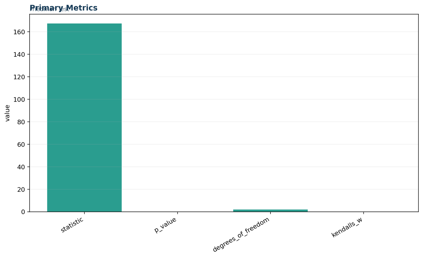
Python chart 1: Friedman test primary metrics
The primary metrics panel establishes the entire inferential result. It displays 649 complete student blocks, a tie-corrected Friedman Q of 167.3283, 2 degrees of freedom, a p-value far below .001, and Kendall’s W = 0.1289. The chart therefore separates statistical evidence from effect magnitude: the repeated grade difference is highly reliable, while the standardized effect remains modest.
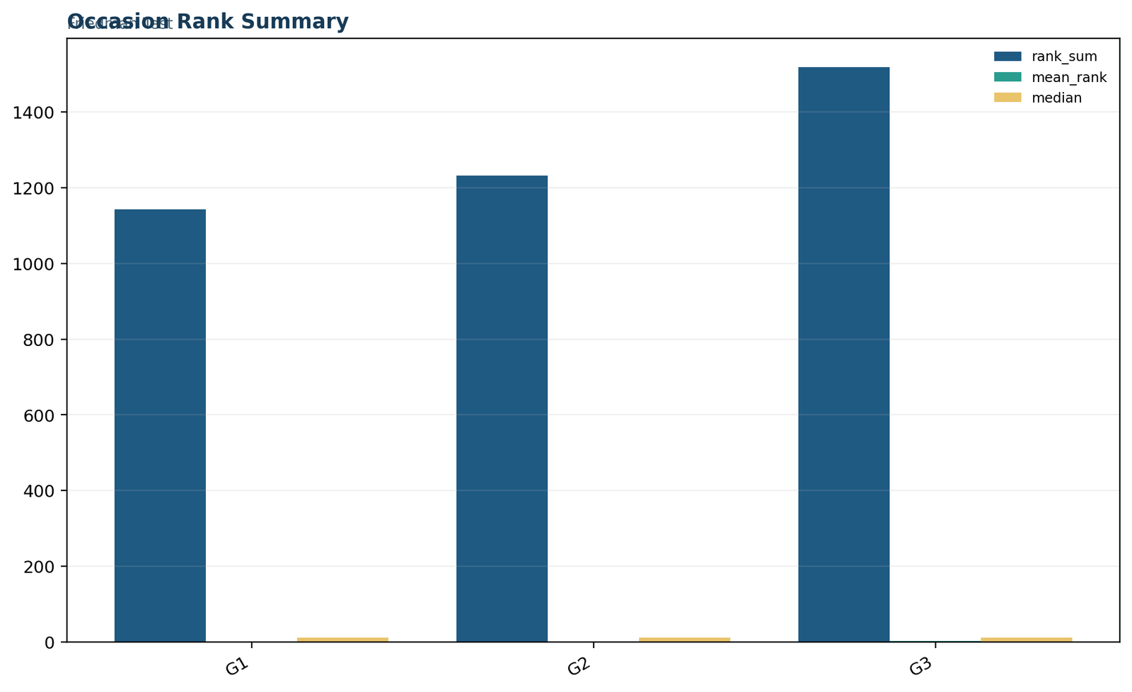
Python chart 2: occasion rank summary
The mean-rank ordering is the central descriptive result of the Friedman test. G1 has a mean rank of 1.7612, G2 has 1.8983, and G3 has 2.3405. Their corresponding rank sums are 1,143, 1,232, and 1,519. The visibly higher G3 rank shows that final grades tend to occupy the highest within-student position.
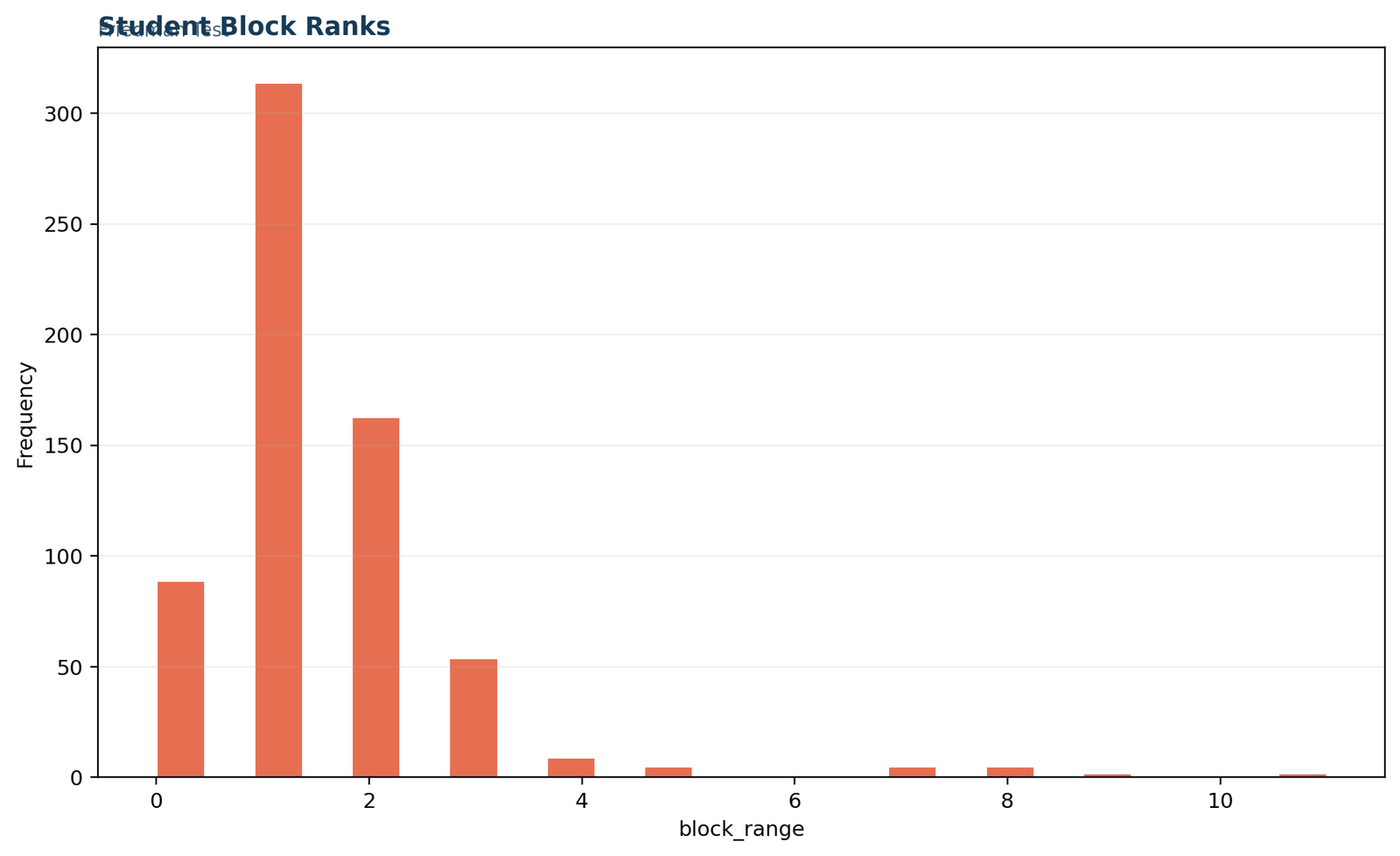
Python chart 3: student block ranks
This chart illustrates the defining operation of the Friedman test: every student’s G1, G2, and G3 values are ranked only against one another. A row such as 0, 11, 11 receives ranks 1, 2.5, 2.5, while a row such as 14, 14, 14 receives 2, 2, 2. The figure makes the block structure and average-rank treatment of ties visible rather than leaving them hidden inside a single chi-square statistic.
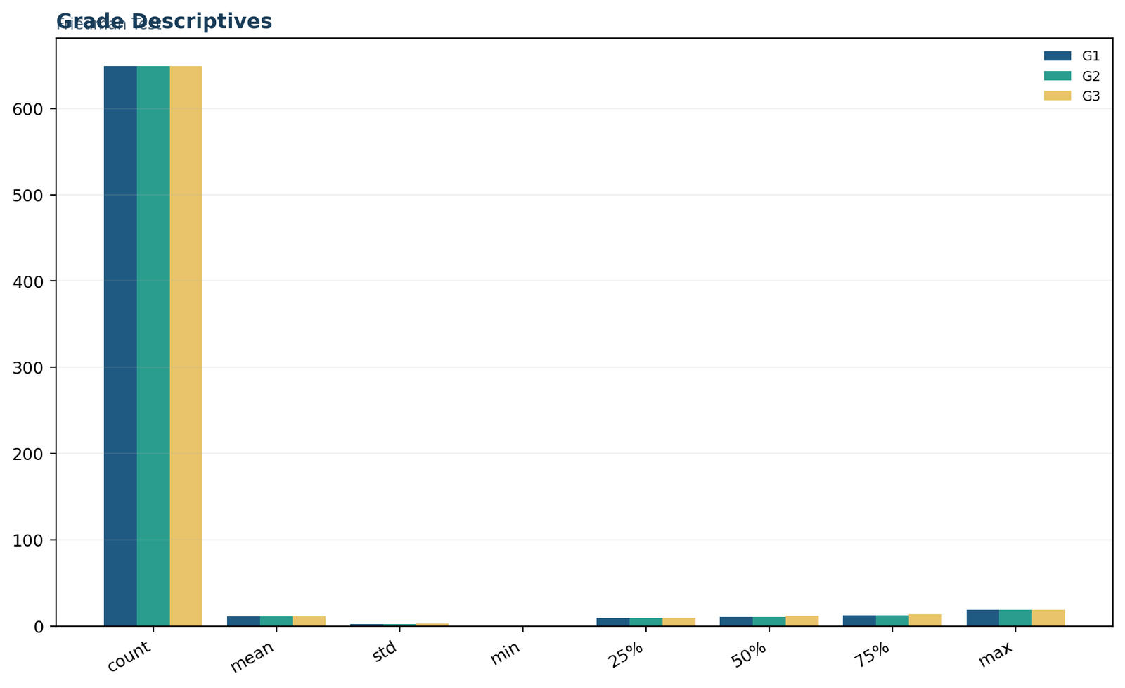
Python chart 4: grade descriptives
The raw descriptive pattern supports the rank-based result. Mean grades rise from 11.3991 for G1 to 11.5701 for G2 and 11.9060 for G3. Medians are 11, 11, and 12, while standard deviations are 2.7453, 2.9136, and 3.2307. These summaries explain the direction, but the Friedman test derives significance from repeated within-student ranks.
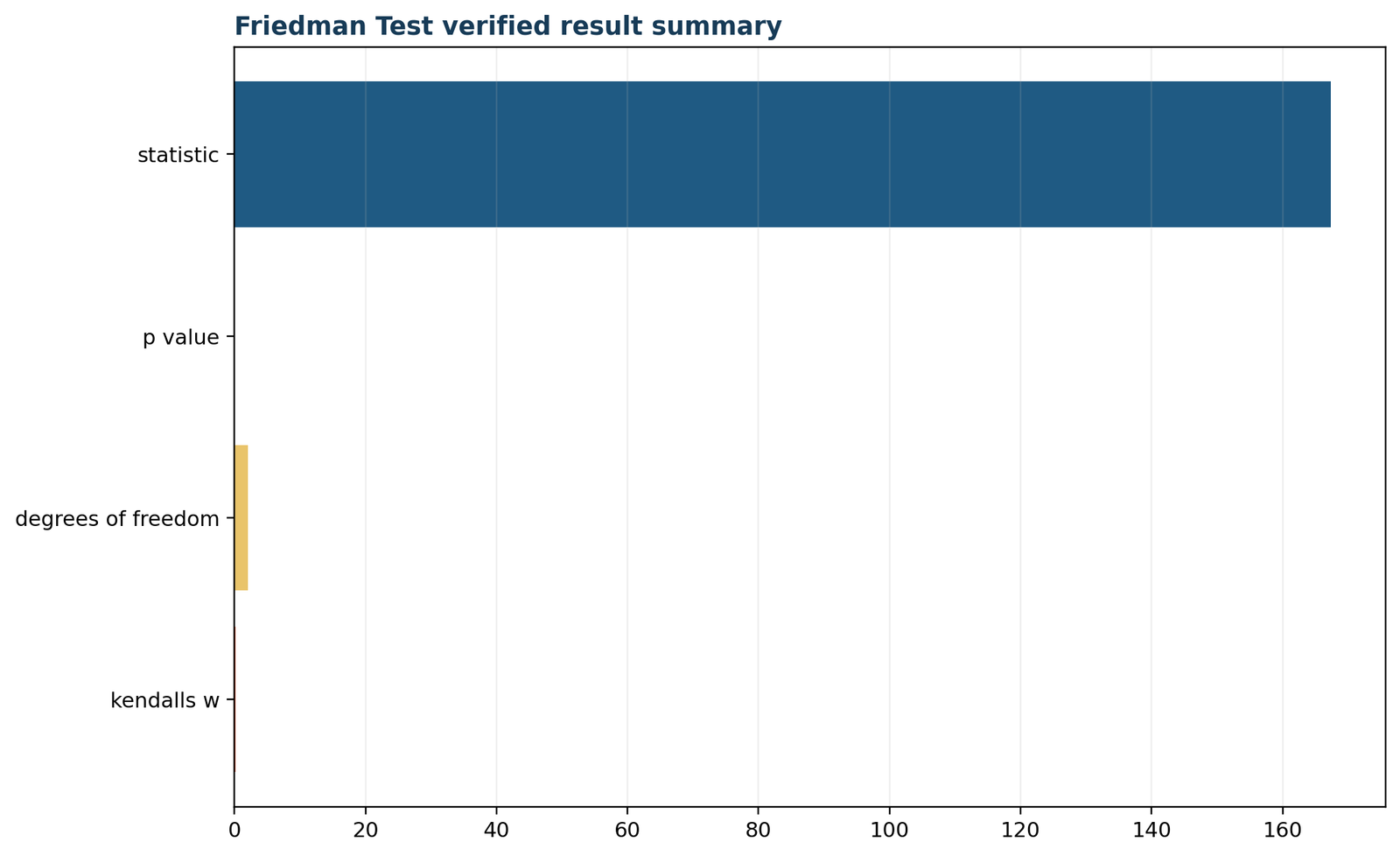
Python chart 5: verified result summary
The final Python chart consolidates the conclusion: the three grade occasions do not share the same rank distribution, G3 has the highest mean rank, and the omnibus effect is statistically significant with a modest Kendall’s W. It provides a compact visual equivalent of the full reporting paragraph without replacing the detailed numerical interpretation.
Friedman test in R: results and chart interpretation
R’s base implementation treats the data as an unreplicated complete-block design.
The keywords Friedman test in R, Friedman test R, and R Friedman test refer to the same workflow: arrange G1, G2, and G3 as related columns or reshape the data into response, group, and block variables. Related R resources include categorical data analysis in R, ANOVA in R, and correlation in R.
grades <- as.matrix(data[c("G1", "G2", "G3")])

result <- friedman.test(grades)

print(result)Q <- unname(result$statistic)

n <- nrow(grades)

k <- ncol(grades)

W <- Q / (n * (k - 1))

W
R chart 1: primary metrics
The R summary reproduces the same primary quantities as Python and Excel: Q = 167.3283, df = 2, p < .001, and W = 0.1289. Agreement across platforms confirms that the conclusion follows from the data and the tie-corrected Friedman formula rather than a software-specific default.
R chart 2: occasion rank summary
The R chart emphasizes the same monotonic rank pattern: G1 is lowest, G2 is slightly higher, and G3 is clearly highest. The gap between G2 and G3 is much larger than the gap between G1 and G2, which anticipates the strength of the paired post hoc comparisons.
R chart 3: block-level ranking
The block-rank display demonstrates why the Friedman test is a related-samples method. Every student’s three grades produce one local ranking. Averaging across these 649 local rank sets removes stable student-level differences and isolates the occasion effect.
R chart 4: descriptive grade profile
The descriptive profile shows an upward shift toward G3 along with slightly greater variability. The median increase from 11 to 12 is easy to communicate, while the rank analysis shows that the improvement pattern is not limited to a few extreme students.
R chart 5: verified conclusion
The final R figure brings the method, effect size, and decision together. The null of equal repeated-grade distributions is rejected, G3 is the highest-ranked occasion, and Kendall’s W describes the effect as modest rather than overwhelming.
How to do a Friedman test in SPSS
SPSS treats G1, G2, and G3 as several related samples.
Common searches include how to do a Friedman test in SPSS, how to run Friedman test in SPSS, and how to interpret Friedman test results. In wide-format data, each repeated occasion appears in a separate variable column and each row represents one subject.
SPSS menu structure
The related-samples nonparametric procedure compares G1, G2, and G3 inside each row. The output normally provides the number of cases, mean rank for each variable, the Friedman chi-square statistic, degrees of freedom, and asymptotic significance.
The same principles used in ANOVA in SPSS and categorical data analysis in SPSS apply to data preparation: variable labels, missing-value definitions, and row alignment must match the design.
SPSS syntax
NPAR TESTS

/FRIEDMAN = G1 G2 G3

/MISSING ANALYSIS.
The expected output is approximately χ²(2) = 167.328, p < .001, with mean ranks of 1.76, 1.90, and 2.34.
How to do the Friedman test in Excel
The workbook exposes every rank, tie term, intermediate quantity, and reporting value.
The query how to do Friedman test in Excel reflects the value of an auditable calculation. Excel does not need to hide the method behind a single function: each student row can be ranked, condition rank sums can be added, the tie correction can be calculated, and the chi-square p-value can be obtained from the corrected Q statistic.
| Workbook sheet | Role in the Friedman test analysis | Key content |
|---|---|---|
| Guide | Defines design and variables | Three repeated grades with students as complete blocks. |
| Data_Input | Stores unchanged raw values | G1, G2, and G3 for 649 students. |
| Working | Shows row-level lineage | Within-student ranks, range ranks, weighted scores, and tie terms. |
| Calculations | Builds omnibus statistics | Rank sums, mean ranks, Friedman Q, Kendall’s W, Page and Quade sensitivity quantities. |
| Diagnostics | Documents design checks | Blocking, tie handling, and method identity. |
| Reporting | Cross-checks verified results | Q = 167.328277 and W = 0.128912 with zero calculation difference. |
Row rank formulas
Each G1:G3 row is ranked in ascending order. Average ranks are required for ties. Column sums of the three rank columns produce RG1, RG2, and RG3.
Excel workflows can be reviewed alongside regression in Excel, correlation in Excel, and t-test in Excel.
P-value formula
After computing the tie-corrected Q, the right-tail chi-square probability is obtained with 2 degrees of freedom. The workbook result rounds to zero at ordinary display precision, while the more precise probability is approximately 4.63 × 10−37.
Displaying p < .001 is clearer than reporting p = 0, because a continuous reference probability is extremely small rather than literally zero.
Post hoc comparisons after a significant Friedman test
The omnibus result establishes a difference but does not identify every pair.
After rejecting the Friedman test null hypothesis, related-samples pairwise comparisons can be performed with Wilcoxon signed-rank tests and a multiplicity adjustment such as Holm. The same subjects must remain paired in every comparison.
| Pair | Wilcoxon statistic | Raw p-value | Holm-adjusted p-value | Direction |
|---|---|---|---|---|
| G1 vs G2 | 43,328.0 | 0.0003473 | 0.0003473 | G2 is generally higher than G1. |
| G1 vs G3 | 25,595.5 | 5.57 × 10⁻²⁴ | 1.11 × 10⁻²³ | G3 is generally higher than G1. |
| G2 vs G3 | 13,701.0 | 7.26 × 10⁻²⁵ | 2.18 × 10⁻²⁴ | G3 is generally higher than G2. |
G1 to G2
Among 649 students, 273 had G2 above G1, 187 had G2 below G1, and 189 were tied. The pairwise shift is smaller than the changes involving G3 but remains significant after Holm adjustment.
G1 to G3
G3 exceeded G1 for 344 students, was lower for 120, and tied for 185. The median paired difference was 1 grade point, and the adjusted p-value was far below .001.
G2 to G3
G3 exceeded G2 for 290 students, was lower for 72, and tied for 287. Despite many ties, the positive direction was highly systematic.
Friedman test vs repeated-measures ANOVA and related methods
Method choice follows the dependence structure, outcome scale, and research question.
The difference between Kruskal Wallis and Friedman test is especially important: Kruskal–Wallis compares independent groups, whereas the Friedman test compares related conditions or treatments within blocks.
| Method | Design | Outcome / model focus | Relationship to Friedman test |
|---|---|---|---|
| Friedman test | Three or more related conditions | Within-block ranks | Primary method in this article. |
| Repeated-measures ANOVA | Three or more related conditions | Parametric mean model | Uses normal-theory assumptions and may require sphericity corrections. |
| Kruskal–Wallis test | Three or more independent groups | Independent-group ranks | Not appropriate for repeated observations on the same students. |
| Wilcoxon signed-rank test | Two related conditions | Paired rank differences | Useful for post hoc pairs after Friedman. |
| Sign test | Two related conditions | Direction of paired differences | More minimal assumptions but often less powerful. |
| Cochran’s Q | Three or more related binary conditions | Repeated binary outcomes | Binary-data analogue of a repeated omnibus test. |
| Quade test | Complete blocks | Weighted within-block ranks | Can gain sensitivity when block ranges contain useful information. |
| Page test | Related ordered conditions | Prespecified monotonic trend | Targets an ordered alternative rather than any difference. |
Quade sensitivity result
The workbook’s Quade calculation produced F = 91.1481 with p far below .001. It weights block rank differences by the range of scores within each student, giving more influence to blocks that show larger separation across occasions.
Page trend result
With the prespecified order G1 → G2 → G3, the workbook produced Page L = 8,164 and z = 10.4364, again indicating a strong upward ordered trend. The Page test addresses a narrower directional question than the omnibus Friedman test.
Researchers comparing model families may also review mixed ANOVA, multilevel regression, and ordinal logistic regression.
Friedman test diagnostics and design checks
Quality control focuses on block completeness, ties, ordering, and the meaning of the repeated occasions.
The Friedman test does not use residual normality diagnostics, but careful analysis still checks the data structure and the interpretability of the rank comparison.
Complete-block verification
Missing repeated measurements can change the usable sample and may motivate a model-based longitudinal method. General missing-data structure is different from the outlier and influence issues covered under outlier detection and influence diagnostics.
Tie and shape assessment
The descriptive distributions differ slightly in spread, especially for G3. The safest omnibus wording is therefore a difference in repeated grade distributions or rank positions, followed by the explicit descriptive direction.
Complete blocks, missing occasions, and analysis population
The classical complete-block calculation uses only subjects with one valid response at every repeated occasion. That requirement makes the analysis population explicit: the 649 students in this example are the students for whom G1, G2, and G3 can all be ranked within the same row. If an occasion is missing, there is no complete three-way ordering for that block, so the ordinary rank-sum formula cannot use the row unchanged.
Complete-case analysis is easy to audit, but its interpretation depends on why records are incomplete. When missingness is related to performance, attendance, treatment response, or another measured process, the complete blocks may differ systematically from the original cohort. Longitudinal modeling with mixed-effects regression, generalized estimating equations, or a suitable multilevel regression can retain partially observed subjects under stated modeling assumptions.
For the present grade analysis, the block count is stable across the workbook, Python, R, and SPSS outputs. That consistency is important because a changed case count would alter the rank sums, tie correction, degrees of freedom calculation, effect-size denominator, and every post hoc comparison.
Asymptotic inference, exact inference, and large samples
The chi-square reference distribution is an asymptotic approximation. It becomes accurate as the number of independent blocks grows, provided the design is valid and no small collection of unusual blocks dominates the ranking pattern. With 649 complete student blocks, the approximation is well supported, and the resulting probability is so small that minor reference-distribution differences would not change the decision.
Small studies can use exact or permutation-based reasoning when software supports it. Exact inference enumerates or otherwise evaluates the possible within-block rank arrangements under the null. Permutation methods repeatedly rearrange condition labels within blocks, preserving the dependence structure while measuring how unusual the observed rank sums are. Both approaches respect the essential blocking principle; labels are never shuffled freely between different students.
The distinction mirrors the broader difference between approximate and exact procedures discussed in Fisher’s exact test, Barnard’s exact test, and the binomial test. In every case, the reference method should match the sample structure and be stated in the report.
Interpreting an ordered pattern without overstating growth
The descriptive means and mean ranks increase from G1 through G3, and the Page trend calculation supports the prespecified order G1 < G2 < G3. Even so, the repeated grade pattern is not identical for all students. G2 is below G1 for 187 students, and G3 is below G1 for 120 students. The omnibus result therefore describes a population-level tendency rather than a universal individual trajectory.
This distinction is important in educational, medical, and behavioral repeated-measures research. A statistically significant average rank progression can coexist with stable cases, reversals, and heterogeneous response profiles. The effect-size value W = 0.1289 captures some of that heterogeneity: the occasions differ reliably, but the within-block ordering is far from perfectly concordant.
When individual trajectories are scientifically important, line plots, transition summaries, and subject-specific models add information beyond the omnibus rank result. The current student-block chart provides a visual starting point, while methods such as hierarchical linear models and random-effects regression can represent variation in starting level and change across students.
How to report Friedman test results in APA style
A complete report includes the design, descriptives, statistic, effect size, and adjusted follow-up findings.
Searches for how to report Friedman test results and how to report Friedman test results APA call for a concise paragraph that remains statistically complete.
APA-style example
A Friedman test showed that grades differed significantly across G1, G2, and G3, χ2F(2, N = 649) = 167.33, p < .001, Kendall’s W = .129. Mean ranks increased from G1 (Mrank = 1.76) to G2 (Mrank = 1.90) and G3 (Mrank = 2.34). Holm-adjusted Wilcoxon signed-rank comparisons indicated significant differences between G1 and G2 (p = .00035), G1 and G3 (p < .001), and G2 and G3 (p < .001). Descriptively, mean grades were 11.40, 11.57, and 11.91, respectively.
Minimum reporting elements
- Name the Friedman test and repeated conditions.
- State the number of complete blocks.
- Report Q or χ²F, df, and p.
- Report mean ranks for direction.
- Include Kendall’s W.
- Name the post hoc test and p-value adjustment.
Interpretation language
- Use “differed significantly across occasions” for the omnibus result.
- Use mean ranks and descriptives to explain direction.
- Use “p < .001” rather than p = 0.
- Describe W as a magnitude indicator, not another hypothesis test.
- Keep association language separate from causal claims unless the design supports causality.
Additional reporting foundations appear in confidence intervals, margin of error, and statistical power.
Friedman test downloads and related guides
Reports, workbook, and contextual statistical resources.
Python reportthe procedure metrics, ranks, charts, and verified interpretation.Open Python PDF
R reportRepeated-samples rank analysis and matching result summary.Open R PDF
SPSS outputSeveral-related-samples output for G1, G2, and G3.Open SPSS PDF
Excel workbookAuditable ranks, tie correction, effect size, and reporting sheets.Open Excel workbook
Related statistical guides
Frequently asked questions about the the procedure
Direct answers to the main the procedure search questions.
What is a the procedure?
The the procedure is a nonparametric omnibus procedure for comparing three or more related conditions. It ranks the condition values within each subject or block and tests whether the condition rank sums differ more than expected under the null hypothesis.
What is the the procedure used for?
It is used for repeated-measures or complete-block designs when the outcome is ordinal or continuous and a rank-based alternative to repeated-measures ANOVA is appropriate.
When should the the procedure be used?
Use the the procedure when the same subjects are observed under at least three conditions, every block contains each condition, and the research question concerns an omnibus difference across those related measurements.
Does the the procedure require normality?
No. The method uses within-block ranks and does not require normally distributed residuals. It still requires a valid related-samples structure and meaningful ranking.
What are the assumptions of the the procedure?
The observations must be related within blocks and independent between blocks; the outcome must be rankable; the same conditions must be measured for each complete block; and the condition labels must represent comparable repeated treatments or occasions.
What is the difference between Kruskal–Wallis and the procedure?
Kruskal–Wallis compares independent groups. The the procedure compares related conditions measured on the same subjects or matched blocks.
Is the the procedure a nonparametric ANOVA?
It is commonly described as the nonparametric alternative to one-way repeated-measures ANOVA. The description is useful, although the the procedure evaluates ranks rather than fitting the same mean-based model.
What is the null hypothesis of the the procedure?
The null states that the related conditions have the same distributional location or no systematic difference in rank position across blocks.
How is the Friedman statistic calculated?
Values are ranked within each block, ranks are summed by condition, and the squared condition rank sums are inserted into the Friedman formula. A correction is applied when ties occur.
What does a significant the procedure mean?
It means at least one related condition differs from the others. Post hoc paired comparisons are needed to determine the specific pairs.
How is the the procedure interpreted here?
G1, G2, and G3 differed significantly, Q(2) = 167.33, p < .001. G3 had the highest mean rank, and all three paired comparisons remained significant after Holm adjustment.
What is Kendall’s W in the the procedure?
Kendall’s W is a standardized effect-size or concordance measure. Here W = 0.1289, indicating a modest repeated-occasion effect.
How do ties affect the the procedure?
Tied values receive average ranks. A tie correction adjusts the statistic because ties reduce the variability of possible rank arrangements.
How do I run a the procedure in R?
Place the repeated conditions in aligned columns and use friedman.test() on the matrix, or supply response, group, and block variables in long format.
How do I run a the procedure in Python?
Use SciPy’s friedmanchisquare() with one aligned array per repeated condition.
How do I run a the procedure in SPSS?
Use the several-related-samples nonparametric procedure with G1, G2, and G3 as the related variables, or use the NPAR TESTS /FRIEDMAN syntax.
How can the the procedure be calculated in Excel?
Rank each row across the repeated conditions, sum the ranks by column, calculate Q, apply the within-row tie correction, and obtain the upper-tail chi-square probability with k − 1 degrees of freedom.
Which post hoc test follows the the procedure?
Pairwise Wilcoxon signed-rank tests with Holm adjustment are a common follow-up. Other specialized repeated-rank multiple-comparison procedures are also available.