
.pcs-wrap{–ink:#172033;–muted:#607083;–navy:#123b5d;–blue:#176ea6;–teal:#087f6b;–amber:#b86b10;–rose:#a33a54;–line:#d8e3ea;–soft:#f5f9fc;–soft2:#eefbf8;–warn:#fff7e8;–danger:#fff1f2;–code:#101828;max-width:1120px;margin:0 auto;color:var(–ink);font-family:system-ui,-apple-system,BlinkMacSystemFont,”Segoe UI”,Arial,sans-serif;line-height:1.76}
.pcs-wrap *{box-sizing:border-box}.pcs-wrap h1,.pcs-wrap h2,.pcs-wrap h3,.pcs-wrap h4{line-height:1.25}.pcs-wrap h2{font-size:30px;color:var(–navy);margin:0 0 16px}.pcs-wrap h3{font-size:23px;color:#245877;margin:28px 0 12px}.pcs-wrap h4{font-size:18px;color:#263c52;margin:22px 0 9px}.pcs-wrap p{margin:0 0 16px}.pcs-wrap a{color:#0b6598;text-decoration:underline}.pcs-wrap li{margin:7px 0}
.pcs-hero{padding:36px;border:1px solid var(–line);border-radius:26px;background:linear-gradient(135deg,#eef7fb 0%,#fff 52%,#fff4e7 100%);box-shadow:0 14px 36px rgba(24,59,86,.08);margin:14px 0 26px}
.pcs-kicker{display:inline-flex;align-items:center;gap:8px;padding:7px 13px;border-radius:999px;background:#e7f6f3;border:1px solid #bce5dc;color:#075f52;font-size:13px;font-weight:800;letter-spacing:.04em;text-transform:uppercase;margin-bottom:15px}
.pcs-hero h1{font-size:43px;color:#102e46;margin:0 0 16px}.pcs-hero p{font-size:20px;color:#2b3b4e;margin:0}.pcs-badges{display:flex;flex-wrap:wrap;gap:10px;margin-top:22px}.pcs-badge{padding:8px 12px;border-radius:999px;border:1px solid var(–line);background:#fff;font-weight:750;font-size:14px}
.pcs-ad{padding:18px;border:1px dashed #aebbc8;border-radius:16px;text-align:center;color:#718096;background:#fcfdfe;margin:27px 0}.pcs-ad span{display:block;font-size:11px;text-transform:uppercase;letter-spacing:.1em;margin-bottom:4px}
.pcs-section{background:#fff;border:1px solid var(–line);border-radius:22px;padding:25px;margin:24px 0;box-shadow:0 8px 24px rgba(15,23,42,.035)}
.pcs-note{background:#f5f9fd;border-left:5px solid var(–navy);border-radius:16px;padding:18px 20px;margin:19px 0}.pcs-success{background:#ecfdf5;border:1px solid #bbf7d0;border-radius:17px;padding:18px 20px;margin:19px 0}.pcs-warning{background:var(–warn);border:1px solid #f1d19b;border-radius:17px;padding:18px 20px;margin:19px 0}.pcs-danger{background:var(–danger);border:1px solid #fecdd3;border-radius:17px;padding:18px 20px;margin:19px 0}
.pcs-stat-grid{display:grid;grid-template-columns:repeat(4,minmax(0,1fr));gap:14px;margin:20px 0}.pcs-stat{padding:17px;border:1px solid var(–line);border-radius:17px;background:var(–soft)}.pcs-stat small{display:block;color:var(–muted);margin-bottom:6px}.pcs-stat strong{display:block;font-size:23px;color:var(–navy)}
.pcs-result-grid{display:grid;grid-template-columns:1fr 1fr;gap:18px;margin:20px 0}.pcs-result{border:1px solid var(–line);border-radius:19px;padding:20px}.pcs-result.method{background:#f1f8fc}.pcs-result.meaning{background:#f0fbf7}.pcs-result h3{margin:0 0 8px}.pcs-result ul{margin:10px 0 0;padding-left:20px}
.pcs-toc{columns:2;column-gap:34px;margin:0;padding-left:20px}.pcs-toc li{break-inside:avoid;margin:8px 0}
.pcs-problem-grid{display:grid;grid-template-columns:repeat(3,minmax(0,1fr));gap:15px}.pcs-problem{border:1px solid var(–line);border-radius:18px;padding:18px;background:var(–soft)}.pcs-problem strong{display:block;font-size:20px;color:var(–navy);margin-bottom:5px}.pcs-problem span{color:var(–muted)}
.pcs-flow{display:grid;grid-template-columns:1fr auto 1fr auto 1fr;gap:12px;align-items:stretch;margin:22px 0}.pcs-step{border:1px solid var(–line);border-radius:18px;padding:19px;background:#fff}.pcs-step b{display:block;color:var(–teal);font-size:13px;text-transform:uppercase;letter-spacing:.05em;margin-bottom:7px}.pcs-arrow{display:flex;align-items:center;font-size:28px;color:#8aa0b2;font-weight:800}
.pcs-formula{padding:18px;border:1px solid var(–line);border-radius:17px;text-align:center;background:#f7f9fc;font-weight:800;font-size:19px;color:var(–navy);margin:18px 0;overflow-x:auto}
.pcs-table-wrap{overflow-x:auto;border:1px solid var(–line);border-radius:18px;margin:18px 0}.pcs-table{width:100%;min-width:880px;border-collapse:collapse;background:#fff}.pcs-table th{background:#edf5f9;color:#163d58;text-align:left;padding:12px;border-bottom:1px solid var(–line)}.pcs-table td{padding:12px;border-bottom:1px solid #edf1f4;vertical-align:top}.pcs-table tr:last-child td{border-bottom:none}
.pcs-decision-grid{display:grid;grid-template-columns:repeat(2,minmax(0,1fr));gap:16px;margin:20px 0}.pcs-decision{border:1px solid var(–line);border-radius:18px;padding:19px;background:#fff}.pcs-decision h3{margin-top:0}.pcs-decision.use{border-top:5px solid var(–teal)}.pcs-decision.avoid{border-top:5px solid var(–amber)}
.pcs-method-grid{display:grid;grid-template-columns:repeat(4,minmax(0,1fr));gap:13px;margin:20px 0}.pcs-method{border:1px solid var(–line);border-radius:17px;padding:17px;background:#fff}.pcs-method strong{display:block;color:var(–navy);font-size:18px;margin-bottom:7px}.pcs-method p{font-size:14px;color:#405368;margin:0}
.pcs-chart-story{border-top:1px solid var(–line);padding:30px 0 8px}.pcs-chart-story:first-of-type{border-top:none;padding-top:4px}.pcs-figure{margin:16px 0 18px;border:1px solid var(–line);border-radius:20px;overflow:hidden;background:#fff}.pcs-figure img{display:block;width:100%;height:auto}.pcs-figure figcaption{padding:13px 16px;background:#fbfdff;border-top:1px solid var(–line);color:var(–muted);font-size:14px}
.pcs-insight-grid{display:grid;grid-template-columns:1fr 1fr;gap:13px}.pcs-insight{border:1px solid var(–line);border-radius:16px;padding:16px;background:#fff}.pcs-insight span{display:block;font-size:12px;font-weight:850;letter-spacing:.06em;text-transform:uppercase;color:var(–teal);margin-bottom:7px}.pcs-insight p{margin:0}.pcs-next{margin:13px 0 0;padding:13px 15px;border-radius:14px;background:#f3f7fb;color:#405368;font-size:14px}
.pcs-metric-grid{display:grid;grid-template-columns:repeat(3,minmax(0,1fr));gap:14px}.pcs-metric{border:1px solid var(–line);border-radius:17px;padding:17px;background:#fff}.pcs-metric b{display:block;color:var(–navy);margin-bottom:6px}.pcs-metric strong{font-size:20px;color:var(–teal)}
.pcs-software-grid{display:grid;grid-template-columns:repeat(2,minmax(0,1fr));gap:16px}.pcs-software{border:1px solid var(–line);border-radius:18px;padding:19px}.pcs-software h3{margin:0 0 8px}.pcs-software ul{padding-left:19px;margin:8px 0}
.pcs-details details{border:1px solid var(–line);border-radius:15px;padding:14px 16px;margin:11px 0;background:#fff}.pcs-details summary{cursor:pointer;font-weight:850;color:var(–navy)}.pcs-details details>div{padding-top:13px}
.pcs-code{background:var(–code);color:#e5e7eb;border-radius:17px;padding:17px;overflow-x:auto;font-size:13.5px;line-height:1.62}.pcs-code code{font-family:Consolas,Monaco,”Courier New”,monospace}
.pcs-two-col{display:grid;grid-template-columns:1fr 1fr;gap:18px}.pcs-list-card{border:1px solid var(–line);border-radius:18px;padding:19px;background:#fff}.pcs-list-card h3{margin:0 0 9px}.pcs-list-card ul{padding-left:20px;margin:0}
.pcs-apa-grid{display:grid;grid-template-columns:1fr 1fr;gap:16px;margin:18px 0}.pcs-report{border:1px solid var(–line);border-radius:18px;padding:19px;background:#fff}.pcs-report h3{margin:0 0 10px}.pcs-copy{border-left:5px solid var(–teal);background:#f0fbf7;border-radius:15px;padding:17px 19px;margin:14px 0}.pcs-copy p:last-child{margin-bottom:0}.pcs-template{border:1px dashed #9fb0bf;border-radius:15px;background:#fbfdff;padding:16px;margin:12px 0}.pcs-template code{white-space:normal;color:#20364a;font-family:inherit}
.pcs-r-pair{margin:28px 0 34px;padding:20px;border:1px solid var(–line);border-radius:21px;background:#fbfdff}.pcs-r-pair-title{margin:0 0 15px;font-size:17px;color:var(–navy);font-weight:850}.pcs-r-chart-row{display:grid;grid-template-columns:repeat(2,minmax(0,1fr));gap:18px;align-items:start}.pcs-r-chart-box{border:1px solid var(–line);border-radius:18px;overflow:hidden;background:#fff}.pcs-r-chart-box figure{margin:0}.pcs-r-chart-box img{display:block;width:100%;height:auto}.pcs-r-chart-box figcaption{padding:12px 14px;background:#f7fafc;border-top:1px solid var(–line);color:var(–muted);font-size:13px}.pcs-r-explanation-row{display:grid;grid-template-columns:repeat(2,minmax(0,1fr));gap:18px;margin-top:14px}.pcs-r-explanation{border:1px solid var(–line);border-radius:17px;padding:17px;background:#fff}.pcs-r-explanation h3{font-size:19px;margin:0 0 9px}.pcs-r-label{display:block;font-size:12px;font-weight:850;letter-spacing:.06em;text-transform:uppercase;color:var(–teal);margin-bottom:6px}.pcs-r-check{padding:11px 13px;border-radius:13px;background:#eef7fb;color:#405368;font-size:13px;margin-top:10px}
.pcs-download-grid{display:grid;grid-template-columns:repeat(2,minmax(0,1fr));gap:14px}.pcs-download{display:block;text-decoration:none!important;border:1px solid var(–line);border-radius:17px;padding:18px;background:#fff}.pcs-download strong{display:block;color:var(–navy);font-size:18px;margin-bottom:5px}.pcs-download span{color:var(–muted);font-size:14px}.pcs-related{display:grid;grid-template-columns:repeat(2,minmax(0,1fr));gap:11px}.pcs-related a{display:block;padding:12px 14px;border:1px solid var(–line);border-radius:14px;background:#f8fafc;text-decoration:none}.pcs-faq details{border:1px solid var(–line);border-radius:15px;padding:15px 17px;margin:10px 0}.pcs-faq summary{cursor:pointer;font-weight:850;color:var(–navy)}.pcs-faq p{margin-top:11px}
html{scroll-behavior:smooth}.pcs-top-anchor{position:absolute;top:0;left:0;width:1px;height:1px;overflow:hidden}.pcs-back-to-top{position:fixed;right:22px;bottom:24px;width:48px;height:48px;display:flex;align-items:center;justify-content:center;border-radius:50%;background:var(–navy);color:#fff!important;text-decoration:none!important;font-size:25px;font-weight:900;box-shadow:0 10px 24px rgba(15,23,42,.24);z-index:9999;border:2px solid rgba(255,255,255,.85)}.pcs-back-to-top:hover{background:var(–teal);transform:translateY(-3px)}.pcs-back-to-top span{position:absolute;width:1px;height:1px;overflow:hidden;clip:rect(0,0,0,0)}
@media(max-width:900px){.pcs-method-grid{grid-template-columns:repeat(2,1fr)}.pcs-stat-grid,.pcs-metric-grid{grid-template-columns:repeat(2,1fr)}.pcs-result-grid,.pcs-two-col,.pcs-software-grid,.pcs-download-grid,.pcs-related,.pcs-insight-grid,.pcs-apa-grid,.pcs-decision-grid,.pcs-r-chart-row,.pcs-r-explanation-row{grid-template-columns:1fr}.pcs-flow{grid-template-columns:1fr}.pcs-arrow{justify-content:center;transform:rotate(90deg)}.pcs-toc{columns:1}.pcs-problem-grid{grid-template-columns:1fr}.pcs-hero h1{font-size:34px}}
@media(max-width:540px){.pcs-stat-grid,.pcs-metric-grid,.pcs-method-grid{grid-template-columns:1fr}.pcs-section,.pcs-hero{padding:21px}.pcs-hero h1{font-size:29px}.pcs-hero p{font-size:17px}.pcs-wrap h2{font-size:25px}.pcs-back-to-top{right:15px;bottom:18px;width:44px;height:44px}}
/* Readable APA templates: deliberately avoid theme styling. */
.pcs-template{
border:1px dashed #9fb0bf!important;
border-radius:15px!important;
background:#fbfdff!important;
padding:17px 19px!important;
margin:13px 0 20px!important;
color:#20364a!important;
box-shadow:none!important;
}
.pcs-template,
.pcs-template *{
color:#20364a!important;
background:transparent!important;
text-shadow:none!important;
box-shadow:none!important;
}
.pcs-template-text{
display:block!important;
margin:0!important;
padding:0!important;
border:0!important;
font-family:system-ui,-apple-system,BlinkMacSystemFont,"Segoe UI",Arial,sans-serif!important;
font-size:16px!important;
font-weight:400!important;
line-height:1.78!important;
white-space:normal!important;
word-break:normal!important;
overflow-wrap:anywhere!important;
}
/* Final APA reporting cards */
.pcs-apa-template-intro{
display:flex;
align-items:flex-start;
gap:12px;
padding:15px 17px;
margin:16px 0 18px;
border:1px solid #c9d9e5;
border-radius:15px;
background:#f5faff;
color:#29435a
}
.pcs-apa-template-intro strong{color:var(--navy)}
.pcs-apa-template-grid{
display:grid;
grid-template-columns:repeat(2,minmax(0,1fr));
gap:16px;
margin:16px 0 24px
}
.pcs-apa-template-card{
border:1px solid var(--line);
border-radius:19px;
padding:19px;
background:#fff;
box-shadow:0 5px 16px rgba(15,23,42,.035)
}
.pcs-apa-template-card.directional{grid-column:1/-1}
.pcs-apa-template-head{
display:flex;
flex-wrap:wrap;
align-items:center;
gap:10px;
margin-bottom:13px
}
.pcs-apa-template-head h4{
margin:0;
color:var(--navy);
font-size:20px
}
.pcs-apa-status{
display:inline-flex;
align-items:center;
border-radius:999px;
padding:5px 10px;
font-size:12px;
line-height:1.2;
font-weight:850;
letter-spacing:.035em;
text-transform:uppercase
}
.pcs-apa-status.ns{background:#eef4f8;color:#39556b;border:1px solid #cbd8e1}
.pcs-apa-status.sig{background:#ecfdf5;color:#076451;border:1px solid #b7e8da}
.pcs-apa-status.one{background:#fff7e8;color:#8a520a;border:1px solid #efcf98}
.pcs-apa-template-copy{
border-left:5px solid var(--blue);
border-radius:14px;
background:#f8fbfe;
padding:16px 17px;
color:#20364a
}
.pcs-apa-template-card.sig-card .pcs-apa-template-copy{border-left-color:var(--teal)}
.pcs-apa-template-card.directional .pcs-apa-template-copy{border-left-color:var(--amber)}
.pcs-apa-template-copy p{
margin:0 0 11px!important;
color:#20364a!important;
font-size:16px!important;
line-height:1.72!important
}
.pcs-apa-template-copy p:last-child{margin-bottom:0!important}
.pcs-slot{
display:inline-block;
border:1px solid #b9d2e3;
border-radius:7px;
background:#eaf5fc;
color:#164e72;
padding:1px 6px;
margin:1px 1px;
font-weight:750;
white-space:nowrap
}
.pcs-apa-template-card.sig-card .pcs-slot{
border-color:#b6dfd4;
background:#eaf9f5;
color:#086653
}
.pcs-apa-template-card.directional .pcs-slot{
border-color:#e3c68d;
background:#fff5df;
color:#87510b
}
.pcs-template-tip{
display:block;
margin-top:11px;
color:var(--muted);
font-size:13px
}
/* One presentation for charts shared by Python and R */
.pcs-cross-software{
padding:16px 18px;
border:1px solid #c8dfd8;
border-radius:16px;
background:#f0fbf7;
margin:16px 0 22px;
color:#284b43
}
.pcs-chart-badge{
display:inline-flex;
margin-left:8px;
padding:4px 9px;
border-radius:999px;
border:1px solid #c8d8e3;
background:#f3f8fb;
color:#36566d;
font-size:11px;
font-weight:800;
letter-spacing:.035em;
text-transform:uppercase;
vertical-align:middle
}
@media(max-width:850px){
.pcs-apa-template-grid{grid-template-columns:1fr}
.pcs-apa-template-card.directional{grid-column:auto}
}
/* Final robust APA-template layout */
.pcs-apa-template-grid{display:block!important;margin:16px 0 24px!important}
.pcs-apa-template-card,.pcs-apa-template-card.directional{
display:block!important;width:100%!important;grid-column:auto!important;
margin:0 0 18px!important;padding:20px!important;overflow:visible!important
}
.pcs-apa-template-head{
display:flex!important;align-items:center!important;flex-wrap:wrap!important;
gap:10px!important;margin:0 0 13px!important
}
.pcs-apa-template-head h4{margin:0!important;font-size:21px!important;line-height:1.3!important}
.pcs-apa-template-copy{display:block!important;width:100%!important;padding:4px 17px!important}
.pcs-template-row{
display:grid!important;grid-template-columns:118px minmax(0,1fr)!important;
gap:14px!important;align-items:start!important;padding:13px 0!important;
border-bottom:1px solid #dce7ee!important
}
.pcs-template-row:last-child{border-bottom:0!important}
.pcs-template-label{
display:block!important;color:#31566f!important;font-size:12px!important;
line-height:1.35!important;font-weight:800!important;letter-spacing:.055em!important;
text-transform:uppercase!important;padding-top:4px!important
}
.pcs-template-row p{
display:block!important;margin:0!important;color:#20364a!important;
font-size:16px!important;line-height:1.75!important;min-width:0!important
}
.pcs-field{
display:inline!important;padding:1px 4px!important;border-radius:4px!important;
background:#eaf5fc!important;color:#145274!important;font-weight:750!important;
box-decoration-break:clone;-webkit-box-decoration-break:clone
}
.pcs-apa-template-card.sig-card .pcs-field{background:#eaf9f5!important;color:#086653!important}
.pcs-apa-template-card.directional .pcs-field{background:#fff3d9!important;color:#81500c!important}
.pcs-template-tip{
display:block!important;margin-top:12px!important;padding-top:11px!important;
border-top:1px dashed #cbd9e2!important;color:var(--muted)!important;font-size:13px!important
}
@media(max-width:650px){
.pcs-template-row{grid-template-columns:1fr!important;gap:5px!important}
.pcs-template-label{padding-top:0!important}
}
Pearson Chi-Square Test: Formula, Interpretation, Calculator, Python, R, SPSS and Excel Guide
The Pearson Chi-Square Test evaluates whether two categorical variables are statistically independent by comparing observed counts with the counts expected under the null hypothesis. This complete guide develops the formula cell by cell, verifies the assumptions, interprets residuals and contributions, compares Pearson with likelihood-ratio and exact procedures, and reproduces a worked 2 × 4 analysis in Python, R, SPSS, Stata and Excel.
2 × 4 contingency table
χ²(3) = 8.8857
p = 0.03085
Cramér’s V = 0.1170
Pearson Chi-Square Test Model Overview
The Pearson Chi-Square Test, also called the Pearson chi-squared test or Pearson’s chi-square test, evaluates whether observed categorical counts differ from the counts expected under a null model. In an independence analysis, it asks whether two categorical variables are statistically associated.
What Question Does It Answer?
The worked analysis asks whether a recorded two-level F/M group and a four-level G3 final-grade band are independent. The grade bands are low (G3 < 10), medium (10–13), high (14–16) and very high (17+).
How the Pearson Chi-Square Test Is Built
The method calculates the expected count for every table cell from its row total, column total and grand total. It then standardizes each observed-versus-expected difference, squares it, and sums the resulting cell contributions.
How It Differs from Related Chi-Square Procedures
A chi-square test of independence studies two variables measured on one sample. A chi-square test for homogeneity compares categorical distributions across separately sampled populations, while a goodness-of-fit test compares one observed distribution with specified expected proportions.
Worked Example at a Glance
The 649 observations form a 2 × 4 table. The F row contains 50 low, 204 medium, 96 high and 33 very-high grades. The M row contains 50 low, 151 medium, 52 high and 13 very-high grades. The verified result is χ²(3) = 8.885745, p = 0.030849, with Cramér’s V = 0.117010.
Quick Answer: Pearson Chi-Square Test Result
The complete Pearson Chi-Square Test result for the 2 × 4 worked table is shown below. The p-value answers the global independence question, while Cramér’s V and the cell diagnostics explain magnitude and pattern.
Test Decision
- Procedure: Pearson Chi-Square Test of independence
- Table: 2 rows × 4 grade-band columns
- Statistic: χ²(3) = 8.885745
- P-value: 0.030849
- Decision at α = .05: reject H0
Substantive Meaning
- The grade-band profiles differ statistically across the two rows.
- The association is small: Cramér’s V = 0.117.
- No expected count is below 5.
- The smallest expected count is 18.854.
- The largest contributions occur in the male low and male very-high cells.
Table of Contents
- Research question, hypotheses and table design
- When to use the Pearson Chi-Square Test
- Pearson Chi-Square Test formula and calculation
- Variables and data dictionary
- Observed, expected and complete results
- Pearson versus related categorical tests
- Pearson chi-square calculator workflow
- Nine Python and R chart interpretations
- Python, R, SPSS, Stata and Excel workflows
- Expandable software code
- Assumptions and limitations
- APA reporting templates
- Common mistakes and corrections
- Reports and worked Excel download
- Related Salar Cafe guides
- Frequently asked questions
- Conclusion
Research Question, Hypotheses and Table Design
Research Question
Is the distribution of low, medium, high and very-high G3 grades independent of the recorded F/M group in the analysed sample?
Null and Alternative Hypotheses
| Hypothesis | Statistical meaning | Worked-example interpretation |
|---|---|---|
| H0 | P(grade band | row F) = P(grade band | row M) for all four bands. | The grade-band profile is the same across the two rows. |
| H1 | At least one conditional grade-band probability differs. | The profiles are not identical across the two rows. |
Why This Is a Global Test
The alternative does not specify a single cell or direction. The global result becomes significant when the combined set of observed-versus-expected departures is sufficiently large. A significant result therefore requires follow-up interpretation rather than the statement that “all cells are different.” See null and alternative hypotheses and Type I and Type II error for decision logic.
Sampling Unit and Independence
Each student contributes to exactly one row and one grade band. The Pearson test assumes independent observational units. Repeated measurements from the same student, matched pairs, or clustered observations require another strategy. For a paired 2 × 2 design, use McNemar’s Test instead.
When to Use the Pearson Chi-Square Test
Use the Pearson Chi-Square Test When
- Both analysed variables are categorical.
- The data are counts of independent observations.
- Each observation appears in exactly one table cell.
- The categories are mutually exclusive and collectively meaningful.
- The expected-count approximation is adequate.
- The research question concerns association, independence or homogeneity.
- No covariate adjustment is required.
- The table can be 2 × 2 or larger.
Choose Another Method When
- The same people are measured twice or matched.
- Observations are clustered within schools, hospitals or households.
- Expected counts are too small for the approximation.
- The variables are quantitative and should remain quantitative.
- Covariates or interactions must be adjusted.
- There are structural zeros that cannot occur by design.
- Ordered-category trend is the primary question.
- Only one categorical variable is compared with prespecified probabilities.
Test-Selection Flow
One variable suggests goodness of fit; two variables suggest independence or homogeneity.
If no, use a paired, clustered or repeated-measures method.
If no, consider exact or model-based alternatives.
Pearson Chi-Square Test Versus Pearson Correlation
The shared name “Pearson” does not make these procedures interchangeable. Pearson correlation measures linear association between two quantitative variables. The Pearson Chi-Square Test evaluates departures from independence in categorical counts. Coding categories as 1, 2, 3 and 4 does not automatically justify a correlation analysis.
Do Not Categorize Quantitative Data Automatically
The worked example groups G3 into bands because the research question is categorical. Categorization can simplify communication, but it discards within-band differences and can change results when cut points change. A complete study may analyse the original quantitative G3 values separately.
Pearson Chi-Square Test Formula and Calculation
The calculation converts the observed 2 × 4 count table into expected counts under independence, standardizes the departures, sums eight cell contributions, and evaluates the total against a chi-square distribution with 3 degrees of freedom.
Step 1: Calculate the Expected Counts
Step 2: Calculate the Observed Minus Expected Departure
Step 3: Calculate Representative Cell Contributions
The M | Very high contribution is 1.817416. Contributions are nonnegative because the observed-minus-expected departure is squared.
Step 4: Sum All Eight Contributions
The eight contributions sum to the observed Pearson statistic, χ² = 8.885745429.
Step 5: Calculate the Degrees of Freedom
The margins constrain the number of independently varying cells, so degrees of freedom are not equal to eight cells minus one.
Step 6: Obtain the Upper-Tail P-Value
Step 7: Calculate Cramér’s V
The p-value indicates evidence against independence at α = .05, while Cramér’s V indicates that the standardized association is small.
Pearson Versus Likelihood-Ratio Formulas
| Statistic | Formula basis | Worked value | Interpretation |
|---|---|---|---|
| Pearson χ² | Σ(O − E)²/E | 8.885745 | Primary statistic used in this guide. |
| Likelihood-ratio G² | 2ΣO ln(O/E) | 9.007770 | Asymptotic sensitivity comparison. |
Variables and Data Dictionary
| Variable | Role | Coding | N | Counts | Meaning in the analysis |
|---|---|---|---|---|---|
| sex | Independent row variable | F or M as recorded | 649 | F = 383; M = 266 | Defines the two independent row categories. |
| G3 | Original quantitative variable | Final grade | 649 | Used to form four bands | Source variable for the categorical column outcome. |
| grade_band_g3 | Categorical column variable | Low, medium, high, very high | 649 | 100, 355, 148, 46 | Defines the four mutually exclusive grade categories. |
Observed 2 × 4 Table
| Recorded group | Low (<10) | Medium (10–13) | High (14–16) | Very high (17+) | Total |
|---|---|---|---|---|---|
| F | 50 | 204 | 96 | 33 | 383 |
| M | 50 | 151 | 52 | 13 | 266 |
| Total | 100 | 355 | 148 | 46 | 649 |
Expected Counts Under Independence
| Recorded group | Low (<10) | Medium (10–13) | High (14–16) | Very high (17+) |
|---|---|---|---|---|
| F | 59.0139 | 209.4992 | 87.3405 | 27.1464 |
| M | 40.9861 | 145.5008 | 60.6595 | 18.8536 |
Worked 2 × 4 Table and Complete Results
Independent observations
Eight cell contributions
(2 − 1)(4 − 1)
Upper-tail probability
Small association
Zero cells below 5
Primary Pearson Chi-Square Test Result
| Test | Statistic | Degrees of freedom | P-value | Decision at α = .05 |
|---|---|---|---|---|
| Pearson Chi-Square Test | 8.885745 | 3 | 0.030849 | Reject independence |
Diagnostic and Effect Estimates
| Measure | Value | Interpretation |
|---|---|---|
| Cramér’s V | 0.117010 | Small standardized association. |
| Minimum expected count | 18.853621 | The expected-count approximation is comfortably supported. |
| Expected cells below 5 | 0 of 8 | No sparse expected cells. |
| Largest contribution | 1.982373 | M | Low is above expectation. |
| Second-largest contribution | 1.817416 | M | Very high is below expectation. |
| Largest absolute Pearson residual | 1.4080 | No simple residual reaches ±2. |
Statistical Interpretation
The Pearson Chi-Square Test gives p = .030849. At the conventional 5% level, the independence null is rejected. At a 1% level, the null is not rejected.
Practical Interpretation
The F row contains larger proportions in the high and very-high bands, while the M row contains a larger low-band proportion. Cramér’s V = .117 indicates that the global association is small.
Residual and Contribution Interpretation
The significant global statistic is accumulated across several moderate departures. The largest contributions come from M | Low and M | Very high, but no simple Pearson residual exceeds ±2.
Pearson Chi-Square Test Versus Related Categorical Tests
Uses squared observed-versus-expected departures divided by expected counts.
Uses log likelihood ratios and is asymptotically equivalent under standard conditions.
Uses exact conditional probabilities and is useful when asymptotic counts are sparse.
Quantifies association magnitude rather than testing the independence null.
Pearson Chi-Square Numerical Comparison
| Method | Statistic | df | P-value | Decision at .05 |
|---|---|---|---|---|
| Pearson chi-square | 8.885745 | 3 | 0.030849 | Reject independence |
| Likelihood-ratio chi-square | 9.007770 | 3 | 0.029188 | Reject independence |
| Feature | Pearson χ² | Likelihood-ratio G² | Fisher-type exact | Logistic or log-linear model |
|---|---|---|---|---|
| Primary quantity | Squared O − E departures | Log likelihood ratio | Exact conditional probability | Model coefficients and likelihood |
| Typical use | General R × C association | Asymptotic comparison or modelling context | Sparse tables | Adjustment, prediction or interactions |
| Effect size included automatically | No | No | No | Model-dependent estimates |
| Current worked-table conclusion | Significant | Significant | Not required by sparse-count diagnostics | Use only if the research question requires modelling |
Pearson Chi-Square Versus Likelihood-Ratio Chi-Square
The likelihood-ratio chi-square gives G²(3) = 9.007770, p = .029188. It leads to the same substantive decision but uses log-likelihood departures rather than squared Pearson departures.
Pearson Chi-Square Versus Exact Procedures
Fisher’s exact test is most familiar for 2 × 2 tables, while the Fisher–Freeman–Halton test extends exact conditional testing to larger tables. The current minimum expected count is 18.8536, so sparse-count concerns do not require an exact replacement.
Should Every Related Method Be Reported?
No. Select the primary test from the design and analysis plan. Odds ratios, Mantel–Haenszel methods, logistic regression and log-linear models answer different questions and should be added only when the table structure or adjustment goal requires them.
Pearson Chi-Square Test Calculator: Step-by-Step Workflow
A reliable chi-square calculator should accept the observed table, generate expected counts, calculate the statistic and degrees of freedom, return the p-value, inspect expected frequencies and provide an effect size.
Calculator Inputs
| Row | Low (<10) | Medium (10–13) | High (14–16) | Very high (17+) |
|---|---|---|---|---|
| F | 50 | 204 | 96 | 33 |
| M | 50 | 151 | 52 | 13 |
Calculator Step 1: Confirm the Totals
The row totals must be 383 and 266, the column totals must be 100, 355, 148 and 46, and the grand total must be 649. A mismatch indicates a transcription error.
Calculator Step 2: Inspect the Expected Table
The expected values should be 59.0139, 209.4992, 87.3405 and 27.1464 in the first row, and 40.9861, 145.5008, 60.6595 and 18.8536 in the second row.
Calculator Step 3: Confirm the Pearson Statistic
The eight cell contributions must sum to χ² = 8.885745. A tool that gives a materially different value may be applying another test, using percentages as counts, or reading the table incorrectly.
Calculator Step 4: Confirm Degrees of Freedom and P-Value
For a 2 × 4 table, df = 3. The expected p-value is 0.030849. Do not use df = 7 simply because the table contains eight cells; degrees of freedom depend on the number of independently varying margins.
Calculator Step 5: Read Diagnostics and Effect Size
The minimum expected count is 18.8536 and zero cells fall below 5. The calculator should report Cramér’s V = 0.1170 or provide enough output to calculate it.
Nine Python and R Pearson Chi-Square Test Chart Interpretations
The supplied analysis contains nine unique Pearson Chi-Square Test figures. Shared quantities are shown once, while Python-specific and R-specific outputs retain their software labels. Each figure is followed by exact values, statistical meaning and the next interpretive step.
Chart 1: Observed Categorical CountsPython and R
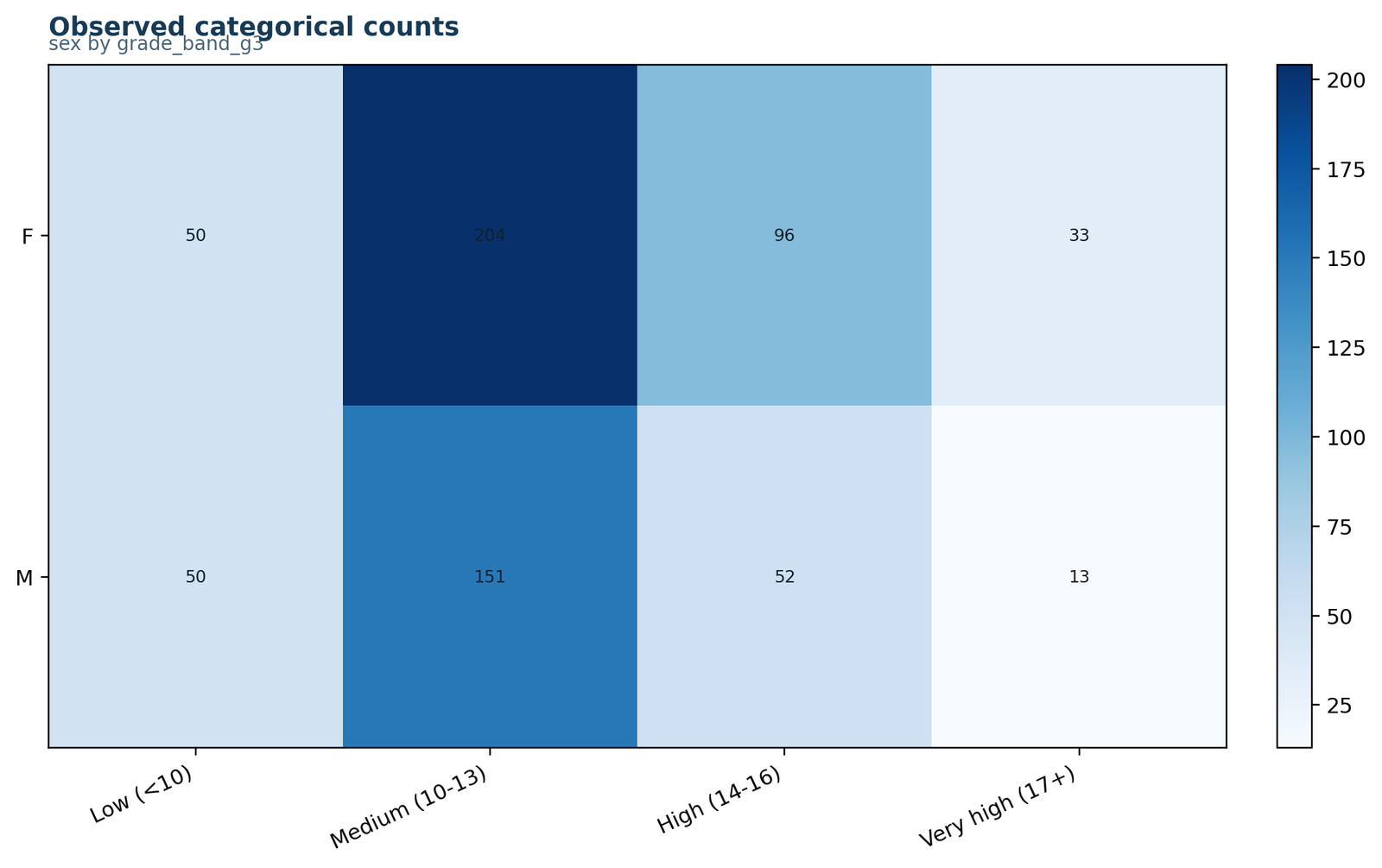
The medium band is the largest category in both rows. The female row contains more observations overall, so raw count comparisons must be paired with within-row percentages.
F: 50, 204, 96 and 33; total 383. M: 50, 151, 52 and 13; total 266.
This is the observed Oij matrix. Every expected count, residual and contribution is derived from these eight cells and their margins.
The equal low-band counts of 50 do not imply equal low-band rates because the row totals differ.
Chart 2: Expected Counts Under IndependencePython and R
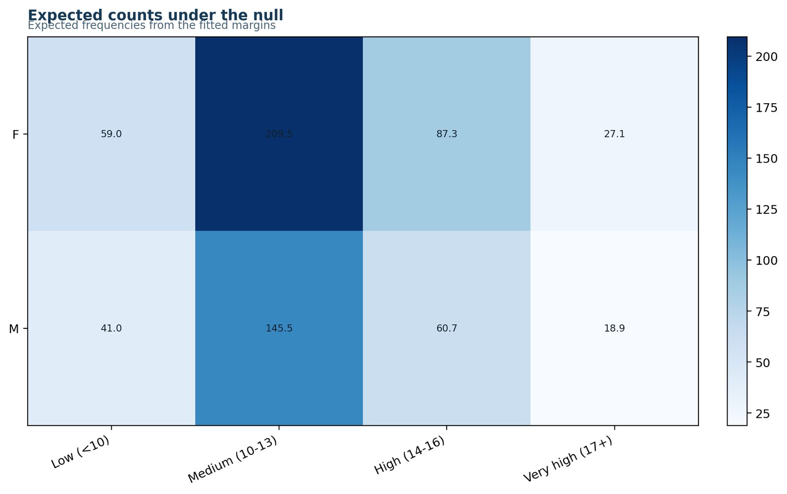
The expected table preserves every observed margin while removing association between the row and column variables.
The smallest expected count is 18.8536 in M | Very high. The largest is 209.4992 in F | Medium.
Observed counts are compared with these values, not with equal counts across all eight cells.
All eight expected counts exceed 5, so the usual asymptotic expected-frequency condition is comfortably satisfied.
Chart 3: Pearson Residual PatternPython and R
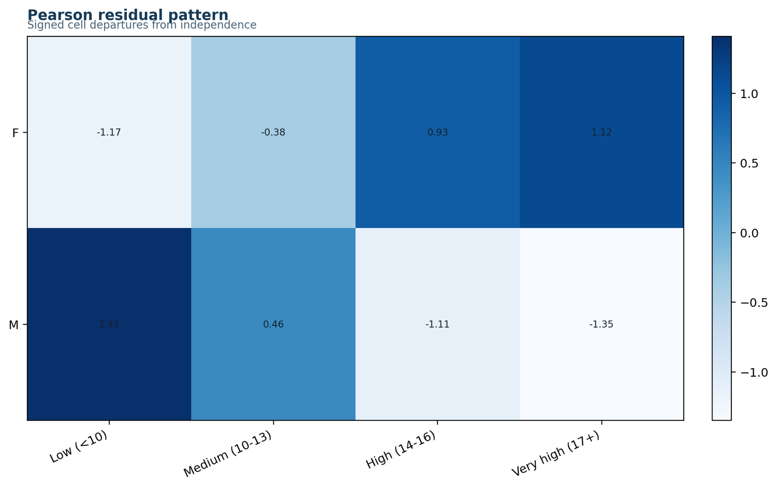
M | Low = 1.4080, M | Medium = 0.4559, F | High = 0.9266 and F | Very high = 1.1235.
F | Low = −1.1734, F | Medium = −0.3799, M | High = −1.1118 and M | Very high = −1.3481.
The rows differ in a coherent direction: the M row is above expectation in lower bands and below expectation in higher bands, with the reverse pattern for F.
No residual exceeds ±2, showing that the significant global result is accumulated across several moderate departures.
Chart 4: Cell Contributions to the Pearson StatisticPython and R
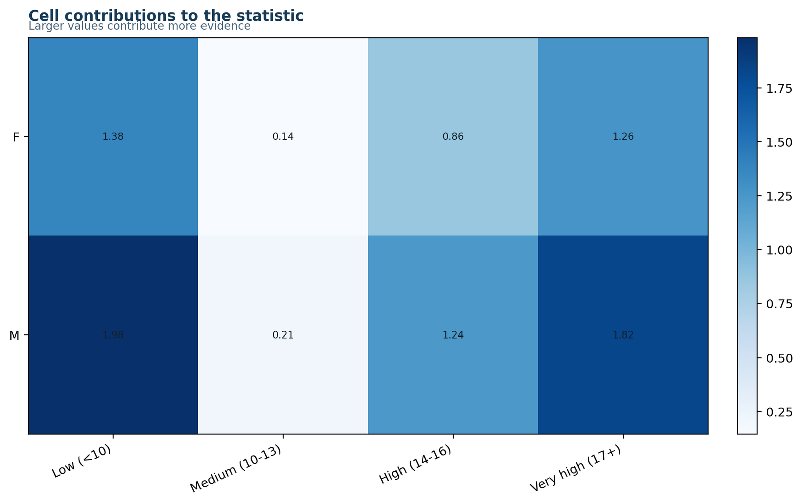
M | Low contributes 1.9824 and M | Very high contributes 1.8174. Together they account for about 42.76% of χ².
F | Low, F | Very high, M | High and F | High contribute between 0.8586 and 1.3768 each.
The two medium-band cells contribute only 0.2078 and 0.1444 despite containing the largest raw counts.
Large raw counts do not necessarily drive the test. Influence depends on the squared difference relative to the expected count.
Chart 5: Python Row-Percentage ComparisonPython
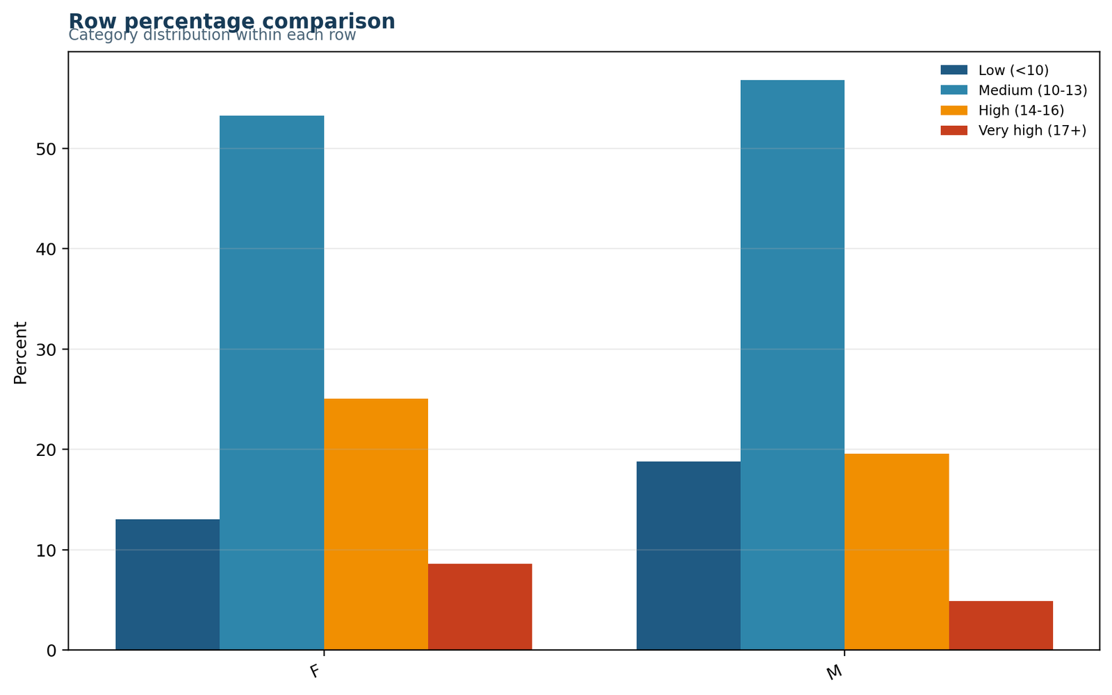
Low 13.05%, medium 53.26%, high 25.07% and very high 8.62%.
Low 18.80%, medium 56.77%, high 19.55% and very high 4.89%.
The largest percentage gaps are in the low, high and very-high categories. The medium profiles are relatively similar.
The percentages are produced by dividing each NumPy or pandas row by its row sum, then multiplying by 100.
Chart 6: Python Model Diagnostics SummaryPython
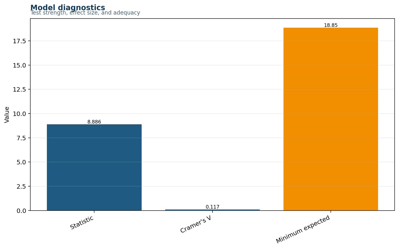
The Pearson statistic is 8.8857 with 3 degrees of freedom and p = 0.030849.
Cramér’s V = 0.1170, which is small in this context.
The minimum expected count is 18.8536, far above 5, and no expected cell is sparse.
The three metrics answer different questions and should not be compared by bar height because they use different scales.
Chart 7: R Row ProfilesR
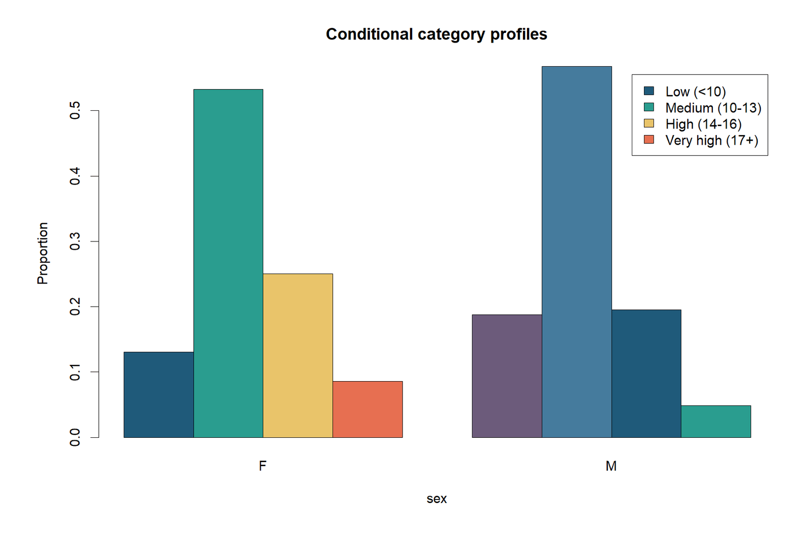
R standardizes each row to a total of 1, making the unequal row sizes directly comparable.
F: .1305, .5326, .2507 and .0862. M: .1880, .5677, .1955 and .0489.
The F row has larger high and very-high shares, whereas the M row has a larger low share.
The R command prop.table(observed, margin = 1) answers the within-row profile question; margin = 2 would answer a different question.
Chart 8: R Result SummaryR
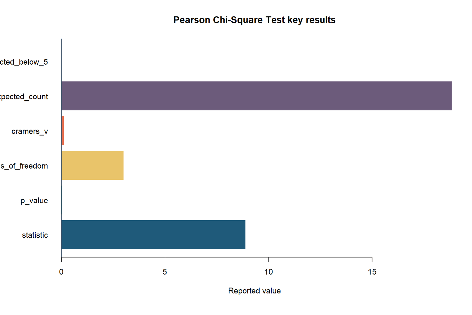
The summary combines inferential, magnitude and adequacy measures without treating them as interchangeable.
χ²: 8.8857; df: 3; p: .03085; V: .1170; minimum expected: 18.8536.
The table is statistically significant, the association is small, and no expected-count warning is present.
A complete result needs all three layers: p-value, effect size and diagnostic adequacy.
Chart 9: R Ranked Cell ContributionsR
The largest bars correspond to M | Low and M | Very high; the medium-band cells contribute least.
M | Low: 1.9824; M | Very high: 1.8174; F | Low: 1.3768; F | Very high: 1.2622.
Contribution ranking identifies influence but not direction. Residual signs are still needed to determine above-versus-below expectation.
Ranking raw counts would be misleading because contribution depends on the squared departure relative to the expected count.
Pearson Chi-Square Test in Python, R, SPSS, Stata and Excel
Pearson Chi-Square Test in Python
Use SciPy’s chi2_contingency for the global test, then calculate residuals, contributions, percentages and Cramér’s V from the returned expected table.
- Pass a two-dimensional integer count array.
- Set
correction=Falsefor the reported Pearson specification. - Verify the returned degrees of freedom equal 3.
- Calculate row percentages from row totals.
- Keep labels in pandas objects when presenting tables.
For broader workflows, see categorical data analysis in Python.
Pearson Chi-Square Test in R
Use chisq.test on a clearly labelled matrix or table. The returned object stores the statistic, p-value, expected counts, Pearson residuals and standardized residuals.
- Set
correct=FALSEfor the 2 × 4 Pearson result. - Use
fit$expectedfor expected counts. - Use
fit$residualsfor Pearson residuals. - Calculate contributions explicitly.
- Use row-wise
prop.tablefor conditional profiles.
See categorical data analysis in R for related table operations.
Pearson Chi-Square Test in SPSS
SPSS CROSSTABS can report observed counts, expected counts, row percentages, Pearson chi-square, likelihood-ratio chi-square, residuals and Cramér’s V.
- Place the two-level variable in rows.
- Place the four-level grade band in columns.
- Request CHISQ and PHI statistics.
- Request COUNT, EXPECTED, ROW, RESID and SRES cells.
- Read the Pearson Chi-Square row, not the likelihood-ratio row, as the primary result.
Pearson Chi-Square Test in Excel
Excel can reproduce the full table calculation with visible formulas. It is especially useful for teaching expected counts and individual cell contributions.
- Enter raw counts, not row percentages.
- Calculate margins with SUM.
- Calculate each expected count from its row and column totals.
- Sum the eight contribution formulas.
- Use CHISQ.DIST.RT for the p-value.
Pearson Chi-Square Test in Stata
Stata’s two-way tabulation command can display counts, row percentages, expected counts and Pearson’s chi-square result.
- Create and label the four-level grade-band variable.
- Use
tabulate rowvar colvar, chi2 expected row. - Confirm Pearson χ² = 8.8857 and df = 3.
- Calculate Cramér’s V separately if needed.
Cross-Software Reconciliation
Python, R, SPSS, Stata and Excel should agree when they use the same eight counts and the uncorrected Pearson formula.
- χ² ≈ 8.885745
- df = 3
- p ≈ 0.030849
- Minimum expected ≈ 18.853621
- Cramér’s V ≈ 0.117010
Expandable Code for the Pearson Chi-Square Test
Python: Pearson test and expected counts
import numpy as np
import pandas as pd
from scipy.stats import chi2_contingency

observed = np.array([
    [50, 204, 96, 33],   # F
    [50, 151, 52, 13]    # M
])

chi2_stat, p_value, dof, expected = chi2_contingency(
    observed,
    correction=False
)

pearson_residuals = (observed - expected) / np.sqrt(expected)
cell_contributions = (observed - expected) ** 2 / expected
row_percentages = observed / observed.sum(axis=1, keepdims=True) * 100

n = observed.sum()
cramers_v = np.sqrt(
    chi2_stat / (n * min(observed.shape[0] - 1,
                         observed.shape[1] - 1))
)

print(f"chi-square = {chi2_stat:.6f}")
print(f"df = {dof}")
print(f"p = {p_value:.8f}")
print(f"Cramer's V = {cramers_v:.6f}")
print(expected)
print(pearson_residuals)
print(cell_contributions)Python: residuals, contributions and Cramér’s V
pearson_residuals = (observed - expected) / np.sqrt(expected)
cell_contributions = (observed - expected) ** 2 / expected
row_percentages = observed / observed.sum(axis=1, keepdims=True) * 100
cramers_v = np.sqrt(chi2_stat / (observed.sum() * min(observed.shape[0]-1, observed.shape[1]-1)))
R: Pearson test and diagnostic objects
observed <- matrix(
  c(50, 204, 96, 33,
    50, 151, 52, 13),
  nrow = 2,
  byrow = TRUE,
  dimnames = list(
    recorded_group = c("F", "M"),
    grade_band_g3 = c(
      "Low (<10)",
      "Medium (10-13)",
      "High (14-16)",
      "Very high (17+)"
    )
  )
)

fit <- chisq.test(observed, correct = FALSE)

expected <- fit$expected
pearson_residuals <- fit$residuals
cell_contributions <- (observed - expected)^2 / expected
row_profiles <- prop.table(observed, margin = 1)

n <- sum(observed)
cramers_v <- sqrt(
  unname(fit$statistic) /
    (n * min(nrow(observed) - 1, ncol(observed) - 1))
)

fit
expected
pearson_residuals
cell_contributions
row_profiles
cramers_vSPSS: CROSSTABS workflow
* Create the four final-grade bands used in this worked example.
RECODE G3
  (LOWEST THRU 9 = 1)
  (10 THRU 13 = 2)
  (14 THRU 16 = 3)
  (17 THRU HIGHEST = 4)
  INTO grade_band_g3.

VALUE LABELS grade_band_g3
  1 'Low (<10)'
  2 'Medium (10-13)'
  3 'High (14-16)'
  4 'Very high (17+)'.

CROSSTABS
  /TABLES = sex BY grade_band_g3
  /FORMAT = AVALUE TABLES
  /STATISTICS = CHISQ PHI
  /CELLS = COUNT EXPECTED ROW RESID SRES
/COUNT ROUND CELL.Stata: two-way tabulation workflow
generate byte grade_band_g3 = .
replace grade_band_g3 = 1 if G3 < 10
replace grade_band_g3 = 2 if inrange(G3, 10, 13)
replace grade_band_g3 = 3 if inrange(G3, 14, 16)
replace grade_band_g3 = 4 if G3 >= 17

label define grade_band_lbl ///
  1 "Low (<10)" ///
  2 "Medium (10-13)" ///
  3 "High (14-16)" ///
  4 "Very high (17+)"
label values grade_band_g3 grade_band_lbl

tabulate sex grade_band_g3, chi2 expected row
Excel: expected counts and contribution formulas
Assume observed counts are in B5:E6, row totals in F5:F6, column totals in B7:E7 and the grand total in F7.
Expected count in B12:
=$F5*B$7/$F$7

Copy B12 across B12:E12 and down through B13:E13.

Cell contribution in B17:
=(B5-B12)^2/B12

Copy B17 across B17:E17 and down through B18:E18.

Pearson statistic:
=SUM(B17:E18)

Degrees of freedom:
=(ROWS(B5:E6)-1)*(COLUMNS(B5:E6)-1)

P-value:
=CHISQ.DIST.RT(Pearson_statistic_cell, Degrees_of_freedom_cell)

Cramer's V:
=SQRT(Pearson_statistic_cell/(F7*MIN(ROWS(B5:E6)-1,COLUMNS(B5:E6)-1)))Assumptions, Limitations and Advanced Interpretation
Core Assumptions
Data Conditions
- Two categorical variables
- Frequency counts rather than percentages
- One cell per observational unit
- Independent observations
- Mutually exclusive categories
- No unexplained structural zeros
Diagnostic Conditions
- Expected counts adequate for the approximation
- Minimum expected count reported
- Sparse-cell percentage checked
- Study design supports the intended inference
- Category definitions fixed before testing
- Effect size reported beside significance
Why “chi-square” does not mean assumption-free
The reference distribution is asymptotic and depends on independent frequency data and an appropriate expected-count structure.
Why independent observations matter
Repeated, matched or clustered observations can make the usual Pearson reference distribution too optimistic. A paired 2 × 2 design requires McNemar’s Test.
Expected-count guidance
Rules vary, but analysts commonly inspect whether any expected count is below 1 and whether more than 20% are below 5. Here every expected count exceeds 18.85.
Structural zeros versus sampling zeros
A sampling zero could have occurred but did not; a structural zero is impossible by design. Structural zeros require a model that respects those constraints.
Why row and column orientation matters
The Pearson statistic is unchanged by transposition, but conditional percentages and the wording of interpretation change.
Why a significant global test does not identify every cell
The alternative requires at least one departure. Residuals and contributions are needed to describe the pattern.
Pearson residuals versus adjusted residuals
Simple Pearson residuals use √E in the denominator. Adjusted residuals account for row and column proportions and are often used for post-hoc cell testing.
Multiple post-hoc comparisons
Testing many cells separately inflates false-positive risk. Prespecify contrasts or use an appropriate multiplicity correction.
Cramér’s V versus statistical significance
The p-value addresses evidence against independence; Cramér’s V addresses standardized magnitude. This analysis is significant but small.
Categorization sensitivity
Changing the G3 cut points changes the contingency table. Thresholds should be substantively justified rather than selected after inspecting p-values.
Clustered observations
If students are nested within schools or classes, a model that accounts for clustering may be required.
Association and causation
The Pearson Chi-Square Test describes association. It does not control confounding or prove that one variable causes the other.
APA Reporting for the Pearson Chi-Square Test
APA reporting should identify the variables, table design, sample size, Pearson statistic, degrees of freedom, p-value, effect size and the principal descriptive pattern.
What to Include in an APA-Style Report
Method Information
- Two categorical variables
- Independent observations
- Table dimensions and category definitions
- Pearson rather than likelihood-ratio statistic
- Expected-count diagnostic
Result Information
- χ² statistic and degrees of freedom
- Sample size
- Exact p-value
- Cramér’s V
- Row percentages and principal cell pattern
APA-Style Methods Sentence
“A Pearson Chi-Square Test of independence was conducted to evaluate the association between recorded F/M group and a four-level G3 grade-band variable.”
Full APA-Style Results Example
“A Pearson Chi-Square Test indicated a statistically significant association between recorded group and G3 grade band, χ²(3, N = 649) = 8.89, p = .031, Cramér’s V = .117. The association was small. The F row contained larger proportions of high and very-high grades, whereas the M row contained a larger low-grade proportion. All expected counts exceeded 18.85.”
Concise APA Results Sentence
“Recorded group and G3 grade band were significantly associated, χ²(3, N = 649) = 8.89, p = .031, Cramér’s V = .117.”
Nonsignificant Pearson Chi-Square Test
Nonsignificant
A Pearson Chi-Square Test did not provide sufficient evidence of an association between row variable and column variable, χ²(df, N = N) = statistic, p = p-value, Cramér’s V = effect size.
Significant Pearson Chi-Square Test
Significant
A Pearson Chi-Square Test showed a statistically significant association between row variable and column variable, χ²(df, N = N) = statistic, p = p-value, Cramér’s V = effect size.
Diagnostic Add-On
Diagnostic
The expected-count condition was satisfied/not satisfied; the minimum expected count was value, and number cells had expected counts below 5.
Reusable APA Templates for the Pearson Chi-Square Test
APA Comparison with the Likelihood-Ratio Test
“Pearson’s chi-square was selected as the primary analysis. The likelihood-ratio chi-square produced the same substantive decision and was treated as a sensitivity comparison rather than a replacement result.”
APA-Style Table for the Main Results
| Statistic or diagnostic | Value | Interpretation |
|---|---|---|
| Pearson χ² | 8.885745 | Global departure from independence |
| Degrees of freedom | 3 | Based on a 2 × 4 table |
| P-value | 0.030849 | Reject H0 at α = .05 |
| Cramér’s V | 0.117010 | Small association |
| Minimum expected count | 18.853621 | Approximation supported |
Suggested table note: “Expected counts were calculated from the observed margins. No expected count was below 5.”
APA Rounding Rules
- Report χ² to two decimals in prose.
- Report p = .031 rather than p = .03 when the exact value is available.
- Use p < .001 rather than p = .000.
- Report Cramér’s V to two or three decimals.
- Retain additional precision in reproducibility tables and workbooks.
APA Interpretation Words to Use
| Avoid | Use instead | Reason |
|---|---|---|
| “The test proved dependence.” | “The test provided evidence of an association.” | Statistical tests do not prove a population claim. |
| “Every category differed.” | “The global table departed from independence.” | The global result does not test each cell separately. |
| “The relationship was strong because p < .05.” | “The association was statistically significant but small.” | Magnitude is described by Cramér’s V. |
Common Pearson Chi-Square Test Mistakes and How to Correct Them
| Mistake | Why it is wrong | Correction |
|---|---|---|
| Entering percentages instead of counts | The expected-frequency model is defined for frequency counts. | Use the original cell counts and report percentages descriptively. |
| Using Pearson correlation for category codes | Numeric labels do not make categories quantitative. | Use the contingency-table Pearson Chi-Square Test. |
| Ignoring dependence | Repeated or clustered observations invalidate the simple independence reference model. | Use a paired, clustered or model-based method. |
| Reading likelihood ratio as Pearson | SPSS displays both statistics in the same table. | Report the Pearson Chi-Square row for the stated analysis. |
| Claiming every cell differs | The global alternative requires only one or more departures. | Inspect residuals and contributions without overgeneralizing. |
| Calling p = .031 a strong association | Significance and magnitude are different concepts. | Report Cramér’s V = .117 and describe it as small. |
| Using df equal to cells minus one | Contingency-table margins constrain independent variation. | Use (rows − 1)(columns − 1). |
| Applying Yates correction to a 2 × 4 table | The familiar continuity correction applies to one-df 2 × 2 settings. | Use the uncorrected Pearson result for this table. |
| Choosing grade cut points after seeing p-values | Outcome-driven categorization inflates false-positive risk. | Prespecify or justify thresholds substantively. |
| Reporting only the p-value | The reader cannot assess pattern, adequacy or magnitude. | Report counts, percentages, expected counts and Cramér’s V. |
Pearson Chi-Square Test Reports and Worked Excel Download
Python PDF Report
Python results, diagnostics and chart output.
SPSS PDF Output
Crosstabs, Pearson statistics, expected counts and association measures.
Worked Excel Analysis
Formula-audited observed table, expected counts, residuals, contributions and reporting sheet.
R Ranked-Contributions Figure
R-specific cell-contribution ranking supplied with the analysis assets.
Frequently Asked Questions About the Pearson Chi-Square Test
The questions below address formula, assumptions, expected counts, software, residuals, effect size, APA reporting and interpretation.
What is the Pearson Chi-Square Test?
It is a categorical-count test that compares observed contingency-table frequencies with the frequencies expected under a specified null model, commonly independence between two categorical variables.
What is Pearson’s chi-square test used for?
It is used for goodness-of-fit, independence and homogeneity questions. The worked analysis uses the independence form for a 2 × 4 contingency table.
What is the Pearson Chi-Square Test formula?
The statistic is χ² = Σ(O − E)²/E, summed over every cell. Each expected count is row total × column total ÷ grand total.
How do I interpret a significant Pearson Chi-Square Test?
A significant result indicates that the complete observed table departs from the null model more than expected by chance under the reference approximation. It does not identify causation or prove that every cell differs.
What are the assumptions of the Pearson Chi-Square Test?
The data should be counts from independent observational units in mutually exclusive categories, with expected frequencies adequate for the chi-square approximation and no unmodelled structural zeros.
Does the Pearson Chi-Square Test require normality?
No. It is a test for categorical counts and does not require normally distributed variables.
How are degrees of freedom calculated?
For an R × C independence table, df = (R − 1)(C − 1). The 2 × 4 worked table has 3 degrees of freedom.
What is the result in the worked example?
The result is χ²(3, N = 649) = 8.885745, p = 0.030849, with Cramér’s V = 0.117010.
What does Cramér’s V = 0.117 mean?
It indicates a small association in this context. The practical interpretation should also consider the row profiles and subject-matter consequences.
Which cells contribute most to the statistic?
M | Low contributes 1.9824 and M | Very high contributes 1.8174, the two largest individual contributions.
Why are the low-band counts both 50 but their percentages different?
The row totals differ. Fifty of 383 is 13.05%, whereas 50 of 266 is 18.80%.
Should I use Fisher’s exact test instead?
Exact testing is especially relevant when expected counts are sparse. Here the minimum expected count is 18.85, so the Pearson approximation is well supported.
Is Pearson chi-square the same as Pearson correlation?
No. Pearson chi-square analyses categorical counts, while Pearson correlation measures linear association between quantitative variables.
How do I run the test in Python?
Use SciPy’s chi2_contingency on the observed count matrix, then calculate residuals, contributions and Cramér’s V separately.
How do I run the test in R?
Use chisq.test on a labelled matrix or table with correct = FALSE for this 2 × 4 analysis. Read the expected and residual components from the returned object.
How do I read the SPSS output?
Read the Pearson Chi-Square row for the statistic, degrees of freedom and p-value; inspect expected counts in the crosstab and Cramér’s V in the symmetric-measures table.
Can Excel calculate the Pearson Chi-Square Test?
Yes. Excel can calculate margins, expected counts, contributions, the total statistic, degrees of freedom, the p-value and Cramér’s V with worksheet formulas.
What should be reported besides the p-value?
Report the table or key counts, row or column percentages, expected-count diagnostic, Pearson statistic, degrees of freedom, sample size, p-value, Cramér’s V and the principal residual or contribution pattern.
What is the expected-count formula?
For each cell, expected count equals row total multiplied by column total and divided by the grand total.
What is the minimum expected count here?
The minimum expected count is 18.853621 in the M | Very high cell.
How many expected cells are below 5?
Zero of the eight expected cells are below 5.
What is the largest Pearson residual?
The largest absolute simple Pearson residual is approximately 1.4080 in M | Low.
What is the largest cell contribution?
M | Low contributes approximately 1.9824 to the total χ² statistic.
Why can a table be significant when no residual exceeds 2?
Several moderate departures can accumulate to produce a significant global statistic even when no single simple residual is extreme.
Is Yates correction used here?
No. This is a 2 × 4 table with 3 degrees of freedom; the familiar Yates correction applies to one-degree-of-freedom 2 × 2 settings.
What is the likelihood-ratio result?
The likelihood-ratio statistic is approximately 9.0078 with 3 degrees of freedom and p = .0292.
Can the test adjust for covariates?
No. Use a suitable categorical regression or log-linear model when adjustment is required.
Can I collapse the four grade bands?
Only when a substantively justified analysis plan supports the collapse. Do not merge categories merely to obtain a smaller p-value.
Does association imply causation?
No. The Pearson Chi-Square Test identifies association under the study design; it does not establish a causal effect.
What is the main conclusion from this worked example?
Recorded group and G3 grade band are statistically associated, but the association is small and the expected-count condition is comfortably satisfied.
Pearson Chi-Square Test Conclusion
The Pearson Chi-Square Test provides a transparent framework for evaluating whether two categorical variables are independent. In the worked 2 × 4 table, the observed frequencies depart significantly from the independence-expected frequencies, χ²(3, N = 649) = 8.89, p = .031. The association is small, Cramér’s V = .117, and the expected-count condition is comfortably satisfied.
The strongest interpretation comes from combining the global test with the row profiles, signed residuals and ranked cell contributions. The male row contains a larger proportion of low grades and a smaller proportion of high and very-high grades, while the female row shows the reverse pattern. The result describes association, not causation, and should be reported with the exact category definitions and study design.
The report should therefore state the categorical design, observed table, χ² statistic, degrees of freedom, p-value, Cramér’s V, expected-count diagnostic and the main residual or contribution pattern without claiming causation.

