
Nonparametric correlation, monotonic association, average ranks and tied-rank correction
Spearman Rank Correlation: Formula, Interpretation, Python, R, SPSS and Excel Guide
Spearman Rank Correlation, also called Spearman rho or Spearman’s rank correlation coefficient, measures the strength and direction of a monotonic association between two variables after converting the original values into ranks. This guide uses a fully worked example with G1 first-period grade and G3 final grade, where rho = 0.8833, n = 649, and p < .001, showing a very strong positive monotonic relationship.
Quick Answer: Spearman Rank Correlation Result
The main Spearman Rank Correlation analysis tests the monotonic association between G1 and G3. G1 is the first-period grade and G3 is the final grade. The analysis uses 649 valid paired cases.
Because the grade variables contain many tied values, the correct Spearman rho is calculated as the Pearson correlation of average ranks. The result is rho = 0.8832876375, with t approximation = 47.9222869, df = 647, and two-tailed p = 4.9873745 × 10-215. The decision at alpha .05 is to reject H0.
Final interpretation: There is a very strong positive monotonic association between G1 and G3. Students with higher first-period grades tend to rank higher on final grades. This is a rank-based association result, not proof of causation.
Tie warning: The classic shortcut formula 1 − 6Σd² / [n(n² − 1)] gives 0.8847457 here, but the preferred result is 0.8832876 because the data contain tied ranks. With ties, Spearman rho should be computed as the Pearson correlation of average ranks.
Table of Contents
- What Is Spearman Rank Correlation?
- When Should You Use Spearman Correlation?
- Spearman vs Pearson Correlation
- Spearman Rank Correlation Formula
- Null and Alternative Hypotheses
- Dataset and Variables Used
- Verified Spearman Result
- Top Pairwise Spearman Correlations
- Spearman Correlation Matrix Interpretation
- Python Chart-by-Chart Interpretation
- R Chart-by-Chart Interpretation
- SPSS Output Interpretation
- Excel Worked Formula Explanation
- Python, R, SPSS and Excel Workflows
- Code Blocks and Excel Formulas
- Assumptions and Diagnostics
- How to Report Spearman Rank Correlation
- Common Mistakes
- Downloads and Resources
- Related Statistical Guides
- FAQs About Spearman Rank Correlation
What Is Spearman Rank Correlation?
Spearman Rank Correlation is a nonparametric correlation method that measures whether two variables move together in a monotonic way. A monotonic relationship means that as one variable increases, the other variable tends to increase or tends to decrease, but the pattern does not need to be perfectly linear.
The coefficient is usually written as ρ, rho, or rs. It ranges from -1 to +1. A value near +1 means the ranks move upward together. A value near -1 means one variable ranks higher when the other ranks lower. A value near 0 means little monotonic association.
In this worked example, G1 and G3 have rho = 0.8833. This means students with higher first-period grades tend to have higher final grades in rank order. The association is very strong and positive.
Spearman correlation is useful when variables are ordinal, not normally distributed, affected by outliers, or monotonic but not strictly linear. It connects naturally with Correlation in Python, Correlation in R, Correlation in SPSS, Correlation in Excel, Correlation Matrix, Correlation Heatmap, Correlation Assumptions, Parametric vs Nonparametric Tests, p-value and effect size.
Simple definition: Spearman Rank Correlation is the Pearson correlation of ranked values. It measures monotonic association rather than raw linear association.
When Should You Use Spearman Correlation?
Use Spearman correlation when the research question is about rank-order association or monotonic relationship. It is often preferred when Pearson correlation assumptions are questionable.
| Situation | Use Spearman? | Reason |
|---|---|---|
| Variables are ordinal | Yes | Spearman works with ranks, so ordinal categories can be analyzed more naturally. |
| Relationship is monotonic but not linear | Yes | Spearman can detect increasing or decreasing rank patterns even when the raw scatter is curved. |
| Data contain outliers | Often useful | Ranks reduce the influence of extreme raw values. |
| Data are strongly skewed | Often useful | Spearman does not require normally distributed raw scores. |
| Both variables are continuous and linear | Pearson may be better | Pearson directly measures raw linear association. |
| You need a nonparametric correlation matrix | Yes | Spearman matrices summarize monotonic relationships across many variables. |
| There are many tied values | Yes, with average ranks | Use average ranks rather than the no-tie shortcut formula. |
In the student performance dataset, many variables are ordinal or tied, such as studytime, failures, health, alcohol-use categories and grade scores. That makes Spearman correlation a useful alternative or companion to Pearson correlation.
Spearman vs Pearson Correlation
Spearman and Pearson correlation both measure association, but they answer different questions. Pearson uses raw values and measures linear association. Spearman uses ranks and measures monotonic association.
| Feature | Pearson Correlation | Spearman Rank Correlation |
|---|---|---|
| Data used | Raw numeric values | Ranks of values |
| Main pattern measured | Linear relationship | Monotonic relationship |
| Outlier sensitivity | More sensitive | Less sensitive because values are ranked |
| Ordinal variables | Use with caution | More appropriate |
| Formula idea | Correlation of raw X and Y | Correlation of rank(X) and rank(Y) |
| Example interpretation | Higher G1 values linearly relate to higher G3 values | Higher G1 ranks relate to higher G3 ranks |
For G1 and G3, both Pearson and Spearman correlations are high because the raw grade relationship is strong and the rank relationship is also strong. Spearman is especially useful here because tied grade values are common and the method explains the rank-order relationship clearly.
Spearman Rank Correlation Formula
The most reliable general definition of Spearman rho is:
With tied ranks, use average ranks. For this guide:
The classic no-tie shortcut formula is:
Where d is the difference between the two ranks for each case. This shortcut is exact only when there are no tied ranks. In this dataset, tied ranks exist because grade scores repeat many times. Therefore, the preferred rho is 0.8832876, not the shortcut value 0.8847457.
| Formula Item | Value in This Example | Interpretation |
|---|---|---|
| X variable | G1 | First-period grade is ranked. |
| Y variable | G3 | Final grade is ranked. |
| n | 649 | Valid paired observations. |
| Σd² | 5,250,964 | Sum of squared rank differences. |
| No-tie shortcut rho | 0.8847457 | Learning formula; not preferred with ties. |
| Average-rank Spearman rho | 0.8832876 | Preferred result because tied ranks are present. |
| t approximation | 47.9223 | Used for approximate significance testing. |
| p-value | 4.987 × 10-215 | Statistically significant; report as p < .001. |
Null and Alternative Hypotheses
The Spearman hypothesis test checks whether the population rank correlation is zero.
| Statement | Hypothesis | Meaning |
|---|---|---|
| Null hypothesis | H0: ρ = 0 | There is no monotonic association between G1 and G3. |
| Alternative hypothesis | H1: ρ ≠ 0 | There is a monotonic association between G1 and G3. |
| Observed result | ρ = 0.8833, p < .001 | Reject H0. |
| Practical conclusion | Very strong positive monotonic association | Higher G1 ranks are associated with higher G3 ranks. |
Decision: The null hypothesis is rejected. There is a very strong positive monotonic association between first-period grade and final grade.
Dataset and Variables Used
The main focus pair is G1 and G3. The workbook and reports also calculate pairwise Spearman correlations across numeric and ordinal variables from the student performance dataset.
| Variable | Role | Meaning | Why It Is Useful for Spearman |
|---|---|---|---|
| G1 | Focus X variable | First-period grade | Ranked to compare with final-grade rank. |
| G3 | Focus Y variable | Final grade | Main outcome in the worked Spearman example. |
| G2 | Pairwise matrix variable | Second-period grade | Strongest pairwise Spearman association with G3. |
| studytime | Ordinal-style variable | Weekly study-time group | Good example of why rank methods are useful. |
| failures | Ordinal/count-like variable | Past class failures | Strong negative rank relationship with grades. |
| Dalc and Walc | Ordinal lifestyle variables | Weekday and weekend alcohol use | Strong positive rank association with each other. |
| Medu and Fedu | Ordinal education variables | Mother and father education | Strong positive rank association with each other. |
Many variables have repeated values, which create tied ranks. The workbook therefore uses average ranks rather than assuming every observation has a unique rank.
Verified Spearman Result
The Excel workbook, R report and SPSS output agree on the core result for the focus pair G1 and G3.
| Result Item | Value | Interpretation |
|---|---|---|
| X variable | G1 | First-period grade. |
| Y variable | G3 | Final grade. |
| Valid paired cases | 649 | All focus-pair observations are valid. |
| Spearman rho | 0.8832876 | Very strong positive monotonic association. |
| Sum of d² | 5,250,964 | Total squared distance between G1 and G3 average ranks. |
| No-tie shortcut rho | 0.8847457 | Shown for learning, but tied ranks make the average-rank result preferred. |
| t approximation | 47.9223 | Approximate test statistic. |
| Degrees of freedom | 647 | n − 2. |
| Two-tailed p-value | 4.987 × 10-215 | Report as p < .001. |
| Decision | Reject H0 | The association is statistically significant. |
| Effect interpretation | Very strong positive | Higher G1 ranks are strongly associated with higher G3 ranks. |
Top Pairwise Spearman Correlations
The pairwise matrix ranks all numeric and ordinal variable pairs by absolute Spearman rho. The strongest pair is G2 vs G3, not the worked G1 vs G3 pair. The worked example uses G1 and G3 because it is simple to explain with ranks and rank differences.
| Rank | Pair | Spearman rho | Direction | Strength | Interpretation |
|---|---|---|---|---|---|
| 1 | G2 vs G3 | 0.9444512 | Positive | Very strong | Second-period grade and final grade have the strongest rank relationship. |
| 2 | G1 vs G2 | 0.8930649 | Positive | Very strong | First-period and second-period grade ranks move together strongly. |
| 3 | G1 vs G3 | 0.8832876 | Positive | Very strong | Focus pair; first-period grade rank strongly matches final-grade rank. |
| 4 | Medu vs Fedu | 0.6471942 | Positive | Strong | Mother and father education ranks are strongly related. |
| 5 | Dalc vs Walc | 0.6130561 | Positive | Strong | Weekday and weekend alcohol-use ranks move together. |
| 6 | failures vs G3 | -0.4483603 | Negative | Moderate | Higher failures rank is associated with lower final-grade rank. |
| 7 | failures vs G2 | -0.4357405 | Negative | Moderate | Past failures are negatively associated with second-period grade rank. |
| 8 | failures vs G1 | -0.4324323 | Negative | Moderate | Past failures are negatively associated with first-period grade rank. |
| 9 | goout vs Walc | 0.3724547 | Positive | Moderate | Going out and weekend alcohol-use ranks move together. |
| 10 | freetime vs goout | 0.3543453 | Positive | Moderate | Free-time rank and going-out rank are moderately associated. |
The top pairwise results show that grade variables dominate the student performance rank structure. Lifestyle and family-background variables also show meaningful monotonic associations, but they are weaker than grade-to-grade relationships.
Spearman Correlation Matrix Interpretation
The Spearman matrix summarizes rank relationships among all selected variables. Positive values show variables that tend to rank high together. Negative values show that high rank on one variable tends to occur with low rank on the other.
| Matrix Pattern | Example | Interpretation |
|---|---|---|
| Strong grade cluster | G1, G2, G3 | Students who rank high in one grade measure tend to rank high in the others. |
| Strong family education relationship | Medu vs Fedu, rho = 0.6472 | Mother and father education ranks are strongly associated. |
| Strong alcohol-use relationship | Dalc vs Walc, rho = 0.6131 | Weekday and weekend alcohol-use ranks move together. |
| Negative academic-risk pattern | failures vs G3, rho = -0.4484 | Higher past-failure rank is associated with lower final-grade rank. |
| Weak study pattern | studytime vs G3, rho = 0.2747 | More studytime is associated with slightly higher final-grade rank. |
| Small attendance relationship | absences vs G3, rho = -0.1585 | More absences are weakly associated with lower final-grade rank. |
Python Chart-by-Chart Interpretation
The Python charts visualize the focus pair, the rank transformation, the Spearman matrix, the rank-difference diagnostic and the strongest pairwise monotonic associations. The Python PDF link was provided as an asset, but the URL returned a 404 during verification, so the interpretations below are grounded in the uploaded Excel workbook, the accessible R report and the chart file names provided for this post.
Python Chart 1: Original Scatterplot with Monotonic Context
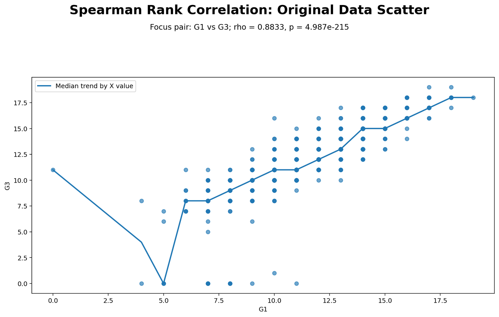
The original scatterplot shows the raw relationship between G1 and G3. The points form a clear upward pattern: students with higher G1 scores generally have higher G3 scores. This supports the very strong positive Spearman result.
The chart is not only about a straight line. Spearman correlation focuses on rank order. Even when many values are tied or repeated, the overall ordering still shows that higher G1 positions are associated with higher G3 positions.
This chart is useful as the first visual because it connects the reader’s intuition to the later rank transformation. Before looking at ranks, the raw scores already suggest a strong increasing relationship.
Python Chart 2: Rank Scatterplot with Equal Rank Line
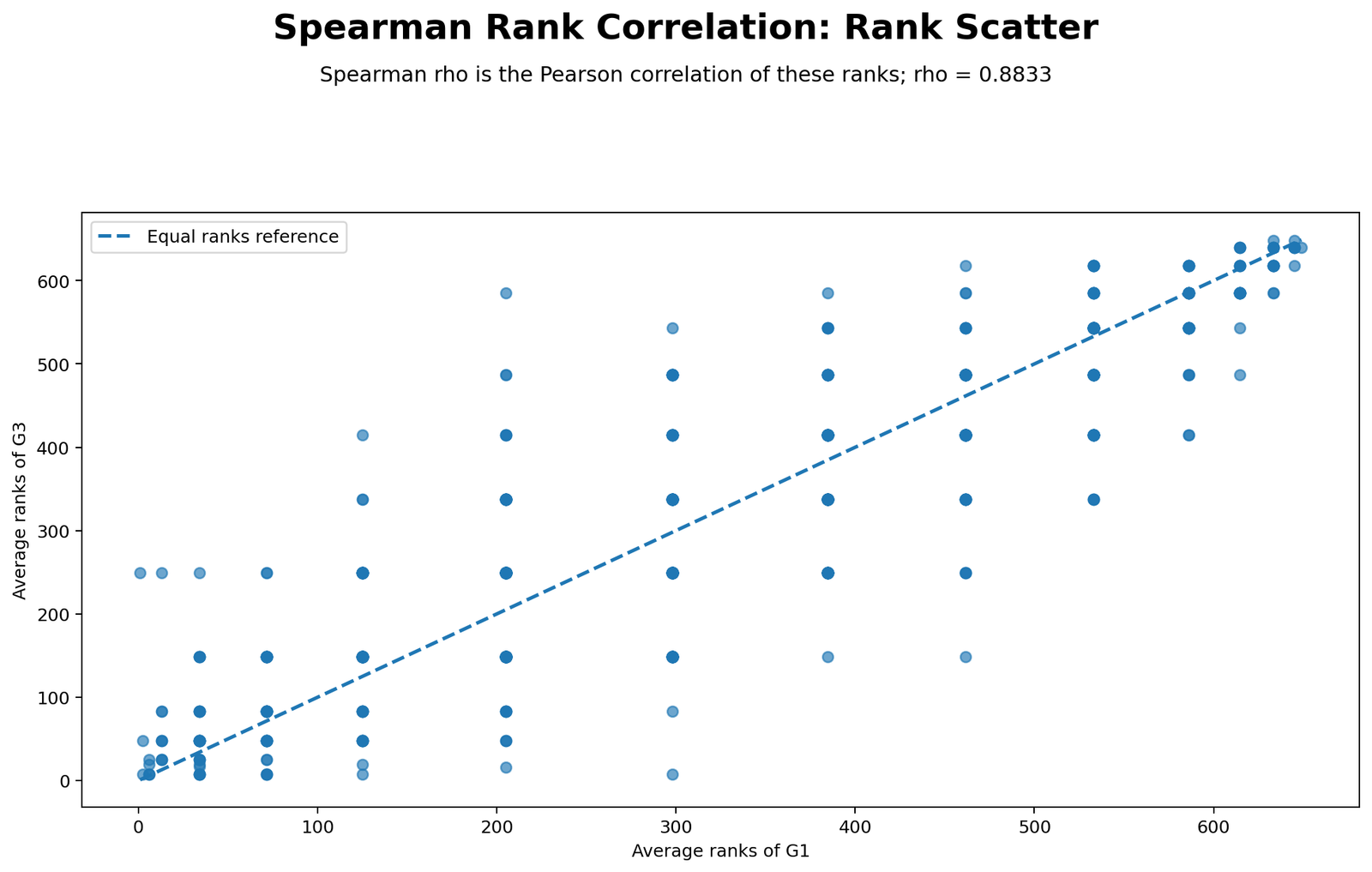
The rank scatterplot is the most important Spearman visual. The x-axis shows average ranks of G1 and the y-axis shows average ranks of G3. The equal-rank reference line helps readers see whether cases keep a similar rank position across the two variables.
Because the points cluster around an upward diagonal pattern, the Spearman rho is very high. The verified result is rho = 0.8833. Cases far from the diagonal represent larger rank disagreement between G1 and G3.
This chart also explains why average ranks matter. Grade values repeat, so tied observations receive averaged rank positions. Spearman rho is then calculated as the Pearson correlation between those average rank columns.
Python Chart 3: Spearman Correlation Matrix Heatmap
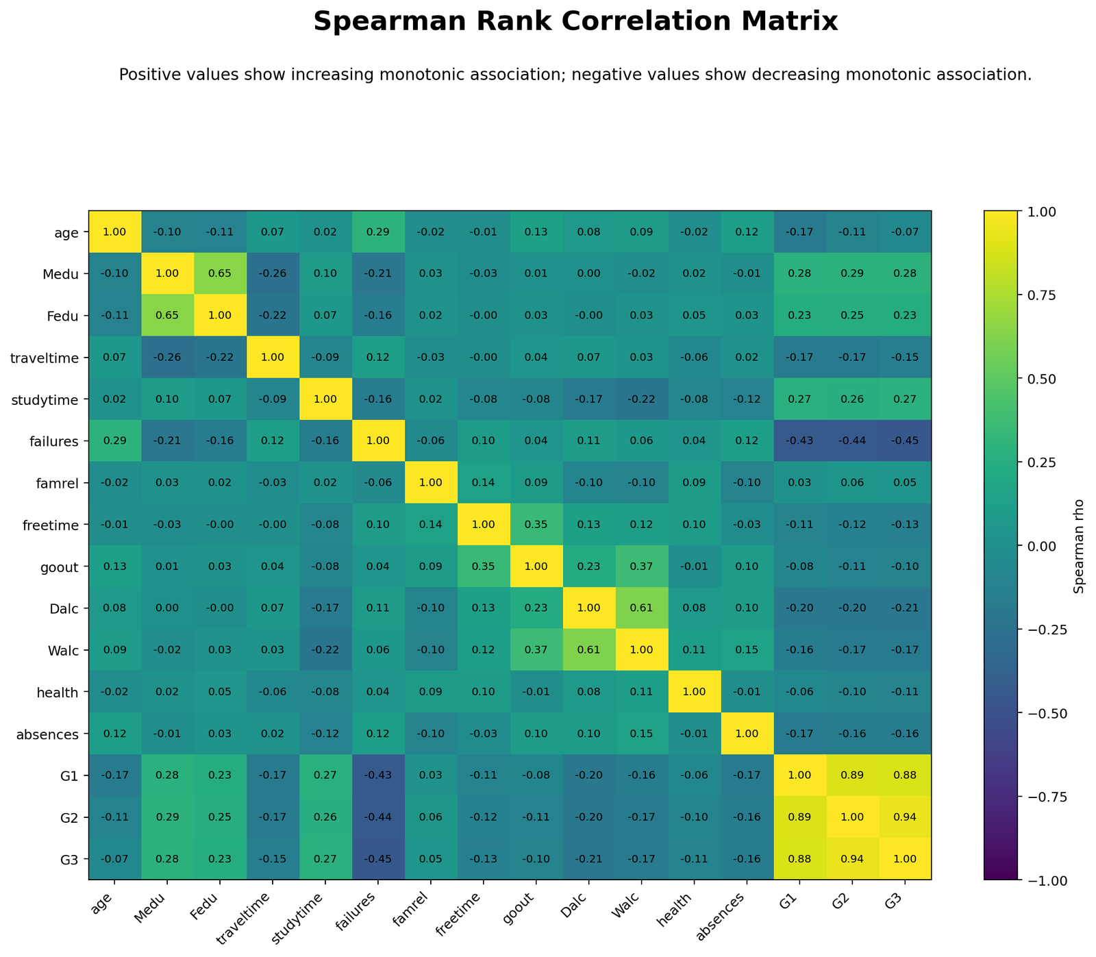
The matrix heatmap shows all rank correlations at once. The strongest positive area appears among G1, G2 and G3. These grade variables rank together strongly, especially G2 and G3 with rho = 0.9445.
The heatmap also shows meaningful positive monotonic relationships between Medu and Fedu and between Dalc and Walc. Negative cells show variables that move in opposite rank directions, such as failures with grade variables.
This chart is helpful for identifying clusters. It shows that academic performance variables form the strongest block, while lifestyle and family variables form weaker but still interpretable patterns.
Python Chart 4: Rank Differences by Case
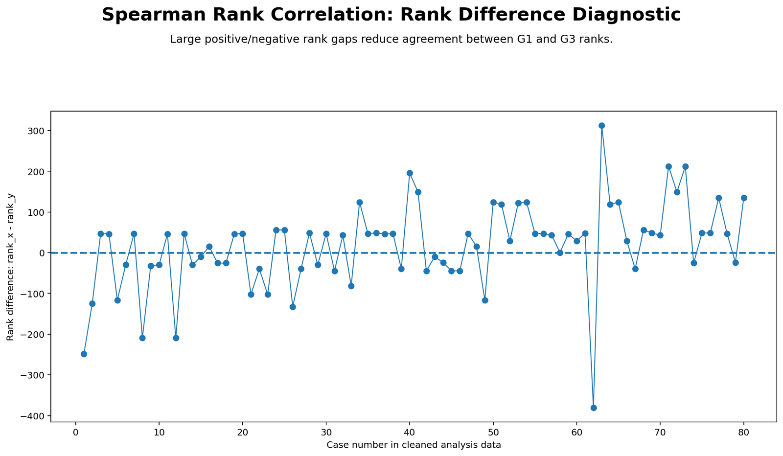
The rank-difference chart shows the difference between each student’s G1 rank and G3 rank. Values near zero mean the student has similar rank positions on both variables. Large positive or negative values show rank disagreement.
The workbook reports Σd² = 5,250,964. This value is used in the classic no-tie formula and is also useful for teaching how rank gaps reduce perfect rank agreement.
This chart gives the most concrete explanation of why rho is below 1.00. The association is very strong, but not perfect, because some students rank much higher in G1 than G3 or much higher in G3 than G1.
Python Chart 5: Top Pairwise Spearman Correlations
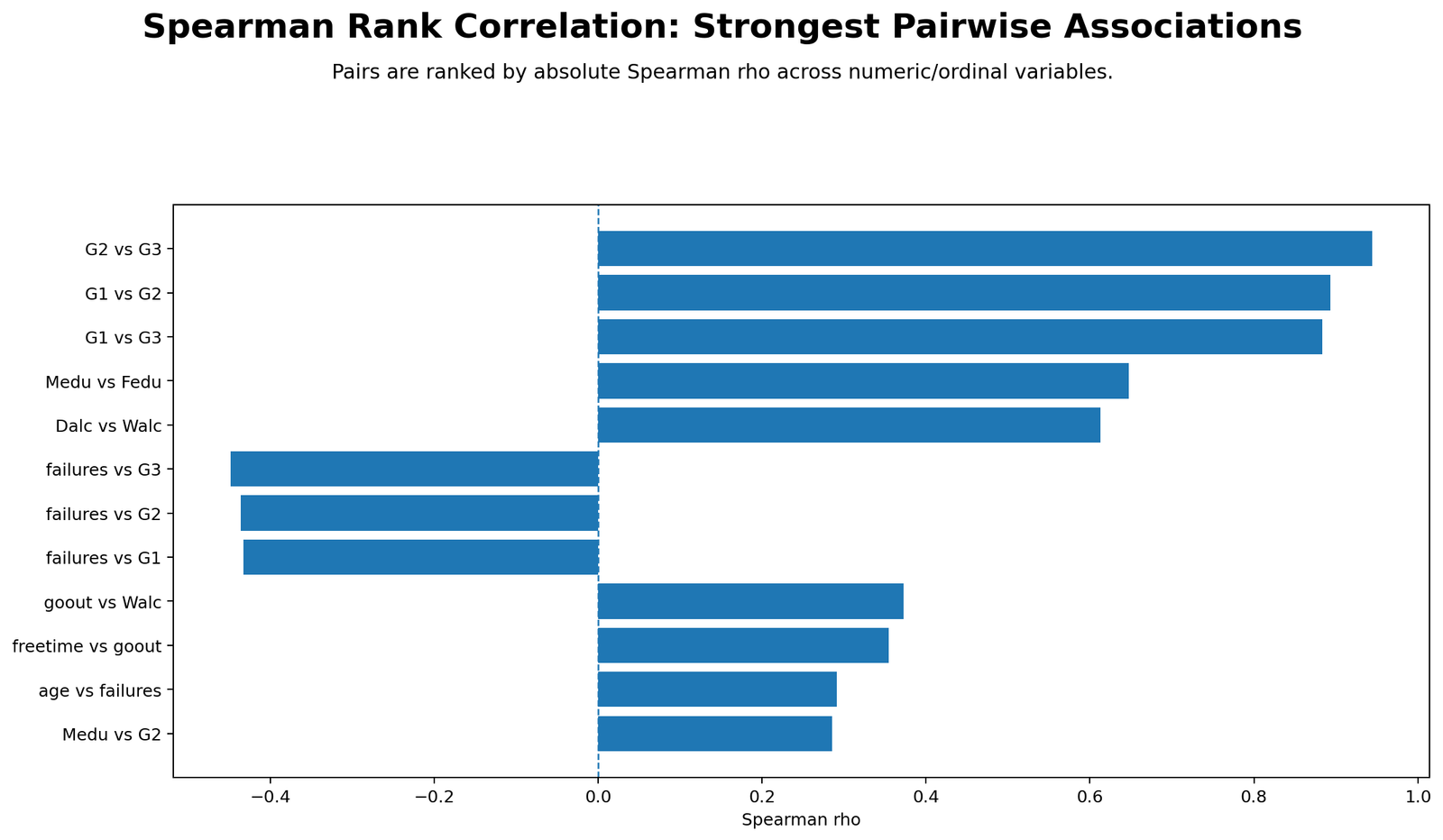
The top-pair chart ranks the strongest monotonic associations in the dataset. The top three are G2 vs G3, G1 vs G2 and G1 vs G3. This confirms that grade variables dominate the rank-order structure.
The chart also includes positive non-grade relationships such as Medu vs Fedu and Dalc vs Walc, plus negative academic-risk relationships involving failures and grades.
This chart is useful for a report because it reduces the large matrix into a ranked summary. Instead of reading every cell, readers can immediately see which monotonic relationships are strongest.
R Chart-by-Chart Interpretation
The R report validates the same result and includes colorful versions of the Spearman charts. The R output confirms the focus pair G1 vs G3, n = 649, rho = 0.8832876, t approximation = 47.92229, df = 647, and p = 4.987375e-215.
R Chart 1: Colorful Original Scatterplot

The R original scatterplot confirms the same increasing pattern between G1 and G3. Higher first-period grades tend to align with higher final grades.
This chart supports the monotonic interpretation visually before ranks are introduced. It shows the same story as the Python original scatterplot using a separate software workflow.
R Chart 2: Colorful Rank Scatterplot

The R rank scatterplot displays the actual ranked values used in the Spearman calculation. The upward diagonal pattern confirms a very strong positive rank relationship.
This is the best R chart for explaining the coefficient. Spearman rho is not mysterious: it is simply the correlation of these rank columns when tied values are handled with average ranks.
R Chart 3: Colorful Spearman Matrix Heatmap

The R heatmap validates the same rank-correlation matrix. Grade variables show the strongest positive cluster, failures show negative grade relationships, and Dalc–Walc plus Medu–Fedu show strong positive monotonic associations.
Using both Python and R matrices is useful because it shows that the findings are not software-specific. The same rank relationships appear across workflows.
R Chart 4: Colorful Rank Differences by Case

The R rank-difference chart shows where G1 and G3 ranks disagree. Large positive or negative rank gaps reduce the coefficient, while near-zero gaps support high rank agreement.
Because rho is still very high, most rank positions are broadly aligned. However, the diagnostic chart makes clear that the relationship is not perfect.
R Chart 5: Colorful Top Pairwise Spearman Correlations

The R top-pairs chart highlights the same strongest monotonic relationships: G2–G3, G1–G2, G1–G3, Medu–Fedu and Dalc–Walc.
The negative failure-grade relationships are also important. They show that students with higher ranks on past failures tend to rank lower on grade outcomes.
SPSS Output Interpretation
The SPSS output confirms the focus-pair result using SPSS nonparametric correlations. SPSS reports the G1–G3 Spearman coefficient as approximately .883, with Sig. (2-tailed) = .000 and N = 649. In report writing, SPSS .000 should be written as p < .001, not p = .000.
Open the SPSS Spearman Rank Correlation output PDF
| SPSS Output Item | Value | Interpretation |
|---|---|---|
| Procedure | Nonparametric Correlations | Spearman’s rho selected for G1 and G3. |
| Focus pair | G1 and G3 | First-period grade and final grade. |
| Correlation coefficient | .883 | Very strong positive Spearman association. |
| Sig. (2-tailed) | .000 | Report as p < .001. |
| N | 649 | Valid paired observations. |
| Rank construction | Mean ranks for tied values | SPSS uses average ranks for ties. |
| Pearson correlation of ranks | .883 | Confirms Spearman rho as correlation of average ranks. |
The SPSS output is useful for students because it shows both the nonparametric correlation table and a manual rank-construction section. This proves the method: rank G1, rank G3, use average ranks for ties, and correlate the rank columns.
Excel Worked Formula Explanation
The uploaded Excel workbook provides a fully worked Spearman Rank Correlation analysis. It includes the dataset, rank working sheet, final report, pairwise matrix and top pairwise results.
| Excel Sheet | Purpose | What It Teaches |
|---|---|---|
| ReadMe | Explains the workbook purpose and key values. | Shows focus variables, n, rho, p-value, tie note and reporting guidance. |
| Dataset | Stores the embedded dataset. | Keeps the analysis self-contained. |
| Spearman_Working | Shows original values, average ranks, rank differences and squared differences. | Provides the fully worked rank calculation. |
| Report | Summarizes the final G1–G3 result. | Shows rho, t approximation, df, p-value, decision and report sentence. |
| Pairwise_Matrix | Static Spearman matrix across selected variables. | Shows monotonic relationships among all numeric and ordinal variables. |
| Top_Pairwise | Ranks strongest absolute Spearman correlations. | Highlights strongest positive and negative monotonic associations. |
Excel Formula Method
The workbook uses RANK.AVG for tied ranks and CORREL to calculate Spearman rho as the correlation of average ranks.
| Step | Excel Formula Pattern | Purpose |
|---|---|---|
| Rank X values | =RANK.AVG(B9,$B$9:$B$657,1) | Ranks G1 in ascending order using average ranks for ties. |
| Rank Y values | =RANK.AVG(C9,$C$9:$C$657,1) | Ranks G3 in ascending order using average ranks for ties. |
| Rank difference | =D9-E9 | Finds the difference between G1 rank and G3 rank. |
| Squared rank difference | =F9^2 | Used for the classic no-tie shortcut formula. |
| Preferred Spearman rho | =CORREL(rank_G1_range,rank_G3_range) | Correct tied-rank Spearman result. |
| Classic no-tie rho | =1-(6*SUM(d_squared_range))/(n*(n^2-1)) | Learning formula, exact only without ties. |
| t approximation | =rho*SQRT((n-2)/(1-rho^2)) | Approximate test statistic. |
| Two-tailed p-value | =T.DIST.2T(ABS(t),df) | Approximate significance value. |
In the workbook, the first few working rows show how ranks can differ sharply. For example, one case has G1 = 0 and G3 = 11, producing rank G1 = 1 and rank G3 = 249.5, so the rank difference is -248.5. These large rank gaps explain why rho is less than 1, even though the association is very strong.
Python, R, SPSS and Excel Workflows
Spearman Rank Correlation can be calculated in Python, R, SPSS and Excel. The key is to use the same variables, missing-value rule and tied-rank method.
| Software | Main Workflow | Best Use |
|---|---|---|
| Python | Use pandas for data preparation, scipy.stats.spearmanr for rho and p-value, and matplotlib for rank scatterplots and heatmaps. | Automated charts and reproducible reporting. |
| R | Use cor.test(…, method = “spearman”) and rank(…, ties.method = “average”) for manual verification. | Statistical validation and colorful charts. |
| SPSS | Use Analyze → Correlate → Bivariate or Nonparametric Correlations, select Spearman, and report rho, p and N. | Formal output for assignments, thesis and research reports. |
| Excel | Use RANK.AVG, CORREL, rank differences and T.DIST.2T formulas. | Fully worked formula teaching and transparent verification. |
Code Blocks and Excel Formulas
Python Code for Spearman Rank Correlation
import pandas as pd
from scipy import stats

df = pd.read_csv("dataset.csv")

x_var = "G1"
y_var = "G3"

work = df[[x_var, y_var]].dropna().copy()
work[x_var] = pd.to_numeric(work[x_var], errors="coerce")
work[y_var] = pd.to_numeric(work[y_var], errors="coerce")
work = work.dropna()

rho, p_value = stats.spearmanr(work[x_var], work[y_var])
n = len(work)

t_approx = rho * ((n - 2) / (1 - rho**2)) ** 0.5
dfree = n - 2

print("X variable:", x_var)
print("Y variable:", y_var)
print("N:", n)
print("Spearman rho:", rho)
print("t approximation:", t_approx)
print("df:", dfree)
print("p-value:", p_value)
Python Code for Manual Average-Rank Check
import pandas as pd
from scipy import stats

df = pd.read_csv("dataset.csv")
work = df[["G1", "G3"]].dropna().copy()

work["rank_G1"] = work["G1"].rank(method="average", ascending=True)
work["rank_G3"] = work["G3"].rank(method="average", ascending=True)
work["d"] = work["rank_G1"] - work["rank_G3"]
work["d_squared"] = work["d"] ** 2

rho_from_ranks, p_from_ranks = stats.pearsonr(work["rank_G1"], work["rank_G3"])

n = len(work)
classic_no_tie_rho = 1 - (6 * work["d_squared"].sum()) / (n * (n**2 - 1))

print("Spearman rho as Pearson correlation of average ranks:", rho_from_ranks)
print("Sum d squared:", work["d_squared"].sum())
print("Classic no-tie formula rho:", classic_no_tie_rho)
print("Note: no-tie formula is exact only when there are no tied ranks.")
R Code for Spearman Rank Correlation
df <- read.csv("dataset.csv", stringsAsFactors = FALSE)

work <- na.omit(df[, c("G1", "G3")])
work$G1 <- as.numeric(work$G1)
work$G3 <- as.numeric(work$G3)

test <- cor.test(work$G1, work$G3, method = "spearman", exact = FALSE)

print(test)

rank_G1 <- rank(work$G1, ties.method = "average")
rank_G3 <- rank(work$G3, ties.method = "average")

rho_from_ranks <- cor(rank_G1, rank_G3, method = "pearson")
d <- rank_G1 - rank_G3
sum_d_squared <- sum(d^2)

n <- nrow(work)
classic_no_tie_rho <- 1 - (6 * sum_d_squared) / (n * (n^2 - 1))

cat("rho from average ranks:", rho_from_ranks, "\n")
cat("sum d squared:", sum_d_squared, "\n")
cat("classic no-tie formula rho:", classic_no_tie_rho, "\n")
SPSS Syntax for Spearman Rank Correlation
* Spearman Rank Correlation in SPSS.
OUTPUT CLOSE ALL.
OUTPUT NEW NAME=Spearman_Rank_Correlation_Output.

DESCRIPTIVES VARIABLES=G1 G3
  /STATISTICS=MEAN STDDEV MIN MAX.

NONPAR CORR
  /VARIABLES=G1 G3
  /PRINT=SPEARMAN TWOTAIL
  /MISSING=PAIRWISE.

* Manual rank construction for fully worked output.
RANK VARIABLES=G1 G3 (A)
  /RANK
  /PRINT=YES
  /TIES=MEAN.

COMPUTE rank_difference = RG1 - RG3.
COMPUTE rank_difference_squared = rank_difference ** 2.
EXECUTE.

CORRELATIONS
  /VARIABLES=RG1 RG3
  /PRINT=TWOTAIL
  /MISSING=PAIRWISE.

GRAPH
  /SCATTERPLOT(BIVAR)=G1 WITH G3
  /TITLE='Spearman Rank Correlation: Original Values'.

GRAPH
  /SCATTERPLOT(BIVAR)=RG1 WITH RG3
  /TITLE='Spearman Rank Correlation: Average Ranks'.

OUTPUT EXPORT
  /CONTENTS EXPORT=VISIBLE
  /PDF DOCUMENTFILE='Spearman-Rank-Correlation-SPSS-Output.pdf'.
Excel Formula Patterns
Assume:
X_range = G1 values
Y_range = G3 values

Rank G1 with average ranks:
=RANK.AVG(B9,$B$9:$B$657,1)

Rank G3 with average ranks:
=RANK.AVG(C9,$C$9:$C$657,1)

Rank difference:
=rank_G1-rank_G3

Squared rank difference:
=rank_difference^2

Preferred Spearman rho with tied ranks:
=CORREL(rank_G1_range,rank_G3_range)

Classic no-tie shortcut:
=1-(6*SUM(d_squared_range))/(n*(n^2-1))

t approximation:
=rho*SQRT((n-2)/(1-rho^2))

Degrees of freedom:
=n-2

Two-tailed p-value:
=T.DIST.2T(ABS(t),df)

Decision:
=IF(p_value<0.05,"Reject H0","Fail to reject H0")
Assumptions and Diagnostics
Spearman correlation has fewer assumptions than Pearson correlation, but it still needs thoughtful checking.
| Assumption / Check | Meaning | How It Applies Here |
|---|---|---|
| Variables are at least ordinal | Spearman uses ranks, so values should be orderable. | Grades and ordinal-coded variables can be ranked. |
| Paired observations | Each X value must match the correct Y value. | Each student has a G1 and G3 value. |
| Monotonic relationship | As one variable increases, the other tends to increase or decrease. | G1 and G3 show a strong increasing monotonic pattern. |
| Independence of observations | Rows should represent independent cases. | Each row should represent a separate student. |
| Tied ranks handled properly | Repeated values should receive average ranks. | The workbook and SPSS output use average ranks for tied grade values. |
| Outliers reviewed | Spearman is less sensitive than Pearson but still benefits from visual checks. | Original scatterplots and rank-difference charts show unusual rank gaps. |
Spearman is not a free replacement for every correlation problem. It measures monotonic rank association. If the relationship is random or non-monotonic, Spearman rho can still be small even when a complex nonlinear pattern exists.
How to Report Spearman Rank Correlation
A complete Spearman report should include the variables, sample size, rho, p-value, direction, strength and tie handling if relevant.
APA-style report: A Spearman rank-order correlation was computed to examine the monotonic association between G1 first-period grade and G3 final grade. There was a very strong positive monotonic association between G1 and G3, ρ = .883, n = 649, p < .001. Students with higher G1 ranks tended to have higher G3 ranks. Average ranks were used because tied grade values were present.
Short report: Spearman’s rho showed a very strong positive association between G1 and G3, ρ = .883, n = 649, p < .001.
Matrix report: The strongest pairwise Spearman correlation was between G2 and G3, ρ = .944, followed by G1 and G2, ρ = .893, and G1 and G3, ρ = .883. Failures had the strongest negative association with G3, ρ = -.448.
Common Mistakes in Spearman Correlation Interpretation
| Mistake | Why It Is a Problem | Better Practice |
|---|---|---|
| Using the no-tie shortcut with tied data | The shortcut formula is exact only without ties. | Use average ranks and correlate the rank columns. |
| Calling Spearman a linear correlation | Spearman measures monotonic rank association, not raw linear association. | Use “monotonic association” in reporting. |
| Reporting p = .000 from SPSS | p-values should not be reported as exactly zero. | Write p < .001. |
| Ignoring direction | Positive and negative rho values have different meanings. | Explain whether higher ranks move together or opposite. |
| Interpreting correlation as causation | Spearman is an association measure. | Use “associated with,” not “caused by.” |
| Skipping visual checks | A coefficient alone hides rank gaps and monotonic pattern shape. | Use original scatterplots, rank scatterplots and rank-difference diagnostics. |
| Confusing Spearman and Pearson | They use different data transformations and assumptions. | Use Pearson for raw linear association and Spearman for rank monotonic association. |
| Ignoring sample size | Large samples can make even weak rho values significant. | Report strength and p-value together. |
Downloads and Resources
Download R Report PDFR validation report with focus result, variable summary, pairwise results and colorful charts.
Download SPSS Output PDFSPSS nonparametric correlation output and manual rank construction.
External References
For additional learning, review statistical documentation on Spearman’s rho, rank-order correlation, monotonic association, tied ranks, nonparametric correlation tests and correlation matrix interpretation.
FAQs About Spearman Rank Correlation
What is Spearman Rank Correlation?
Spearman Rank Correlation is a nonparametric measure of monotonic association between two variables. It is calculated by ranking both variables and correlating the ranks.
What is the main result in this guide?
The main result is the Spearman correlation between G1 and G3: rho = 0.8832876, n = 649, p < .001. This indicates a very strong positive monotonic association.
Why is the average-rank result preferred?
The dataset contains tied grade values. With tied ranks, Spearman rho should be calculated as the Pearson correlation of average ranks. The classic no-tie shortcut is shown for learning only.
What does a positive Spearman rho mean?
A positive rho means that higher ranks on one variable tend to occur with higher ranks on the other variable. Here, higher G1 ranks tend to occur with higher G3 ranks.
What was the strongest pairwise Spearman correlation?
The strongest pairwise Spearman correlation was G2 vs G3, rho = 0.9444512. This is a very strong positive monotonic association.
What was the strongest negative Spearman correlation with G3?
The strongest negative relationship with G3 was failures vs G3, rho = -0.4483603. Students with higher ranks on past failures tended to rank lower on final grade.
Is Spearman correlation the same as Pearson correlation?
No. Pearson correlation uses raw values and measures linear association. Spearman correlation uses ranked values and measures monotonic association.
Can Excel calculate Spearman correlation?
Yes. Excel can calculate Spearman correlation by using RANK.AVG to create rank columns and then using CORREL on the two rank columns.
How do I report SPSS p = .000?
Report it as p < .001. Do not write p = .000 because the p-value is very small, not exactly zero.
Does Spearman correlation prove causation?
No. Spearman correlation measures association in ranks. It does not prove that one variable causes another.

