
Categorical Data Analysis in Python: Complete Guide with Code, Charts and Interpretation
Categorical data analysis in Python turns labels such as school, region, treatment group, outcome class and survey response into reproducible frequency tables, contingency tables, statistical tests, effect sizes and diagnostic plots. This guide teaches the complete workflow with pandas, NumPy, SciPy and matplotlib, using a verified 649-student example that compares school with four final-grade categories.
2 × 4 contingency table
Pearson χ²(3) = 59.534
p = 7.39 × 10⁻¹³
Cramer's V = 0.303
Categorical Data Analysis in Python Model Overview
What Categorical Data Analysis Does
Categorical data analysis in Python summarizes variables whose values represent groups or classes rather than continuous quantities. The workflow begins with category definitions and frequencies, then moves to cross-tabulation, expected counts, association tests, effect sizes and cell-level diagnostics.
The worked analysis uses school as a two-category explanatory variable and a derived G3 grade band as a four-category outcome. The observed table contains 649 complete records.
Worked Research Question
Is the distribution of final-grade categories the same at the GP and MS schools, or is school statistically associated with the four-level G3 grade band?
Core Python Objects
A pandas DataFrame stores the records. A pandas crosstab stores observed counts. SciPy calculates chi-square and likelihood-ratio tests. NumPy supports residuals and effect sizes. Matplotlib produces interpretable publication charts.
Primary Statistical Result
Pearson's chi-square is 59.534045 with 3 degrees of freedom and p = 7.392e-13. The null hypothesis of independence is rejected.
Practical Magnitude
Cramer's V is 0.302873, indicating a meaningful association. The strongest pattern is the large excess of Low grades at MS and the corresponding shortage at GP.
What a Complete Python Workflow Includes
Clean category labels, define ordered categories, handle missing values and preserve transparent coding.
Calculate frequencies, valid percentages, row percentages, column percentages and visual profiles.
Run Pearson chi-square, likelihood-ratio tests and an exact conditional alternative when required.
Measure association with Cramer's V and the contingency coefficient rather than relying on p-values alone.
Inspect expected counts, Pearson residuals, adjusted residuals and cell contributions.
Combine the test, effect size, important cells, uncertainty and limitations in a reproducible report.
Quick Answer: Categorical Data Analysis in Python Result
Statistical Decision
- Test: Pearson chi-square test of independence.
- Table: school × G3 grade band.
- Result: χ²(3) = 59.534, p < .001.
- Decision: reject independence.
- Effect: Cramer's V = 0.303.
Substantive Interpretation
- GP Low: 32 observed versus 65.2 expected.
- MS Low: 68 observed versus 34.8 expected.
- MS Low contributes 53.1% of the total chi-square.
- No expected cell is below 5.
- The exact conditional result confirms the same conclusion.
Table of Contents
- What is categorical data analysis in Python?
- Types of categorical variables
- Research question and hypotheses
- Data preparation and category coding
- Variables and data dictionary
- Observed contingency table
- Selecting a categorical method
- Complete statistical results
- Expected counts and assumptions
- Residuals and cell contributions
What Is Categorical Data Analysis in Python?
Definition
Categorical data analysis in Python is the process of organizing, visualizing and modelling variables whose values identify categories. Examples include yes/no outcomes, school type, treatment arm, region, occupation, satisfaction level and disease class.
Unlike a continuous variable, a category label does not automatically have meaningful arithmetic. Analysis therefore focuses on counts, proportions, conditional distributions, odds, association and prediction.
Why Python Is Useful
Python combines data cleaning, statistical calculation, plotting and reporting in one reproducible workflow. The same script can read raw data, create derived categories, calculate tables, validate assumptions, produce charts and export results without manual copying.
The most useful libraries are pandas for tables, NumPy for arrays, SciPy for tests and matplotlib for publication figures.
Questions Categorical Data Analysis Can Answer
Distribution Question
How many observations belong to each category, and what percentage of valid cases does each category represent?
Association Question
Does the distribution of one categorical variable differ across the categories of another variable?
Prediction Question
How does a set of predictors change the probability of a binary, nominal or ordinal outcome?
Descriptive and Inferential Layers
The descriptive layer contains frequency tables, cross-tabulations and percentages. The inferential layer tests whether the observed pattern is compatible with a null model. The diagnostic layer identifies which cells create the result, while the effect-size layer describes the magnitude of association.
Why Categorical Data Analysis Is More Than a Chi-Square Test
A chi-square p-value answers one narrow question: whether a table departs from independence more than expected by chance under the model. A complete analysis also checks data coding, category order, missingness, expected frequencies, effect size, residuals, influential cells and practical interpretation.
Types of Categorical Variables in Python
Binary
Exactly two categories, such as Pass/Fail or Yes/No. Binary outcomes support proportions, odds ratios and logistic models.
Nominal
Three or more unordered categories, such as school, region or occupation. Category order has no quantitative meaning.
Ordinal
Ordered categories, such as Low, Medium and High. Order matters, but category distances are not automatically equal.
Count-Derived Category
A quantitative variable can be grouped into bands. The cutpoints must be justified because grouping discards information.
Worked Variable Types
school is nominal with GP and MS categories. grade_band_g3 is ordinal with Low, Medium, High and Very high categories. Pearson chi-square uses the table as categorical and does not exploit the order of the grade bands. The order is used later for substantive interpretation.
Pandas Category Dtype
Using a pandas categorical dtype preserves the intended order, prevents accidental alphabetical sorting and makes chart labels reproducible. Ordered categories are especially important when Low, Medium, High and Very high must appear in a logical sequence.
Do Not Confuse Codes With Quantities
Codes such as 0, 1, 2 and 3 may represent category labels, but their numerical spacing is not automatically meaningful. The analysis should use labels and explicitly declared order rather than treating arbitrary codes as continuous measurements.
See Variables in Statistics for additional distinctions among categorical, quantitative, explanatory and response variables.
Research Question, Hypotheses and Study Design
Research Question
Is final-grade category associated with school, or do GP and MS students have the same G3 grade-band distribution?
Null Hypothesis
School and G3 grade band are independent. Every school's category proportions equal the overall category proportions.
Alternative Hypothesis
School and G3 grade band are associated. At least one school-category cell departs from independence.
Observed Units
The dataset contains 649 student records. Each student contributes to one school row and one G3 grade-band column. The test assumes that records are independent; repeated measurements or clustered sampling require a method that accounts for dependence.
Table Dimensions and Degrees of Freedom
The table has two school rows and four grade-band columns. The degrees of freedom count the number of independent departures possible after row and column margins are fixed.
Why the Worked Analysis Uses Four Grade Bands
The four categories distinguish failing or low performance, middle performance, high performance and very high performance. This retains more outcome detail than a binary pass/fail split, although it still simplifies the original G3 scale.
Data Preparation and Category Coding in Python
Cleaning Category Labels
Strip leading and trailing spaces, standardize capitalization, convert empty strings to missing values and inspect unexpected labels before building tables. Two visually similar labels such as “GP” and “GP ” otherwise become separate categories.
Creating the G3 Grade Band
The verified cutpoints are Low below 10, Medium from 10 through 13, High from 14 through 16, and Very high at 17 or above. The same labels and order are used in every table and chart.
Recommended pandas Coding
grade_labels = [
    "Low (<10)",
    "Medium (10-13)",
    "High (14-16)",
    "Very high (17+)",
]

df["grade_band_g3"] = pd.cut(
    pd.to_numeric(df["G3"], errors="coerce"),
    bins=[-np.inf, 9, 13, 16, np.inf],
    labels=grade_labels,
    ordered=True,
)
Missing-Data Rule
Rows missing either school or G3 grade band should be excluded from the specific cross-tabulation, and the number of complete cases should be reported. The worked table contains all 649 records.
Category Collapsing
Categories should not be merged merely to obtain significance or satisfy an expected-count rule after viewing the data. Any collapse should reflect the research question and be documented. In this table, the minimum expected count is 16.02, so no collapse is required.
Reproducibility Check
Always print the category levels, observed table, row totals, column totals and grand total. This catches coding errors before inferential statistics are calculated.
Variables and Data Dictionary
| Variable | Role | Type | Coding | Valid N | Interpretation |
|---|---|---|---|---|---|
| school | Grouping variable | Nominal | GP, MS | 649 | Defines the two contingency-table rows. |
| G3 | Original outcome | Quantitative | Observed final grade | 649 | Source variable before categorization. |
| grade_band_g3 | Categorical outcome | Ordinal | Low, Medium, High, Very high | 649 | Defines the four contingency-table columns. |
Category Frequencies
Low
100 students (15.41%).
Medium
355 students (54.70%).
High
148 students (22.80%).
Very High
46 students (7.09%).
School Frequencies
GP contains 423 students (65.18%), and MS contains 226 students (34.82%). Raw counts must therefore be interpreted with within-school percentages rather than compared without denominators.
Observed School by G3 Grade-Band Contingency Table
| School | Low (<10) | Medium (10–13) | High (14–16) | Very high (17+) | Row total |
|---|---|---|---|---|---|
| GP | 32 | 245 | 112 | 34 | 423 |
| MS | 68 | 110 | 36 | 12 | 226 |
| Column total | 100 | 355 | 148 | 46 | 649 |
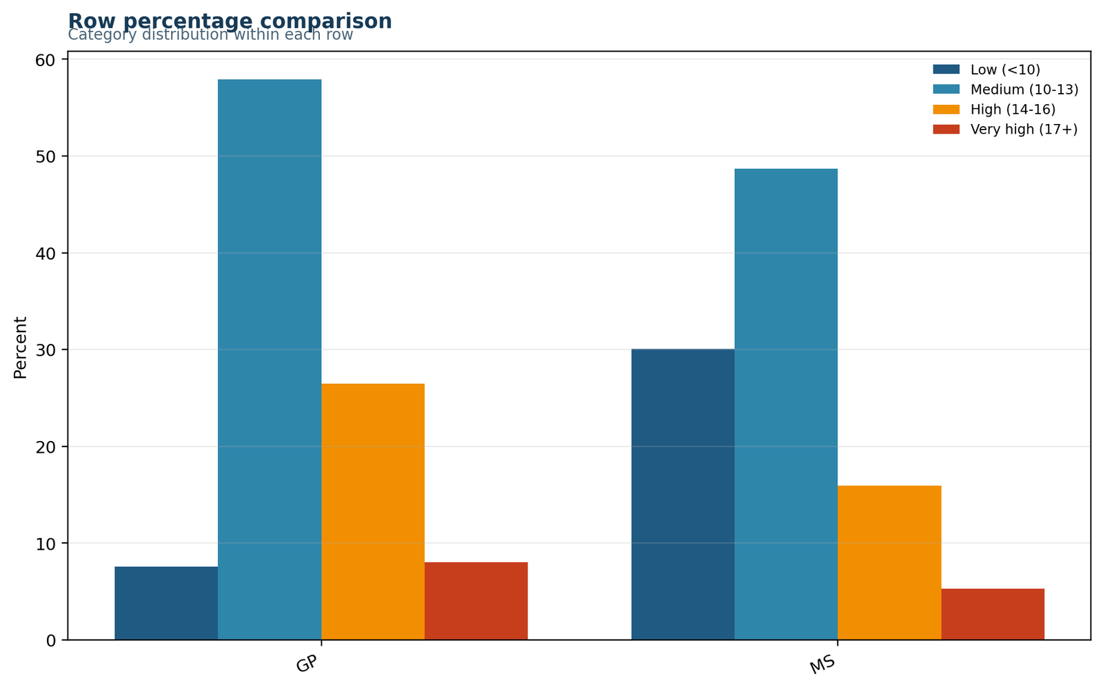
Within-GP Percentages
- Low: 7.57%
- Medium: 57.92%
- High: 26.48%
- Very high: 8.04%
Within-MS Percentages
- Low: 30.09%
- Medium: 48.67%
- High: 15.93%
- Very high: 5.31%
First Descriptive Reading
The Low category contains 7.57% of GP students but 30.09% of MS students. GP has higher within-school percentages in Medium, High and Very high categories. These differences motivate the inferential test but do not replace it.
See Cross-Tabulation and Frequency Distribution for additional table-reading guidance.
Selecting a Categorical Data Analysis Method in Python
Use counts, proportions, confidence intervals and a goodness-of-fit test when comparing with prespecified probabilities.
Use a contingency table, Pearson chi-square, exact tests, Cramer's V and residual analysis.
Use a paired binary method because ordinary independence assumptions are violated.
Use a square-table symmetry or marginal-homogeneity procedure.
Use binary logistic regression for adjusted probabilities and odds ratios.
Use multinomial logistic regression when the outcome has more than two unordered categories.
Why Pearson Chi-Square Is Primary Here
The records are independent, both variables are categorical, the table is 2 × 4 and every expected count exceeds 5. These conditions make Pearson's chi-square test a suitable primary method.
Why an Exact Test Is Still Useful
An exact conditional test provides a valuable reproducibility check because it does not depend on the asymptotic chi-square approximation. In this large, well-supported table, the exact and asymptotic conclusions agree.
Why a Single Odds Ratio Is Not Used
An odds ratio naturally summarizes a 2 × 2 table. The current outcome has four categories, so forcing one odds ratio would require collapsing information. Cramer's V provides an overall association magnitude without changing the table.
Complete Categorical Data Analysis in Python Results
| Method or measure | Statistic | Degrees of freedom | P-value | Interpretation |
|---|---|---|---|---|
| Pearson chi-square | 59.534045213 | 3 | 7.392451635e-13 | Reject independence. |
| Likelihood-ratio chi-square | 57.075209233 | 3 | 2.476613204e-12 | Confirms the association. |
| Fisher–Freeman–Halton exact | Probability ordering | Conditional | 2.418553004e-12 | Exact result confirms the conclusion. |
| Cramer's V | 0.302872853 | — | — | Meaningful overall association. |
| Contingency coefficient | 0.289869376 | — | — | Alternative bounded association measure. |
Evidence
All three inferential approaches produce extremely small p-values. The school and final-grade category variables are not independent.
Magnitude
Cramer's V = 0.303. The result is not merely statistically detectable; the distributional difference is large enough to require substantive interpretation.
Adequacy
The smallest expected count is 16.02, and 0 expected cells are below 5. The Pearson approximation is well supported.
Plain-Language Interpretation
Students at GP are much less likely to fall in the Low grade band and more likely to appear in the Medium, High or Very high bands than students at MS. The largest difference occurs in the Low category, which drives more than four-fifths of the total chi-square when its two school cells are combined.
Expected Counts and Chi-Square Assumptions
| School | Low expected | Medium expected | High expected | Very high expected |
|---|---|---|---|---|
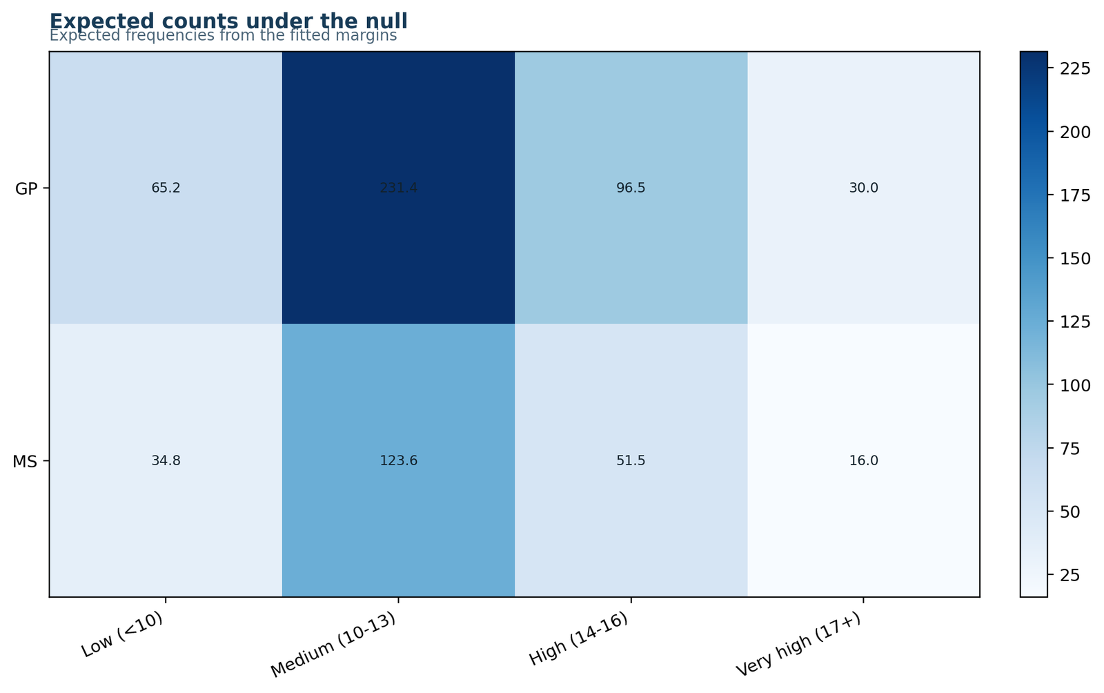
| GP | 65.177196 | 231.379045 | 96.462250 | 29.981510 |
| MS | 34.822804 | 123.620955 | 51.537750 | 16.018490 |
Minimum Expected Count
The minimum expected count is 16.018490, comfortably above 5.
Cells Below Five
0 of 8 cells have expected counts below 5.
Independence
Each student must contribute to only one cell. Expected-count adequacy does not repair dependent records.
Expected-Count Formula
For GP and Low, the expected count is 423 × 100 / 649 = 65.177. Only 32 students are observed, creating a large negative residual.
Expected Counts Are a Null-Model Benchmark
Expected counts are not predictions of individual grades. They are the counts that would occur, given the observed margins, if school and grade band were independent.
Other Important Assumptions
- Categories are mutually exclusive and collectively meaningful.
- The sampling process supports the population interpretation.
- Observations are independent.
- Missingness and category construction do not create serious bias.
- The analysis plan was not selected only after viewing the table.
Pearson Residuals, Adjusted Residuals and Cell Contributions
| Cell | Observed | Expected | Pearson residual | Adjusted residual | Chi-square contribution | Share of total |
|---|---|---|---|---|---|---|
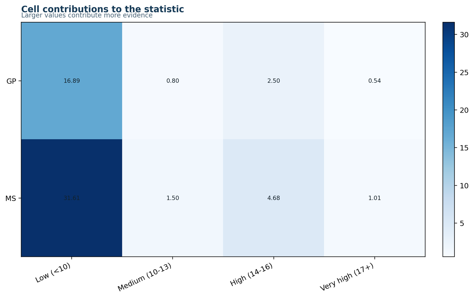
| GP × Low | 32 | 65.177 | -4.110 | -7.572 | 16.888 | 28.37% |
| GP × Medium | 245 | 231.379 | 0.895 | 2.255 | 0.802 | 1.35% |
| GP × High | 112 | 96.462 | 1.582 | 3.051 | 2.503 | 4.20% |
| GP × Very high | 34 | 29.982 | 0.734 | 1.290 | 0.539 | 0.90% |
| MS × Low | 68 | 34.823 | 5.622 | 7.572 | 31.609 | 53.09% |
| MS × Medium | 110 | 123.621 | -1.225 | -2.255 | 1.501 | 2.52% |
| MS × High | 36 | 51.538 | -2.164 | -3.051 | 4.684 | 7.87% |
| MS × Very high | 12 | 16.018 | -1.004 | -1.290 | 1.008 | 1.69% |
Dominant Low-Grade Pattern
GP × Low has a Pearson residual of -4.11, while MS × Low has 5.62. Together, the two Low cells contribute 81.46% of the total chi-square.
Secondary High-Grade Pattern
GP × High is above expectation and MS × High is below expectation. Their adjusted residual magnitudes are 3.05, indicating another important part of the association.
Residual Sign
A positive residual means the observed count exceeds the independence expectation. A negative residual means the observed count is lower than expected. Residual magnitude helps prioritize interpretation, but post-hoc cell claims should consider multiplicity.
Contribution Versus Residual
The chi-square contribution is the squared Pearson residual. It removes direction and shows how much each cell adds to the global statistic. The residual retains direction and is therefore more useful for substantive explanation.
Effect Size for Categorical Data Analysis in Python
Cramer's V
For the worked table, V = 0.302873. Because the smaller table dimension contributes one degree of freedom, V equals the square-root chi-square-to-N ratio here.
Contingency Coefficient
The contingency coefficient is 0.289869. It is bounded below 1 in finite tables, so it is less convenient for comparison across table dimensions.
Interpreting Cramer's V
Universal labels such as small, medium and large are only rough guides. The substantive importance of V = 0.303 depends on the context, category definitions and consequences of the observed distributional difference.
Why Effect Size Is Essential
With enough observations, a minor discrepancy can produce a small p-value. Cramer's V separates evidence from magnitude. Here, both the p-value and the residual pattern indicate that the result is not driven only by sample size.
Effect Size Does Not Identify Direction
Cramer's V is nonnegative. Direction and category-specific meaning come from row percentages, column percentages and residuals.
See Cramer's V, Contingency Coefficient and Effect Size for additional interpretation.
Fisher–Freeman–Halton Exact Test for the 2 × 4 Table
Why the Exact Extension Is Used
Fisher's familiar exact test is designed for 2 × 2 tables. The Fisher–Freeman–Halton extension applies the same fixed-margin logic to larger contingency tables.
Worked Exact Result
The probability-ordering exact p-value is 2.418553004e-12. It confirms the Pearson and likelihood-ratio conclusions.
Conditional Sample Space
The exact calculation fixes both row totals and all four column totals. It enumerates every feasible first-row allocation and calculates its multivariate hypergeometric probability. Tables with probability no greater than the observed table are included in the two-sided exact p-value.
Number of Feasible Tables
The verified enumeration contains 654,334 feasible 2 × 4 tables under the fixed margins. Their probabilities sum to 1.000000000000, providing a numerical validation of the enumeration.
Exact Versus Asymptotic Results
| Method | P-value | Reference | Conclusion |
|---|---|---|---|
| Pearson chi-square | 7.392451635e-13 | Asymptotic χ²(3) | Reject independence |
| Likelihood-ratio G² | 2.476613204e-12 | Asymptotic χ²(3) | Reject independence |
| Fisher–Freeman–Halton | 2.418553004e-12 | Exact fixed-margin probability | Reject independence |
Complete Categorical Data Analysis in Python Workflow
1. Import and Inspect
Read the file, inspect dimensions, data types, missing values and category labels before creating derived variables.
2. Build Frequencies
Calculate counts and percentages for school and the G3 grade band. Verify totals before testing.
3. Create Crosstab
Use pandas.crosstab and reindex rows and columns to preserve the intended order.
4. Run Tests
Use SciPy for Pearson and likelihood-ratio chi-square calculations. Add an exact method when required.
5. Calculate Diagnostics
Derive expected counts, residuals, adjusted residuals, cell contributions and Cramer's V.
6. Plot and Report
Create labelled charts and write a result that connects statistics with the observed table.
Recommended Package Imports
import math
import numpy as np
import pandas as pd
import matplotlib.pyplot as plt
from scipy import stats
Core Quality Checks
- Print the complete observed table and margins.
- Confirm expected-count adequacy.
- Keep category order fixed in tables and charts.
- Calculate an effect size.
- Identify influential cells without overstating post-hoc significance.
- Save code, tables, charts and the software version used.
Reproducible Output Structure
A practical project can save charts to a png folder, result tables to csv, a written summary to txt and a compiled analysis report to pdf. The public article should link to the report while keeping the core values visible on the page.
Visual Results and Statistical Findings
The seven Python figures are integrated into the results discussion. The first six appear in balanced two-figure rows, while the final method-comparison figure uses a full-width layout. Each figure is followed by exact values, statistical meaning and practical interpretation.
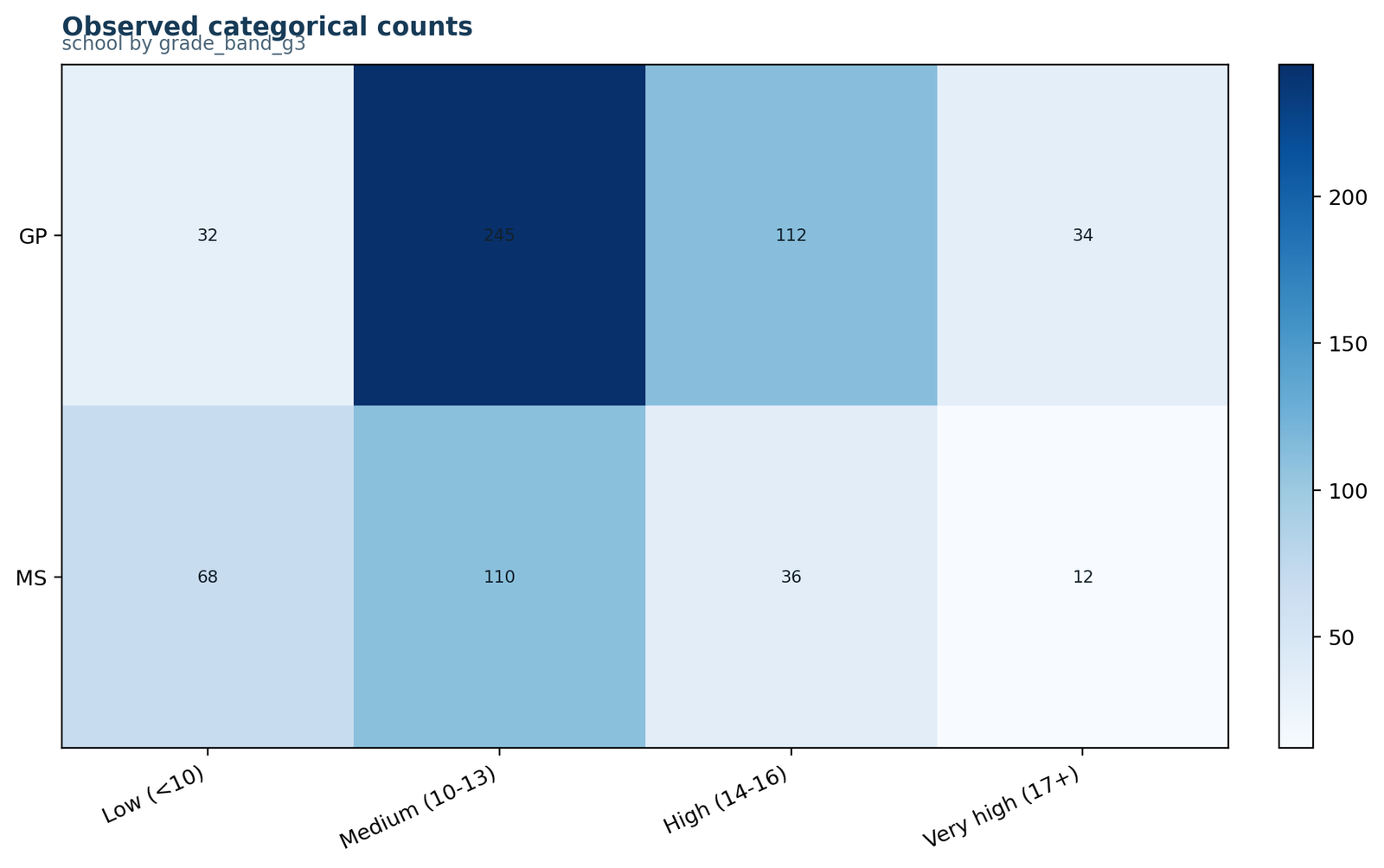
Observed School-by-Grade Frequencies
Pattern: GP contains the largest Medium and High counts, while MS has more Low cases despite its smaller total sample.
Interpretation: Raw counts reveal the table structure but must be standardized because GP has 423 students and MS has 226.
Next step: Compare observed counts with expected counts under independence.
Expected Frequencies Under Independence
Pattern: The largest expected cell is GP × Medium, while the minimum expected cell is MS × Very high.
Interpretation: Every expected count is above 5, so the asymptotic Pearson chi-square reference is appropriate.
Next step: Subtract expected counts from observed counts and standardize the differences.
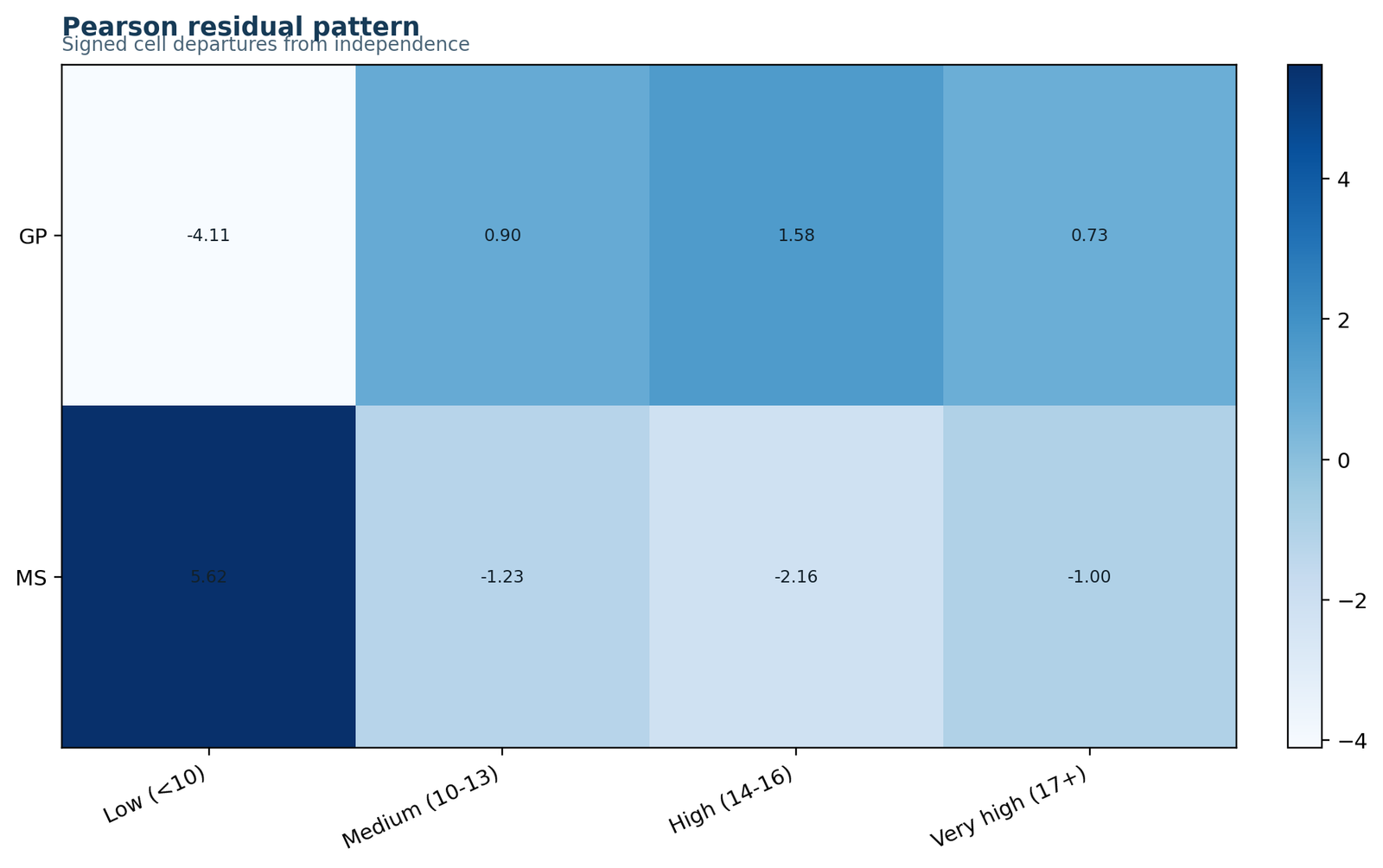
Where the Association Is Strongest
Pattern: The strongest negative residual is GP × Low, and the strongest positive residual is MS × Low.
Interpretation: The Low-grade cells provide the clearest directional evidence. GP has far fewer Low cases than expected; MS has far more.
Next step: Use adjusted residuals when evaluating cell-level extremeness.
Cells Driving the Chi-Square Result
Pattern: MS × Low contributes the most, followed by GP × Low. The remaining cells provide smaller additions.
Interpretation: The Low category accounts for most of the global association. Squared contributions show importance but not direction.
Next step: Combine contribution magnitude with residual sign.
Within-School Grade Distributions
Pattern: MS has a much larger Low percentage, while GP has larger Medium, High and Very high percentages.
Interpretation: Row percentages answer the substantive question more directly than raw counts because each school is standardized to 100%.
Next step: Report the most meaningful percentage contrasts beside the chi-square result.
Evidence, Effect Size and Assumption Check
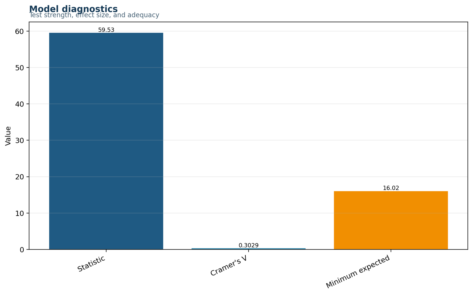
Pattern: The statistic is large, Cramer's V is about .303 and the minimum expected count is about 16.
Interpretation: The chart combines evidence, magnitude and adequacy. Strong evidence is accompanied by a meaningful association and acceptable expected counts.
Next step: Keep all three quantities in the written result.
Agreement Between Pearson and Exact Results
Pattern: Both methods produce extremely small p-values and the same inferential decision.
Interpretation: Agreement between the asymptotic and exact procedures shows that the conclusion is not sensitive to the reference method.
Next step: Report Pearson as primary and the exact result as a sensitivity confirmation.
Expandable Categorical Data Analysis in Python Code
Load the dataset and define categories
from pathlib import Path
import numpy as np
import pandas as pd

data_path = Path("dataset.csv")
df = pd.read_csv(data_path)

grade_labels = [
    "Low (<10)",
    "Medium (10-13)",
    "High (14-16)",
    "Very high (17+)",
]

df["grade_band_g3"] = pd.cut(
    pd.to_numeric(df["G3"], errors="coerce"),
    bins=[-np.inf, 9, 13, 16, np.inf],
    labels=grade_labels,
    ordered=True,
)

analysis = df[["school", "grade_band_g3"]].dropna()
Create the observed contingency table
observed = pd.crosstab(
    analysis["school"],
    analysis["grade_band_g3"],
).reindex(
    index=["GP", "MS"],
    columns=grade_labels,
    fill_value=0,
)

print(observed)
print("Row totals")
print(observed.sum(axis=1))
print("Column totals")
print(observed.sum(axis=0))
Pearson and likelihood-ratio chi-square tests
from scipy import stats

pearson = stats.chi2_contingency(
    observed.to_numpy(),
    correction=False,
)

likelihood_ratio = stats.chi2_contingency(
    observed.to_numpy(),
    correction=False,
    lambda_="log-likelihood",
)

chi2, p_value, degrees_freedom, expected = pearson
g2, g2_p, _, _ = likelihood_ratio

print(chi2, degrees_freedom, p_value)
print(g2, g2_p)
print(expected)
Cramer's V and contingency coefficient
import math

n = observed.to_numpy().sum()
rows, columns = observed.shape

cramers_v = math.sqrt(
    chi2 / (n * min(rows - 1, columns - 1))
)

contingency_coefficient = math.sqrt(
    chi2 / (chi2 + n)
)

print("Cramer's V:", cramers_v)
print("Contingency coefficient:", contingency_coefficient)
Pearson residuals and cell contributions
import numpy as np

observed_array = observed.to_numpy(dtype=float)
pearson_residuals = (
    observed_array - expected
) / np.sqrt(expected)

cell_contributions = (
    observed_array - expected
) ** 2 / expected

print(pearson_residuals)
print(cell_contributions)
print(cell_contributions.sum())
Adjusted standardized residuals
row_proportions = (
    observed_array.sum(axis=1) / n
)
column_proportions = (
    observed_array.sum(axis=0) / n
)

adjusted = np.empty_like(expected)

for i in range(rows):
    for j in range(columns):
        adjusted[i, j] = (
            observed_array[i, j] - expected[i, j]
        ) / np.sqrt(
            expected[i, j]
            * (1 - row_proportions[i])
            * (1 - column_proportions[j])
        )

print(adjusted)
Row and column percentages
row_percentages = observed.div(
    observed.sum(axis=1),
    axis=0,
) * 100

column_percentages = observed.div(
    observed.sum(axis=0),
    axis=1,
) * 100

print(row_percentages.round(2))
print(column_percentages.round(2))
Observed-count heatmap in matplotlib
import matplotlib.pyplot as plt

fig, ax = plt.subplots(figsize=(10, 5))
image = ax.imshow(observed.to_numpy(), aspect="auto")

ax.set_xticks(range(len(grade_labels)))
ax.set_xticklabels(grade_labels, rotation=20, ha="right")
ax.set_yticks(range(len(observed.index)))
ax.set_yticklabels(observed.index)

for i in range(observed.shape[0]):
    for j in range(observed.shape[1]):
        ax.text(
            j,
            i,
            int(observed.iloc[i, j]),
            ha="center",
            va="center",
        )

ax.set_title("Observed categorical counts")
fig.colorbar(image, ax=ax)
fig.tight_layout()
plt.show()
Advanced Categorical Data Analysis in Python Topics
Independence Versus Homogeneity
The numerical chi-square calculation is the same for independence and homogeneity designs, but the sampling design and wording differ. Independence usually examines two variables measured in one population; homogeneity compares a categorical distribution across separately sampled groups.
Ordered Categories and Trend Tests
Pearson chi-square ignores the order of Low, Medium, High and Very high. When a monotonic trend is the primary hypothesis, an ordinal score test or regression model can use ordering more efficiently.
Post-Hoc Residual Multiplicity
Inspecting eight cells after a significant global test creates multiple-comparison concerns. Adjusted residual thresholds or multiplicity corrections should be considered before making formal cell-specific claims.
Sparse Tables
When expected counts are small, exact conditional methods, Monte Carlo procedures or carefully justified category pooling may be preferable. The current table does not have a sparse-count problem.
Structural and Sampling Zeros
A structural zero represents an impossible combination; a sampling zero represents a possible combination not observed in the sample. The distinction changes the model and degrees of freedom.
Missing Categorical Data
Complete-case analysis is simple but can be biased when missingness is related to school or grade. Missing-category reporting, multiple imputation or model-based handling may be needed.
Survey Weights
Ordinary crosstabs treat every record equally. Complex surveys require weighted estimates and design-adjusted tests rather than unweighted Pearson chi-square.
Clustered Observations
Students within the same class or school may be correlated. Cluster-robust or multilevel models are needed when the sampling structure creates dependence.
Category Collapsing
Combining categories can improve stability but changes the research question and may hide important patterns. Cutpoints and merging rules should be chosen before examining significance.
Simpson's Paradox
A school association can change after stratifying by another variable. Additional cross-tabulations or adjusted models should be guided by causal reasoning rather than indiscriminate searching.
Log-Linear Models
Log-linear models extend contingency-table analysis to several categorical variables and interactions. They are useful when no single variable is naturally designated as the outcome.
Binary Logistic Models
When the outcome is binary and covariate adjustment is needed, logistic modelling estimates adjusted odds ratios and predicted probabilities.
Multinomial Models
A nominal multi-category outcome can be modelled directly rather than analysed only through a two-way table. This supports several predictors and category-specific effects.
Ordinal Models
An ordinal model uses the order of grade bands and can estimate cumulative probability effects, provided the model's assumptions are appropriate.
Reproducibility
A complete analysis stores category definitions, software versions, random seeds for Monte Carlo methods, generated tables, chart files and the final report.
APA Reporting for Categorical Data Analysis in Python
A complete APA-style result identifies the variables, table dimensions, sample size, chi-square statistic, degrees of freedom, p-value, effect size, assumption check and the cells responsible for the association.
Full Worked APA Result
A Pearson chi-square test of independence showed a significant association between school and final-grade category, χ²(3, N = 649) = 59.53, p < .001, Cramer's V = 0.303. All expected counts exceeded 5; the minimum expected count was 16.02. MS had more Low-grade cases than expected (68 observed, 34.82 expected), whereas GP had fewer Low-grade cases than expected (32 observed, 65.18 expected). The exact Fisher–Freeman–Halton result confirmed the association, p < .001.
Concise APA Result
School was associated with G3 grade band, χ²(3, N = 649) = 59.53, p < .001, Cramer's V = 0.303. Low grades were overrepresented at MS and underrepresented at GP.
APA-Style Methods Sentence
School and final grade were analysed in a 2 × 4 contingency table after G3 was classified as Low (<10), Medium (10–13), High (14–16), or Very high (17+); Pearson chi-square was the primary test, with Cramer's V and residual diagnostics used for interpretation.
APA Results Table
| Measure | Complete value | APA presentation |
|---|---|---|
| Sample size | 649 | N = 649 |
| Table dimensions | 2 × 4 | 2 × 4 contingency table |
| Pearson statistic | 59.534045213 | χ² = 59.53 |
| Degrees of freedom | 3 | df = 3 |
| Pearson p-value | 7.392451635e-13 | p < .001 |
| Likelihood-ratio statistic | 57.075209233 | G² = 57.08 |
| Exact p-value | 2.418553004e-12 | p < .001 |
| Cramer's V | 0.302872853 | V = 0.303 |
| Minimum expected count | 16.018489985 | minimum expected = 16.02 |
Reusable APA Templates
Significant Chi-Square Association
A r × c table compared variable 1 with variable 2, N = sample size.
The association was significant, χ²(df) = statistic, p = p-value, Cramer's V = effect size.
The largest departures involved cell descriptions, with residuals of values.
Include an assumption statement and interpret percentages, not only counts.
Nonsignificant Chi-Square Result
A chi-square test evaluated the association between variable 1 and variable 2.
The result was not significant, χ²(df, N = N) = statistic, p = p-value.
The analysis did not provide sufficient evidence of association; it did not prove that the variables were independent.
Report effect size and uncertainty even when the test is nonsignificant.
Exact Conditional Sensitivity Result
Pearson's chi-square gave χ²(df) = statistic, p = p-value.
A Fisher–Freeman–Halton exact test produced p = exact p-value.
The exact analysis confirmed/did not confirm the asymptotic conclusion.
State the exact-test definition or Monte Carlo settings when applicable.
APA Language Rules
| Avoid | Use instead | Reason |
|---|---|---|
| The variables are correlated. | The categorical variables are associated. | Correlation is not the general term for a contingency-table result. |
| p = .000 | p < .001 | The p-value is extremely small, not zero. |
| The chi-square effect was large. | Report Cramer's V and contextual interpretation. | The chi-square statistic depends on N. |
| MS caused low grades. | Low grades were overrepresented at MS. | The observational table does not establish causality. |
Common Mistakes and Final Reporting Checklist
Common Mistakes
| Mistake | Correction |
|---|---|
| Treating category codes as continuous values | Use categorical dtypes and meaningful labels. |
| Reporting raw counts without denominators | Add row or column percentages. |
| Using Pearson chi-square without expected-count checks | Print expected counts and minimum expected frequency. |
| Reporting only the p-value | Add Cramer's V, residuals and substantive percentages. |
| Interpreting every residual as a separate test | Use the global test first and address multiplicity. |
| Collapsing categories after viewing significance | Choose cutpoints from the research question. |
| Claiming causation from a cross-tabulation | Use association language and discuss confounding. |
| Ignoring missing or duplicated records | Document complete cases and verify independence. |
Public Reporting Checklist
- Define each categorical variable and category order.
- Report valid N and missing-data handling.
- Show the complete observed table.
- Report row or column percentages.
- Name the statistical test and hypotheses.
- Report χ², df and p-value.
- Check and report expected counts.
- Report Cramer's V or another suitable effect size.
- Interpret the most influential residuals.
- Include the Python package and reproducible code.
- Keep all seven Python charts inside the same post.
- Check desktop, tablet and mobile rendering before publication.
Categorical Data Analysis in Python Report and Chart Downloads
Frequently Asked Questions About Categorical Data Analysis in Python
What is categorical data analysis in Python?
It is the use of Python tools to summarize, test, visualize and model categorical variables.
Which Python libraries are most useful?
pandas, NumPy, SciPy and matplotlib cover the core frequency-table, testing, diagnostic and plotting workflow.
What is a contingency table?
It is a matrix of counts showing the joint categories of two variables.
What table is used in the worked example?
A 2 × 4 table compares GP and MS schools across four G3 grade bands.
What are the four grade bands?
Low below 10, Medium 10–13, High 14–16 and Very high 17 or above.
What is the Pearson chi-square statistic?
It is 59.534045.
What are the degrees of freedom?
There are 3 degrees of freedom.
What is the Pearson p-value?
It is 7.392451635e-13, reported as p < .001.
What is the likelihood-ratio result?
G² = 57.075209, p = 2.476613204e-12.
What is the exact p-value?
The Fisher–Freeman–Halton probability-ordering p-value is 2.418553004e-12.
What is Cramer's V?
Cramer's V is 0.302873.
What is the contingency coefficient?
It is 0.289869.
Were chi-square assumptions satisfied?
Yes. The minimum expected count is 16.02, and no expected cell is below 5.
Which cell contributes most?
MS × Low contributes 31.61, or 53.09% of the total chi-square.
What does a positive Pearson residual mean?
The observed count is higher than expected under independence.
What does a negative residual mean?
The observed count is lower than expected under independence.
Why are row percentages important?
They compare category distributions after standardizing each school to 100%.
Can a single odds ratio summarize this table?
Not without collapsing the four-category outcome, which would change the question.
When should an exact test be used?
Use an exact or Monte Carlo method when asymptotic assumptions are doubtful or as a reproducibility check.
What is Fisher–Freeman–Halton?
It is a fixed-margin exact extension of Fisher's test for larger contingency tables.
Does a significant chi-square test prove causation?
No. It identifies association, not a causal mechanism.
Can ordinal category order be used?
Yes, but Pearson chi-square itself ignores order. Ordinal models or trend tests can use it.
How should missing data be handled?
Report the rule and valid N; use a defensible missing-data method when complete-case analysis may be biased.
How do I create a crosstab in Python?
Use pandas.crosstab with explicit row and column ordering.
How do I calculate expected counts?
SciPy returns them from chi2_contingency, or calculate row total times column total divided by N.
How do I calculate Cramer's V?
Take the square root of chi-square divided by N times the smaller dimension minus one.
How do I plot the table?
Use matplotlib imshow or a labelled bar chart, and annotate exact values.
What should APA reporting include?
Variables, N, table dimensions, chi-square, df, p, Cramer's V, assumptions and influential cells.
Why is the Low category important here?
The GP and MS Low cells together account for most of the chi-square statistic.
What is the final conclusion?
School and G3 grade band are significantly associated, with a meaningful difference in the grade distributions.
Categorical Data Analysis in Python Conclusion
Statistical Conclusion
The school-by-grade-band table produced χ²(3) = 59.534045, p = 7.392e-13. The likelihood-ratio and exact conditional analyses confirmed the same conclusion.
Substantive Conclusion
GP has fewer Low-grade students and larger Medium, High and Very high percentages than MS. Cramer's V = 0.303 shows that the association deserves practical interpretation.
A strong categorical data analysis in Python does more than run one test. It defines categories transparently, shows the observed table, validates expected counts, reports an effect size, explains residuals, compares exact and asymptotic evidence, supplies reproducible code and presents charts that connect the statistics with the data pattern.

