
Ordinal Logistic Regression: Formula, Interpretation, SPSS, Python, R and Excel Guide
Ordinal Logistic Regression models an outcome whose categories have a meaningful order but whose distances are not assumed to be equal. This guide first explains the statistical method itself, then applies it to Low, Medium and High G3 achievement categories.
Cumulative logit
Accuracy 90.76%
G2 OR 6.2226
Model Overview
Ordinal Logistic Regression is a regression method for dependent variables made of ordered categories. Examples include poor/fair/good/excellent ratings, low/medium/high risk, strongly disagree through strongly agree responses, disease stages, educational achievement bands, and ranked severity levels. The categories have a natural progression, but the numerical distance between adjacent levels is not assumed to be equal. That combination—ordered categories without guaranteed equal spacing—is the reason Ordinal Logistic Regression exists.
The main purpose of Ordinal Logistic Regression is to estimate how predictor variables change the likelihood of occupying a higher rather than a lower position on an ordered outcome. Instead of modeling a continuous mean, the method models cumulative probabilities such as the probability of being above Low and the probability of being above Medium. It then combines those cumulative comparisons through a link function, most commonly the cumulative logit. This allows all outcome categories to contribute to one coherent ordered model.
Ordinal Logistic Regression is used when three conditions are met. First, the dependent variable has at least three categories. Second, those categories can be ranked meaningfully. Third, treating the categories as equally spaced numerical scores would be scientifically questionable. For example, the difference between Low and Medium achievement may not be the same as the difference between Medium and High achievement. Ordinary linear regression would impose an equal-distance interpretation, while multinomial logistic regression would ignore the known order. Ordinal Logistic Regression occupies the useful middle ground.
Why use Ordinal Logistic Regression instead of separate binary models? Separate binary models would analyze different cut-points independently and could produce inconsistent conclusions. The ordinal model uses the common ordering efficiently and estimates one set of predictor slopes across cumulative thresholds when the proportional-odds assumption is reasonable. This usually gives a more parsimonious and interpretable analysis than fitting multiple unrelated logits.
Conceptually, Ordinal Logistic Regression compares cumulative groups. With Low, Medium and High outcomes, one cumulative comparison separates Low from Medium-or-High, and a second separates Low-or-Medium from High. Under the proportional-odds model, a predictor has the same slope across both cumulative comparisons. The thresholds differ, but the predictor effect remains constant. This is the central assumption that lets one odds ratio summarize movement toward higher categories.
The coefficients from Ordinal Logistic Regression are cumulative log-odds effects. Exponentiating a coefficient gives an odds ratio for being in a higher ordered category. An odds ratio above 1 means the predictor shifts the outcome upward; an odds ratio below 1 means it shifts the outcome downward. For example, an odds ratio of 6.22 means the cumulative odds of occupying a higher category are multiplied by about 6.22 for each one-unit increase in the predictor, holding the remaining predictors constant. The odds ratio does not mean that the category itself increases by 6.22 units.
Ordinal Logistic Regression differs from Binary Logistic Regression because a binary model has only two outcome categories and one logit. It differs from multinomial logistic regression because multinomial regression treats categories as nominal and estimates separate class contrasts without using their order. It differs from ordinary linear regression because it does not assume equal intervals, normal residuals, or unconstrained continuous predictions. It belongs to the broader Generalized Linear Model family.
The method supports continuous, ordinal, binary, and categorical predictors. Numeric predictors such as age or grades enter as slopes, while categorical predictors are represented through dummy or effect coding. Interactions and nonlinear terms can also be added when theory requires them. When observations are clustered, extensions such as Generalized Estimating Equations or Hierarchical Linear Model may be more appropriate than an ordinary independent-observation model.
The key assumptions include a correctly ordered outcome, independent observations, appropriate predictor coding, absence of perfect separation, tolerable multicollinearity, and a reasonable proportional-odds or parallel-lines assumption. The proportional-odds assumption means that a predictor’s effect is stable across cumulative cut-points. If that assumption fails substantially, a partial proportional-odds model, generalized ordered logit, multinomial model, or category-specific alternative may be needed.
The advantages of Ordinal Logistic Regression are efficient use of ordering, compact effect estimates, nonnegative category probabilities that sum to 1, and interpretable cumulative odds ratios. Its limitations include sensitivity to outcome coding, difficulty explaining thresholds, reliance on the proportional-odds assumption, and the possibility that predicted hard categories conceal uncertainty. Therefore, probabilities, confusion patterns, and class-specific performance should be reported along with coefficients.
Only after establishing that foundation should the current worked scenario be introduced. Here, G3 is converted into Low = G3 < 10, Medium = 10 ≤ G3 < 15, and High = G3 ≥ 15. The model uses G1, G2, studytime, failures, absences, age, school, sex, and address. The fitted Ordinal Logistic Regression model has a cumulative-logit link, log likelihood -158.5859, McFadden pseudo R² 0.7268, and classification accuracy 90.76%.
The worked results show that earlier academic performance is the central process. G2 is the strongest predictor, G1 adds further information, age has a smaller positive adjusted association, and school_MS has a negative adjusted association. The model’s errors occur only between neighbouring classes, which indicates that the ordering is captured well even when the exact category is missed.
Quick Answer
Outcome coding
- Low: G3 < 10
- Medium: 10 ≤ G3 < 15
- High: G3 ≥ 15
Main result
- G2 strongly moves students toward higher categories.
- G1 and age also increase cumulative odds.
- MS school membership reduces adjusted cumulative odds.
Table of Contents
- Why Ordinal Logistic Regression is used
- How the cumulative-logit model works
- Variables used and coding
- Results at a glance
- Eight Python chart stories
- R chart interpretation
- Complete coefficient results
- Probability and prediction interpretation
- Assumptions and diagnostics
- SPSS, Python, R and Excel
- Code
- Advanced interpretation
- APA-style reporting
- Publication checklist
- Downloads
- Related Salar Cafe guides
- Frequently asked questions
Why Ordinal Logistic Regression Is Used
Ordinal Logistic Regression is used because the category order contains information that should not be discarded. A multinomial model would treat Low, Medium and High as unrelated labels, while linear regression would treat 1, 2 and 3 as equally spaced measurements. The cumulative-logit model uses the ordering without imposing equal distances.
The method also answers a more useful substantive question than a sequence of binary models: how do predictors shift the overall likelihood of occupying a higher category? This is especially appropriate for ratings, severity levels, achievement bands and response scales.
The current outcome has enough cases in every category—100 Low, 418 Medium and 131 High—to estimate two cumulative thresholds. The model therefore uses the complete ordered information rather than reducing the outcome to pass/fail.
How the Cumulative-Logit Model Works
Low < Medium < High.
Low versus higher and Low-or-Medium versus High.
Category probabilities sum to 1 for each case.
The thresholds define where the cumulative response changes category. The fitted transformed cumulative-logit thresholds are approximately 27.8623 for Low/Medium and 40.6053 for Medium/High under the workbook’s reporting convention.
The proportional-odds structure uses the same predictor vector β at both thresholds. That means a predictor such as G2 has one cumulative odds ratio rather than a different coefficient for each boundary. This compact structure is the primary strength of Ordinal Logistic Regression, but it must be checked for plausibility.
In Ordinal Logistic Regression, the cumulative logits share one predictor slope under the proportional-odds assumption, while the thresholds separate adjacent outcome levels.
Variables Used and Coding
| Variable | Role | Definition | Model use |
|---|---|---|---|
| g3_ordinal | Ordered outcome | Low, Medium, High from G3 | Dependent variable |
| G1 | Numeric predictor | First-period grade | Academic predictor |
| G2 | Numeric predictor | Second-period grade | Strongest academic predictor |
| studytime | Numeric predictor | Study-time category | Adjusted predictor |
| failures | Numeric predictor | Previous failures | Adjusted predictor |
| absences | Numeric predictor | Absence count | Adjusted predictor |
| age | Numeric predictor | Age in years | Adjusted predictor |
| school_MS | Dummy predictor | MS compared with GP | Categorical contrast |
| sex_M | Dummy predictor | Male compared with female | Categorical contrast |
| address_U | Dummy predictor | Urban compared with rural | Categorical contrast |
The coding stage is central to Ordinal Logistic Regression because reversing the category order reverses the direction of every cumulative odds interpretation.
Results at a Glance
Full model
Intercept-only comparison
Model comparison
Penalty-adjusted fit
Strong improvement
589/649 correct
These results show why Ordinal Logistic Regression should be judged through model fit, ordered probabilities, and class-specific performance rather than accuracy alone.
Open the Main Output
McFadden pseudo R² should not be interpreted as ordinary variance explained. Use the Adjusted R-Squared, Effect Size and P-Value guides to distinguish model improvement, practical importance and statistical evidence. This Ordinal Logistic Regression result should therefore be interpreted as strong ordered-category discrimination rather than as ordinary explained variance.
Eight Python Chart Stories: What Each Ordinal Logistic Regression Figure Actually Means
Each figure is interpreted in four stages: the visible pattern, the exact values, the substantive meaning, and the decision-relevant conclusion. The aim is to help students, researchers, and practitioners understand both the statistical result and its practical importance.
Chart 1: Ordinal Outcome Distribution
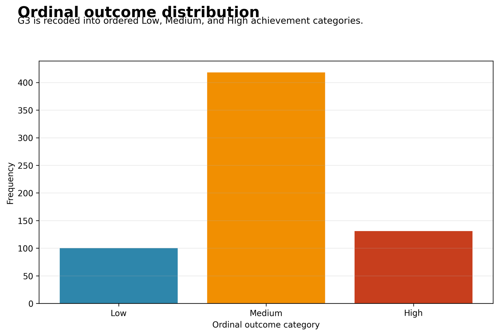
Medium contains most of the sample, with smaller Low and High groups on either side.
Low: 100 students (15.41%); Medium: 418 (64.41%); High: 131 (20.18%). Total: 649 students.
Nearly two-thirds of students fall in the Medium category. The model therefore has more information for estimating the middle band than either extreme. Low and High still contain enough observations for meaningful estimation, but performance should not be judged from overall accuracy alone because the classes are unequal in size.
The Low category contains the fewest students and is the most vulnerable to missed classifications. Class-specific recall, precision, and the confusion matrix provide a fairer assessment than the overall accuracy by itself.
Chart 2: Observed Versus Predicted Category Counts
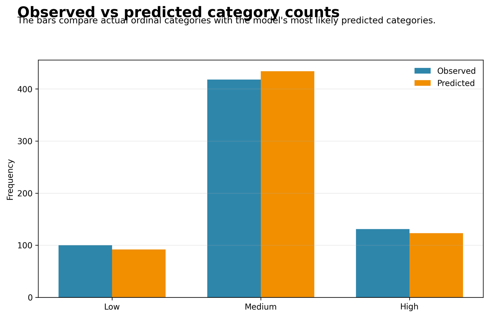
Predicted class totals remain close to the observed totals, with a small shift from both extremes into Medium.
Observed: 100 Low, 418 Medium, and 131 High. Predicted: 92 Low, 434 Medium, and 123 High. The differences are −8, +16, and −8.
The model preserves the overall outcome distribution but is slightly cautious about assigning the extreme categories. Students near the Low–Medium and Medium–High boundaries are more likely to be placed in Medium than pushed to the opposite extreme.
The predicted class mix is realistic at the population level. For screening or individual decisions, borderline cases need their full probability profile reviewed because the most likely label can hide uncertainty between adjacent categories.
Chart 3: Average Predicted Probabilities
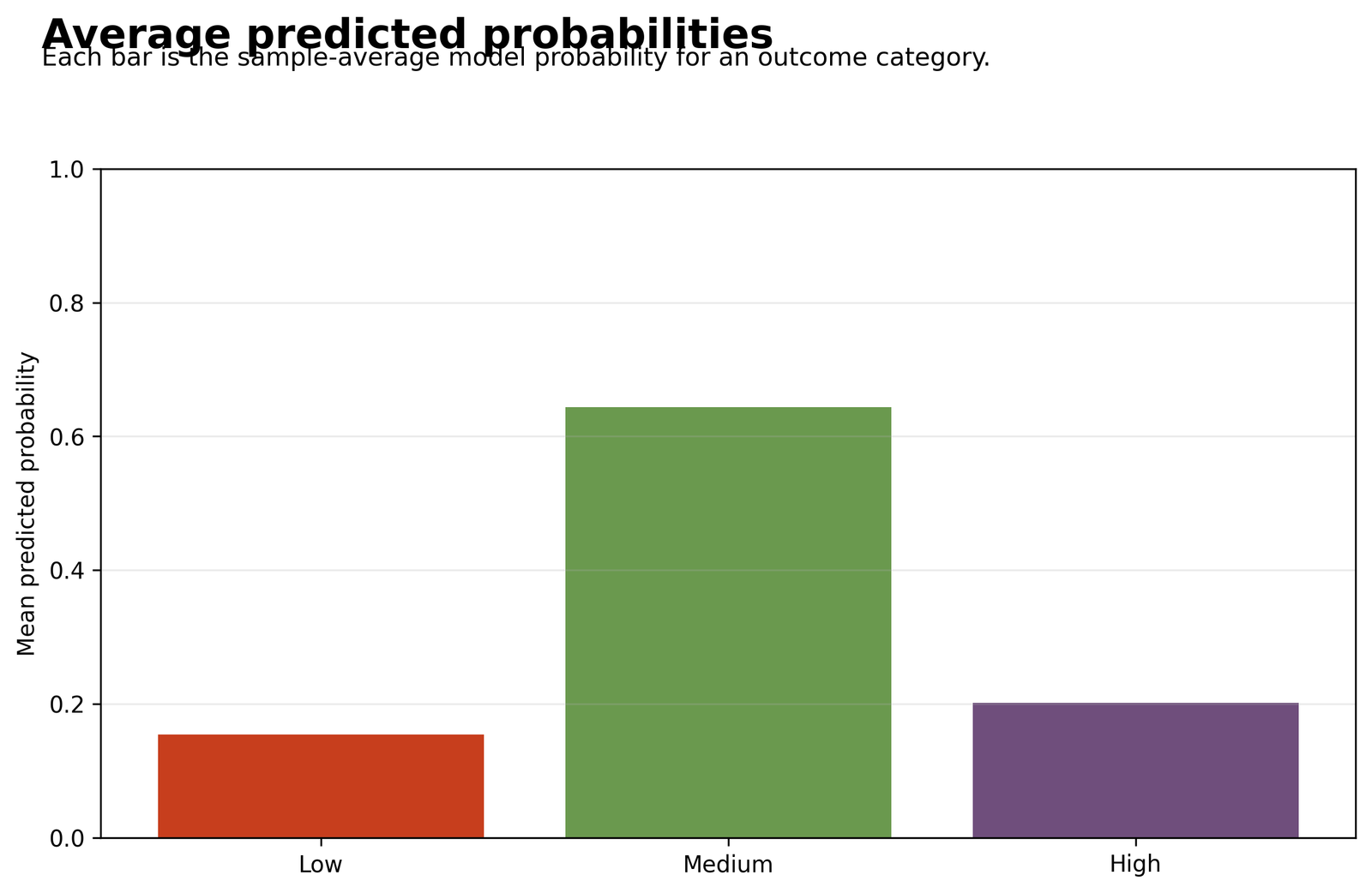
Average predicted probability is highest for Medium and much lower for Low and High.
Average probabilities are approximately 0.154 for Low, 0.644 for Medium, and 0.202 for High. These closely match the observed proportions of 15.41%, 64.41%, and 20.18%.
Across the full sample, the model allocates probability in almost the same proportions as the observed outcome. It is not overproducing High predictions or collapsing most students into Low. Medium receives the largest share because it is both the most common outcome and the main destination for uncertain boundary cases.
The close match supports class-level calibration. It does not mean every individual prediction is certain; two students assigned to Medium may have very different probability profiles.
Chart 4: Ordinal Logistic Odds Ratios
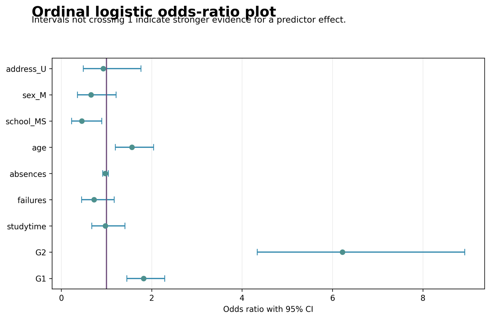
G2 has the largest positive odds ratio, followed by G1 and age, while school MS is associated with lower cumulative odds.
G2: OR = 6.223, 95% CI [4.336, 8.930]; G1: OR = 1.820, CI [1.448, 2.287]; age: OR = 1.563, CI [1.196, 2.041]; school MS: OR = 0.452, CI [0.228, 0.894]. Other intervals cross 1.
Second-period grade is the strongest independent indicator of movement into a higher final-grade category. G1 still contributes after G2 is included, but its effect is much smaller. Age has a modest positive association, while otherwise comparable MS students have lower cumulative odds of occupying a higher category than GP students.
A one-point increase in G2 multiplies the cumulative odds of being above a category threshold by about 6.22, holding the other predictors constant. Studytime, failures, absences, sex, and address do not show a separate reliable shift after the stronger predictors are accounted for.
Chart 5: Classification Table Heatmap
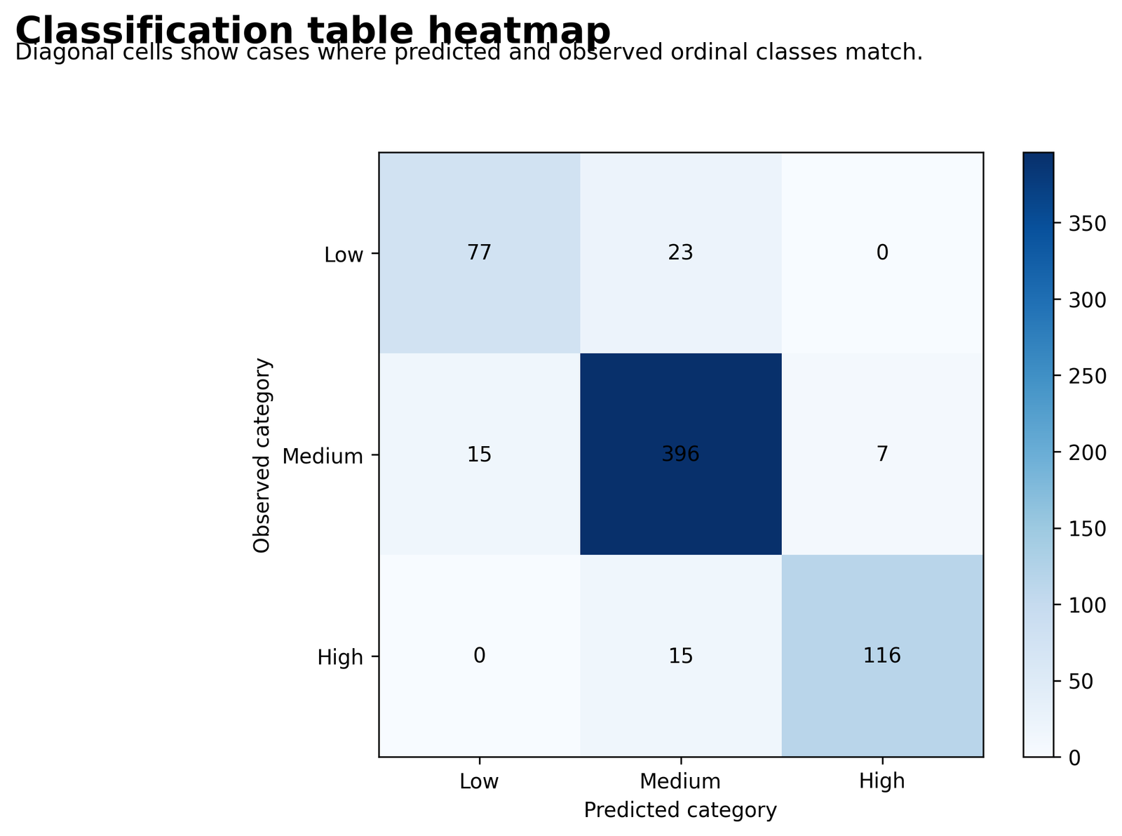
Most cases lie on the diagonal, and every error moves only one category up or down.
77 Low, 396 Medium, and 116 High are classified correctly, giving 589 correct predictions. Errors: 23 Low→Medium, 15 Medium→Low, 7 Medium→High, and 15 High→Medium. There are no Low↔High errors.
The model captures the order of the outcome well. Even when the exact category is missed, students are assigned to a neighboring category rather than the opposite extreme. The uncertain cases are concentrated around the two category boundaries.
The 90.76% accuracy is strengthened by the absence of extreme misclassification. For high-stakes use, the 23 Low students placed in Medium deserve the most attention because they may represent students whose support needs would otherwise be underestimated.
Chart 6: Ordinal Residual Distribution
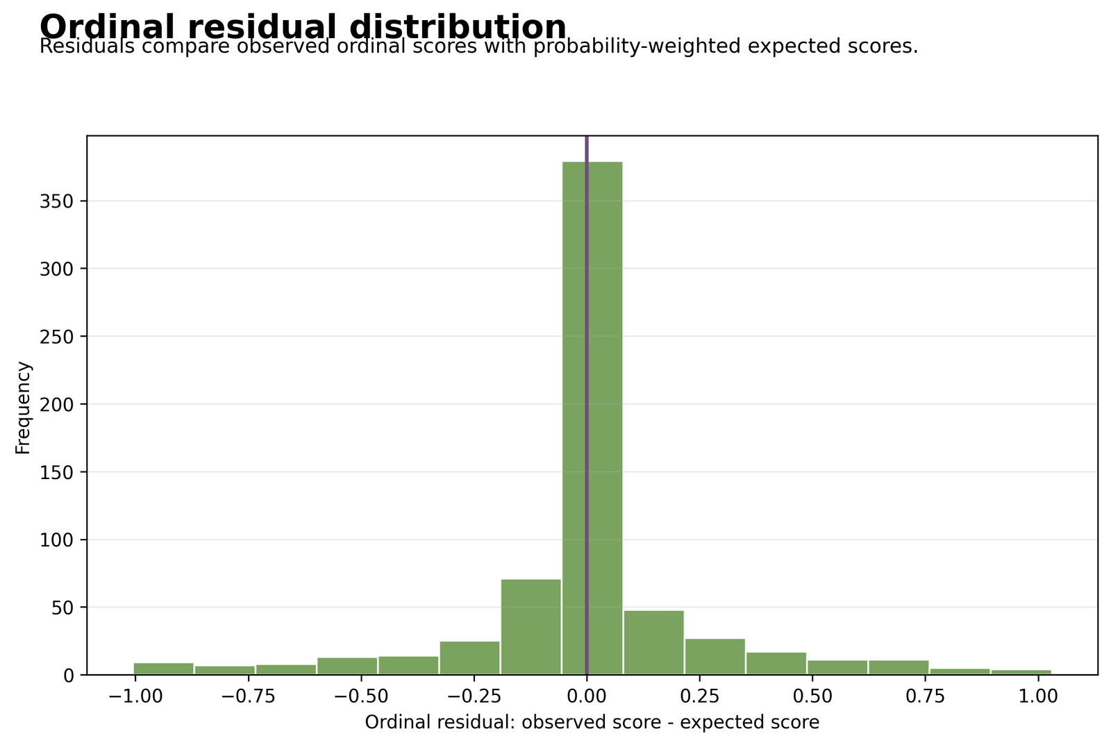
Residuals cluster near zero, with relatively few observations extending toward −1 or +1.
Ordinal scoring uses Low = 1, Medium = 2, and High = 3. Most differences between observed and probability-weighted expected scores are close to 0.
For most students, the probability-weighted expected category is close to the observed category. Larger residuals arise when the model spreads meaningful probability across neighboring categories rather than assigning a dominant probability to the observed outcome.
The tails identify students whose outcomes are not represented well by the fitted probability profile. Because the response is ordered and discrete, this distribution should be used to find unusual cases rather than judged against the normality standard used in ordinary linear regression.
Chart 7: Observed and Expected Ordinal Score by G1
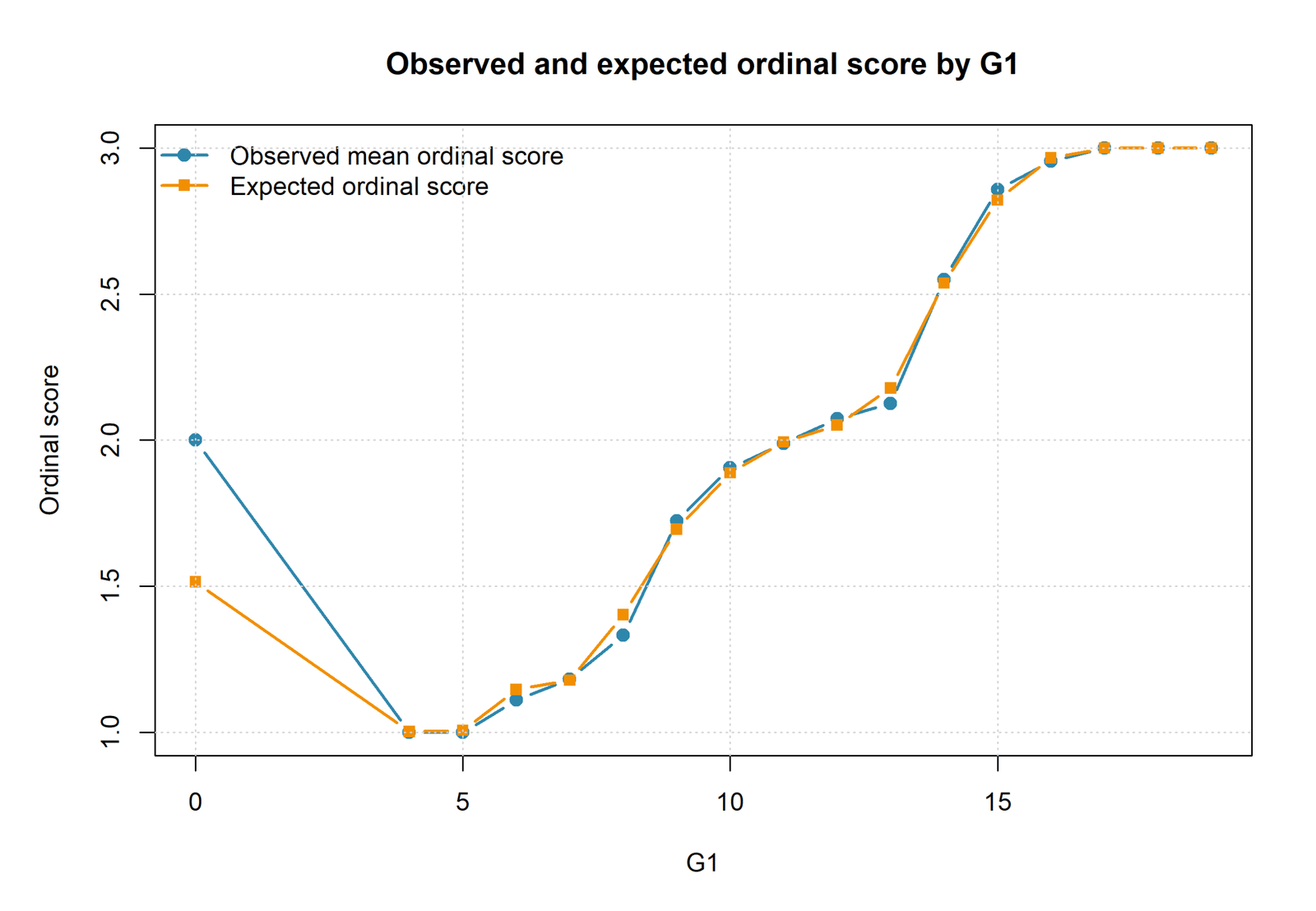
Observed and expected ordinal scores rise together as G1 increases, with close agreement across the main data range.
At G1 = 4–5, both scores are close to 1.0; near G1 = 10, both are about 1.9; near G1 = 14, they are approximately 2.54–2.56; and from G1 = 17–19, both approach 3.0.
Lower first-period grades are associated mainly with Low outcomes, middle G1 values move through Medium, and high G1 values approach High. The fitted expected score follows the observed progression closely wherever the predictor has adequate data.
G1 provides a useful early indication of the likely final category. The isolated G1 = 0 point should not drive the interpretation because a local average based on very few observations is less stable than the pattern across the populated range.
Chart 8: Predicted Category Probabilities Across G1
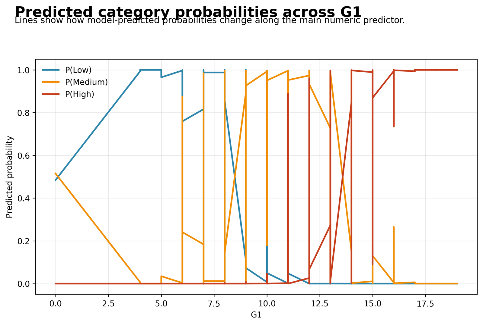
Probability moves from Low to Medium and then to High as G1 rises.
Low is most likely around G1 = 4–5. Medium dominates approximately G1 = 7–13. High becomes dominant around G1 = 15 and approaches probability 1 at the upper end. The main transition range is about G1 = 8–15.
G1 acts as an early indicator of final achievement. Students with low first-period grades are more likely to finish in Low, midrange students are most likely to finish in Medium, and students with high G1 values are increasingly likely to finish in High. Overlap in the middle is expected because G2, studytime, failures, and the other predictors also contribute to the probabilities.
The middle G1 range contains the greatest uncertainty. For students in that range, the full probability profile is more useful than a single label because it shows whether a prediction is firmly Medium or close to a Low or High boundary.
R Charts: Two Figures Followed by Two Matching Explanation Boxes
The same ordered-category visuals can be reproduced from an R cumulative-logit workflow. The explanation boxes preserve the substantive interpretation rather than merely repeating labels.
R Chart 1: Ordinal Outcome Distribution
Medium accounts for 64.41% of the sample, compared with 15.41% Low and 20.18% High. The unequal class sizes give the model more information about the middle band and make class-specific performance essential.
R Chart 2: Observed Versus Predicted Category Counts
Predicted totals remain close to the observed totals, but some Low and High cases move into Medium. The model is cautious near the two thresholds rather than confusing the opposite extremes.
R Chart 3: Average Predicted Probabilities
Average predicted probabilities closely reproduce the observed class proportions. Medium receives the largest probability share without the model artificially suppressing Low or inflating High.
R Chart 4: Ordinal Logistic Odds Ratios
G2 is the dominant predictor of upward category movement. G1 and age add smaller positive associations, while school MS is associated with lower cumulative odds. The remaining predictors do not show reliable independent shifts.
R Chart 5: Classification Table Heatmap
All 60 classification errors occur between neighboring categories. None move directly between Low and High, indicating that the model captures the ordering even when it misses the exact category.
R Chart 6: Ordinal Residual Distribution
Most probability-weighted expected scores are close to the observed ordinal scores. Larger residuals identify cases whose probability is spread across neighboring outcomes.
R Chart 7: Observed and Expected Ordinal Score by G1
Observed and expected category scores rise together across the populated G1 range. The relationship moves from Low at small G1 values, through Medium, and toward High at larger values.
R Chart 8: Predicted Category Probabilities Across G1
As G1 rises, probability shifts from Low to Medium and then to High. The middle range contains overlap because the remaining predictors also affect each student’s probability profile.
Complete Ordinal Logistic Regression Coefficient Results
| Term | B | SE | z | p | Odds ratio | 95% CI | Interpretation |
|---|---|---|---|---|---|---|---|
| G1 | 0.5988 | 0.1166 | 5.1362 | <.001 | 1.8198 | 1.4481–2.2870 | Higher G1 increases the odds of being in a higher category. |
| G2 | 1.8282 | 0.1843 | 9.9203 | <.001 | 6.2226 | 4.3361–8.9296 | G2 is the dominant predictor of movement toward higher categories. |
| studytime | -0.0253 | 0.1879 | -0.1344 | 0.8930 | 0.9751 | 0.6747–1.4092 | No independent ordered-category effect after adjustment. |
| failures | -0.3228 | 0.2448 | -1.3187 | 0.1873 | 0.7241 | 0.4482–1.1699 | Negative direction, but the interval includes 1. |
| absences | -0.0237 | 0.0327 | -0.7238 | 0.4692 | 0.9766 | 0.9159–1.0413 | No clear independent effect. |
| age | 0.4463 | 0.1363 | 3.2736 | 0.0011 | 1.5626 | 1.1962–2.0413 | Older students have higher adjusted odds of a higher category in this sample. |
| school_MS | -0.7942 | 0.3481 | -2.2818 | 0.0225 | 0.4519 | 0.2284–0.8940 | MS students have lower adjusted odds of a higher category than GP students. |
| sex_M | -0.4212 | 0.3126 | -1.3476 | 0.1778 | 0.6563 | 0.3556–1.2109 | No clear independent sex effect. |
| address_U | -0.0754 | 0.3283 | -0.2298 | 0.8183 | 0.9273 | 0.4873–1.7648 | No clear independent address effect. |
The coefficient table shows a concentrated academic pattern. G2 has the largest absolute z-value and the largest reliable odds ratio. G1 adds further positive information, while age and school_MS retain smaller adjusted associations. The remaining predictors do not have confidence intervals that exclude 1.
Probability and Prediction Interpretation
Ordinal Logistic Regression is most useful when predicted probabilities are interpreted as ordered risk profiles rather than only as hard labels.
Class-level results
- Low recall: 77.00%
- Medium recall: 94.74%
- High recall: 88.55%
Prediction precision
- Low precision: 83.70%
- Medium precision: 91.24%
- High precision: 94.31%
For every student, Ordinal Logistic Regression returns P(Low), P(Medium) and P(High). The largest probability determines the predicted category, while the probability-weighted expected score summarizes the position on the 1–3 ordinal scale. The workbook’s example profile produces P(Low) = 0.0007, P(Medium) = 0.9950, P(High) = 0.0043, an expected score of 2.0037, and a predicted category of Medium.
The probabilities are more informative than the final label. A Medium prediction with 0.99 probability is very different from a Medium prediction formed by two nearly tied probabilities. Borderline students should therefore be identified through probability profiles, not only the confusion matrix. Ordinal Logistic Regression is especially valuable here because it preserves the full probability distribution across the ordered categories.
For practical prediction, Ordinal Logistic Regression is most informative when the full probability profile is retained instead of reducing each student to a single hard category.
Assumptions, Diagnostics and Model Choice
In Ordinal Logistic Regression, diagnostics should evaluate both predictive performance and the proportional-odds structure rather than relying on accuracy alone.
Core assumptions
- Correct category order
- Independent observations
- Proportional odds or parallel lines
- Reasonable logit linearity
- No severe multicollinearity
- No dominating influential cases
Observed model behavior
- Strong model fit
- Errors only between adjacent categories
- Residuals concentrated near zero
- G1 and G2 dominate prediction
- Sparse extreme G1 values need caution
The most important assumption is proportional odds. The same slope is used for Low versus higher categories and Low-or-Medium versus High. A formal parallel-lines or Brant-type test should be reported when available. If a predictor violates the assumption strongly, a partial proportional-odds model may be more appropriate.
Check G1 and G2 using Variance Inflation Factor and Tolerance Statistic because the two grade predictors are expected to overlap. Review Cook’s Distance, Mahalanobis Distance and Influence Diagnostics for unusual cases. These checks matter even when classification accuracy is high.
Choose Ordinal Logistic Regression rather than multinomial logistic regression when the ordering is substantively meaningful and proportional odds is acceptable. Choose Binary Logistic Regression when there are only two classes, and consider Generalized Estimating Equations or Hierarchical Linear Model when observations are correlated or nested. A defensible Ordinal Logistic Regression conclusion depends on both model performance and the proportional-odds assessment.
A defensible Ordinal Logistic Regression analysis therefore combines the proportional-odds check with residual, influence, calibration, and class-performance evidence.
SPSS, Python, R and Excel Workflows
Ordinal Logistic Regression can be estimated consistently across Python, R, SPSS, and Excel-supported workflows when category coding and reference direction are documented.
Python
Python fits the cumulative-logit model, calculates category probabilities, expected scores, odds ratios and the classification table.
- Eight diagnostic charts
- Threshold and coefficient tables
- Probability-based diagnostics
R
R can fit the proportional-odds model with packages such as MASS or ordinal and can test or relax the parallel-lines assumption.
- Cumulative-logit coefficients
- Predicted probabilities
- Proportional-odds diagnostics
SPSS
SPSS uses PLUM for ordinal regression and provides thresholds, parameter estimates, model fitting information, goodness-of-fit statistics and the test of parallel lines.
- Ordered category definition
- Reference and link selection
- Parallel-lines assessment
Excel
The worked workbook contains model-fit values, coefficients, thresholds, a prediction calculator and worked probability formulas.
- Editable predictor inputs
- P(Low), P(Medium), P(High)
- Expected score and predicted class
General navigation support is available in the site’s guides for Python, R, SPSS and Excel.
Code: Expand Only the Software You Need
Python Ordinal Logistic Regression code
import pandas as pd
from statsmodels.miscmodels.ordinal_model import OrderedModel


df = pd.read_csv("dataset.csv")
df["g3_ordinal"] = pd.cut(
    df["G3"],
    bins=[-float("inf"), 9, 14, float("inf")],
    labels=["Low", "Medium", "High"],
    ordered=True
)

X = pd.get_dummies(
    df[["G1", "G2", "studytime", "failures", "absences",
        "age", "school", "sex", "address"]],
    columns=["school", "sex", "address"],
    drop_first=True,
    dtype=float
)

model = OrderedModel(df["g3_ordinal"], X, distr="logit")
result = model.fit(method="bfgs", disp=False)
probabilities = result.model.predict(result.params)
print(result.summary())
R Ordinal Logistic Regression code
library(MASS)

df <- read.csv("dataset.csv")
df$g3_ordinal <- cut(
  df$G3,
  breaks = c(-Inf, 9, 14, Inf),
  labels = c("Low", "Medium", "High"),
  ordered_result = TRUE
)

fit <- polr(
  g3_ordinal ~ G1 + G2 + studytime + failures + absences +
    age + school + sex + address,
  data = df,
  method = "logistic",
  Hess = TRUE
)
summary(fit)
exp(coef(fit))
prob <- predict(fit, type = "probs")
SPSS Ordinal Logistic Regression syntax
RECODE G3
 (Lowest thru 9=1)
 (10 thru 14=2)
 (15 thru Highest=3) INTO g3_ordinal.
VALUE LABELS g3_ordinal
 1 'Low' 2 'Medium' 3 'High'.

PLUM g3_ordinal WITH G1 G2 studytime failures absences age
 BY school sex address
 /CRITERIA=CIN(95) DELTA(0) MXITER(100) MXSTEP(5)
 /LINK=LOGIT
 /PRINT=FIT PARAMETER SUMMARY TPARALLEL.
Excel probability formulas
Linear predictor:
=SUMPRODUCT(InputValues,Coefficients)

Cumulative probability at threshold 1:
=1/(1+EXP(-(Threshold1-LinearPredictor)))

Cumulative probability at threshold 2:
=1/(1+EXP(-(Threshold2-LinearPredictor)))

P(Low):
=Cumulative1

P(Medium):
=Cumulative2-Cumulative1

P(High):
=1-Cumulative2

Expected ordinal score:
=1*P_Low+2*P_Medium+3*P_High
Advanced Interpretation and Extensions
Advanced Ordinal Logistic Regression interpretation should distinguish model fit, proportional odds, classification quality, and practical effect magnitude.
Definition of an ordinal outcome
An ordinal outcome contains categories with a meaningful rank but no guarantee that adjacent differences are equal. This is the defining reason to use Ordinal Logistic Regression.
Cumulative probabilities
The model works with cumulative probabilities such as P(Y ≤ Low) and P(Y ≤ Medium). Category probabilities are recovered by subtracting adjacent cumulative probabilities.
Cumulative logits
A cumulative logit transforms a cumulative probability into log odds. Each threshold has its own intercept or cut-point, while the proportional-odds model shares predictor slopes.
Proportional-odds assumption
The proportional-odds assumption requires a predictor to have the same cumulative slope across thresholds. It should be checked rather than assumed automatically.
Parallel-lines test
SPSS reports a test of parallel lines. A strong rejection suggests that at least one predictor effect differs across cumulative boundaries and that a generalized model may be required.
Partial proportional odds
A partial proportional-odds model permits selected predictors to vary across thresholds while retaining common slopes for predictors that satisfy the assumption.
Threshold interpretation
Thresholds locate the cumulative boundaries on the latent logit scale. They are not ordinary regression intercepts and usually receive less substantive attention than predictor effects.
Odds ratio interpretation
An odds ratio describes cumulative movement toward a higher outcome. It should be translated into probabilities for realistic profiles because odds are not identical to probability differences.
Predicted probabilities
Predicted probabilities show how a student’s risk or achievement profile is distributed across all ordered categories. They are more informative than one hard predicted class.
Expected ordinal score
A probability-weighted score summarizes the predicted position on the ordinal scale. It is useful diagnostically but does not transform the categories into a truly continuous outcome.
Class imbalance
Medium contains 418 of 649 students. That imbalance makes overall accuracy less informative unless class-specific recall, precision and confusion directions are also reported.
Adjacent-category errors
All observed errors in this model move only one category. This indicates that the ranking is preserved even when the exact class is missed.
Ordinal versus multinomial models
Ordinal Logistic Regression uses order and usually fewer parameters. Multinomial logistic regression is safer when the categories are nominal or proportional odds is untenable.
Ordinal versus binary models
Binary Logistic Regression discards intermediate categories when an ordered outcome has more than two levels. Ordinal Logistic Regression preserves the full ranking.
Ordinal versus linear regression
Linear regression assumes equal spacing and a continuous response. Ordinal Logistic Regression avoids both assumptions and keeps predictions within valid category probabilities.
Continuous predictors
Continuous predictors enter through cumulative logit slopes. Their relationship with the logit should be approximately linear unless splines or transformed terms are added.
Categorical predictors
Categorical predictors require explicit reference coding. The sign of a dummy coefficient depends on both the reference group and the outcome ordering.
Interactions
Interactions can test whether an ordered-category effect changes across another predictor. They complicate proportional-odds interpretation and should be probed with predicted probabilities.
Multicollinearity
Use Variance Inflation Factor and Tolerance Statistic to assess overlapping predictors, especially G1 and G2.
Influential cases
Review Cook’s Distance, Mahalanobis Distance and Influence Diagnostics for cases that disproportionately change coefficients or thresholds.
Separation
Perfect or quasi-complete separation occurs when predictors almost completely determine categories. It can produce unstable, extremely large estimates and convergence problems.
Sample size
Sample adequacy depends on the smallest category and the number of predictors. Use Statistical Power planning rather than relying only on total n.
Pseudo R-squared
McFadden pseudo R² compares full and null log likelihoods. It is not ordinary variance explained and should not be interpreted as a percentage of outcome variance.
Classification accuracy
Accuracy evaluates the most likely class, not probability calibration or proportional odds. It must be accompanied by a confusion matrix and class-specific metrics.
Causal interpretation
Ordinal Logistic Regression estimates adjusted associations. Causal claims require temporal ordering, design-based identification and strong no-confounding assumptions.
Replication and validation
Validate thresholds, predictor effects, proportional odds and probability calibration in another cohort before using the model for consequential decisions.
APA-Style Reporting
A strong Ordinal Logistic Regression report explains both cumulative odds and predicted category probabilities in plain language.
A complete Ordinal Logistic Regression report should state the category order, reference direction, link function, thresholds, odds ratios, confidence intervals, and predictive performance.
G2 was the strongest positive predictor, B = 1.828, SE = 0.184, z = 9.920, p < .001, OR = 6.223, 95% CI [4.336, 8.930]. G1 was also positive, OR = 1.820, 95% CI [1.448, 2.287], p < .001. Age was positive, OR = 1.563, p = .001, while school_MS was negative, OR = 0.452, p = .023. Studytime, failures, absences, sex and address were not statistically significant after adjustment.
The classification table contained 77 correct Low, 396 correct Medium and 116 correct High predictions, with no Low-to-High or High-to-Low errors. Report the proportional-odds assessment, exact p-values and confidence intervals when available.
Publication Checklist and Common Mistakes
For Ordinal Logistic Regression, the reporting checklist should protect readers from ambiguous category direction and incomplete assumption reporting.
Include in the report
- Definition and order of outcome categories
- Cumulative-logit link
- Predictor coding and reference groups
- Proportional-odds assessment
- Odds ratios and confidence intervals
- Fit statistics and pseudo R²
- Predicted probabilities and confusion matrix
- Plain-language explanation of the data process
Avoid these mistakes
- Treating ordinal categories as equally spaced
- Ignoring category order
- Reporting accuracy without class counts
- Interpreting thresholds as ordinary predictors
- Ignoring proportional odds
- Calling odds ratios probability differences
- Claiming causality from regression alone
Use the guides on Null and Alternative Hypothesis, Type I and Type II Error, Effect Size and Statistical Power to strengthen planning and reporting. The final Ordinal Logistic Regression report should connect every coefficient and chart to the actual ordered movement occurring in the data.
Downloads
Frequently Asked Questions
What is Ordinal Logistic Regression?
When should Ordinal Logistic Regression be used?
What outcome is used in this example?
This point is central to the correct interpretation of Ordinal Logistic Regression.
What link function is used?
This point is central to the correct interpretation of Ordinal Logistic Regression.
What is the proportional-odds assumption?
This point is central to the correct interpretation of Ordinal Logistic Regression.
How many students were analyzed?
What was the classification accuracy?
This point is central to the correct interpretation of Ordinal Logistic Regression.
Which predictor was strongest?
This point is central to the correct interpretation of Ordinal Logistic Regression.
How is the G2 odds ratio interpreted?
This point is central to the correct interpretation of Ordinal Logistic Regression.
Was G1 significant?
This point is central to the correct interpretation of Ordinal Logistic Regression.
Which other predictors were significant?
This point is central to the correct interpretation of Ordinal Logistic Regression.
Were studytime and failures significant?
This point is central to the correct interpretation of Ordinal Logistic Regression.
What is the difference from multinomial logistic regression?
Why report probabilities?
This point is central to the correct interpretation of Ordinal Logistic Regression.
Can Ordinal Logistic Regression prove causation?
This point is central to the correct interpretation of Ordinal Logistic Regression.
How should Ordinal Logistic Regression be reported?
This point is central to the correct interpretation of Ordinal Logistic Regression.
Final Ordinal Logistic Regression Conclusion
The fitted Ordinal Logistic Regression model captures the ordered Low-to-Medium-to-High achievement process very well. It classifies 589 of 649 students correctly, and every misclassification moves only one category rather than confusing the two extremes.
The substantive result is dominated by earlier academic performance. G2 multiplies the cumulative odds of occupying a higher category by about 6.22 per one-unit increase, G1 also contributes positively, age has a smaller positive adjusted association, and MS school membership has a negative adjusted association. The remaining predictors do not add clear independent evidence after adjustment.
The charts show what those numbers mean in practice: Low dominates at weak prior grades, Medium dominates through the central range, and High becomes overwhelmingly likely at stronger prior grades. The model is therefore not merely assigning labels; it is representing an ordered transition in achievement probabilities.

