
ANOVA F Test, Group Means, p-value, Eta Squared and Assumption Diagnostics
One Way ANOVA: Formula, Interpretation, SPSS, Python, R and Excel Guide
One Way ANOVA tests whether three or more independent groups have equal means on one numeric outcome. In this worked example, G3 final grade is compared across four studytime groups. The output shows a statistically significant ANOVA result, a medium practical effect size by eta squared, and a clear group mean pattern where higher studytime groups have higher average G3 scores.
Quick Answer: One Way ANOVA Result
The worked One Way ANOVA compared mean G3 final grade across four studytime groups. The ANOVA result was F(3, 645) = 15.876, with p = 5.706e-10. Because the p-value is far below alpha = .05, the equal-means null hypothesis is rejected.
The group summary table shows mean G3 values of 10.84, 12.09, 13.23 and 13.06 for studytime groups 1 through 4. The effect size was eta squared = 0.069, meaning studytime explains about 6.9% of the observed G3 variance in this one-way ANOVA model.
Final interpretation: Studytime groups differ significantly in mean G3 final grade. Group 1 has the lowest mean, group 2 is higher, and groups 3 and 4 have the highest means. The p-value confirms a statistically significant difference, and eta squared shows that the studytime factor explains a meaningful but not dominant part of G3 variation.
Important reporting point: One Way ANOVA tells whether at least one group mean differs, but it does not by itself identify every pairwise difference. After a significant ANOVA, post hoc tests such as Tukey HSD can be used when pairwise group comparisons are required.
Table of Contents
- What Is One Way ANOVA?
- One Way ANOVA Formula
- One Way ANOVA Hypotheses
- Dataset and ANOVA Variables Used
- SPSS Output Interpretation for One Way ANOVA
- Python Chart-by-Chart Interpretation
- R Chart-by-Chart Validation
- SPSS, R, Python and Excel Workflows
- Code Blocks for One Way ANOVA
- APA Reporting Wording
- Common Mistakes
- When to Use One Way ANOVA
- Downloads and Resources
- Related Guides
- FAQs
What Is One Way ANOVA?
One Way ANOVA, or one-way analysis of variance, is used when one categorical factor has three or more independent groups and the outcome is numeric. It tests whether the group means are equal or whether at least one group mean is different.
In this example, the outcome is G3 final grade. The factor is studytime, which has four groups. The analysis compares mean G3 across those four studytime groups.
The output shows that the ANOVA is statistically significant. The group means move from 10.84 in group 1 to 13.23 in group 3, with group 4 remaining high at 13.06. This group pattern explains why the F statistic is large and the p-value is extremely small.
Simple definition: One Way ANOVA checks whether one grouping variable explains differences in a numeric outcome. In this example, it checks whether studytime group explains differences in G3 final grade.
One Way ANOVA is part of the wider ANOVA family. It connects naturally with F Distribution, Eta Squared, Cohen’s F Formula, ANOVA Effect Size, ANOVA Assumptions, ANOVA in SPSS, ANOVA in Python, and ANOVA in R.
One Way ANOVA Formula
The main One Way ANOVA idea is to compare variation between group means with variation inside groups. If between-group variation is large compared with within-group variation, the F statistic becomes large.
For this worked output, the between-group mean square is 155.026, and the within-group mean square is 9.765. Dividing those values gives the observed F statistic of about 15.876.
Model Form
The model tests whether the mean of G3 differs across studytime groups. The error term represents the variation in G3 that remains within the studytime groups.
Eta Squared Formula
The output reports eta squared = 0.069. This means the studytime factor explains about 6.9% of the observed variance in G3. For adjusted effect-size interpretation, compare this with Eta Squared, Cohen’s F Formula, and ANOVA Effect Size.
| ANOVA Component | Value | Meaning | Interpretation |
|---|---|---|---|
| SS between | 465.078 | Variation explained by studytime groups. | Group means are separated. |
| SS within | 6298.189 | Variation remaining inside groups. | Most variation still remains within groups. |
| SS total | 6763.267 | Total G3 variation. | Used for effect-size calculation. |
| MS between | 155.026 | Between-group mean square. | Numerator of the F statistic. |
| MS within | 9.765 | Error mean square. | Denominator of the F statistic. |
| F statistic | 15.876 | Ratio of between to within variation. | Large enough to reject equal means. |
One Way ANOVA Hypotheses
One Way ANOVA tests a single equal-means null hypothesis. It does not test only one pair of groups. It tests whether all group means are equal at the same time.
| Statement | Statistical Rule | Meaning |
|---|---|---|
| Null hypothesis | H0: μ1 = μ2 = μ3 = μ4 | All studytime groups have equal mean G3. |
| Alternative hypothesis | H1: At least one group mean differs | At least one studytime group has a different mean G3. |
| Decision rule | Reject H0 when p < .05 | The observed p-value is far below .05. |
Decision for this example: Reject the equal-means null hypothesis. The result F(3, 645) = 15.876, p = 5.706e-10, shows that mean G3 differs across studytime groups.
Dataset and ANOVA Variables Used
The worked example uses student performance data. The dependent variable is G3 final grade. The factor is studytime, which has four independent groups. Each group contains students with a specific studytime category.
| Studytime Group | n | Mean G3 | SD | 95% CI Low | 95% CI High | Interpretation |
|---|---|---|---|---|---|---|
| Group 1 | 212 | 10.84 | 3.22 | 10.41 | 11.28 | Lowest mean group. |
| Group 2 | 305 | 12.09 | 3.24 | 11.73 | 12.46 | Higher than group 1. |
| Group 3 | 97 | 13.23 | 2.50 | 12.73 | 13.72 | Highest mean group. |
| Group 4 | 35 | 13.06 | 3.04 | 12.05 | 14.06 | High mean with wider interval. |
The table shows both the mean pattern and the precision of each group estimate. Group 2 has the largest sample size, while group 4 has the smallest sample size and the widest confidence interval. This matters because smaller groups usually produce less precise mean estimates.
Before interpreting One Way ANOVA, it is useful to review Descriptive Statistics, Mean Median and Mode, Standard Deviation, Standard Error, Confidence Interval, P Value, and Null and Alternative Hypothesis.
SPSS Output Interpretation for One Way ANOVA
The SPSS output confirms the same One Way ANOVA result. It compares G3 across the four studytime groups, reports a significant F statistic, and supports rejection of the equal-means null hypothesis.
SPSS ANOVA Model Summary
| SPSS Output Item | Value | Interpretation |
|---|---|---|
| Dependent variable | G3 | The outcome being compared across groups. |
| Factor | studytime | The categorical grouping variable. |
| Between-groups df | 3 | Four groups produce three between-groups degrees of freedom. |
| Within-groups df | 645 | Residual degrees of freedom. |
| F statistic | 15.876 | Between-group variation is much larger than expected relative to within-group variation. |
| p-value | 5.706e-10 | The equal-means null hypothesis is rejected. |
| Eta squared | 0.069 | Studytime explains about 6.9% of G3 variance. |
SPSS Group Descriptives
| Group | n | Mean | SD | 95% CI | Meaning |
|---|---|---|---|---|---|
| 1 | 212 | 10.84 | 3.22 | 10.41 to 11.28 | Lowest average final grade. |
| 2 | 305 | 12.09 | 3.24 | 11.73 to 12.46 | Clearly above group 1. |
| 3 | 97 | 13.23 | 2.50 | 12.73 to 13.72 | Highest average final grade. |
| 4 | 35 | 13.06 | 3.04 | 12.05 to 14.06 | High mean but less precise because the group is small. |
SPSS Assumption Context
The variance check reports a median-based Levene-style p-value of 0.3804. This is above .05, so the output does not show a serious homogeneity-of-variance problem. The residual Q-Q plot still shows lower-tail departure, so normality should be described as approximate rather than perfect.
SPSS interpretation summary: The One Way ANOVA result is statistically significant, F(3, 645) = 15.876, p = 5.706e-10. The studytime group means are not equal. Group 1 is lowest, groups 3 and 4 are highest, and eta squared = 0.069 indicates a meaningful but not dominant effect size.
Python Chart-by-Chart Interpretation
The Python charts show the complete One Way ANOVA workflow: group means, distributions, observed F distribution, p-value decision, residual diagnostics, variance check and summary table.
Python Chart 1: Group Mean G3 with 95% Confidence Intervals
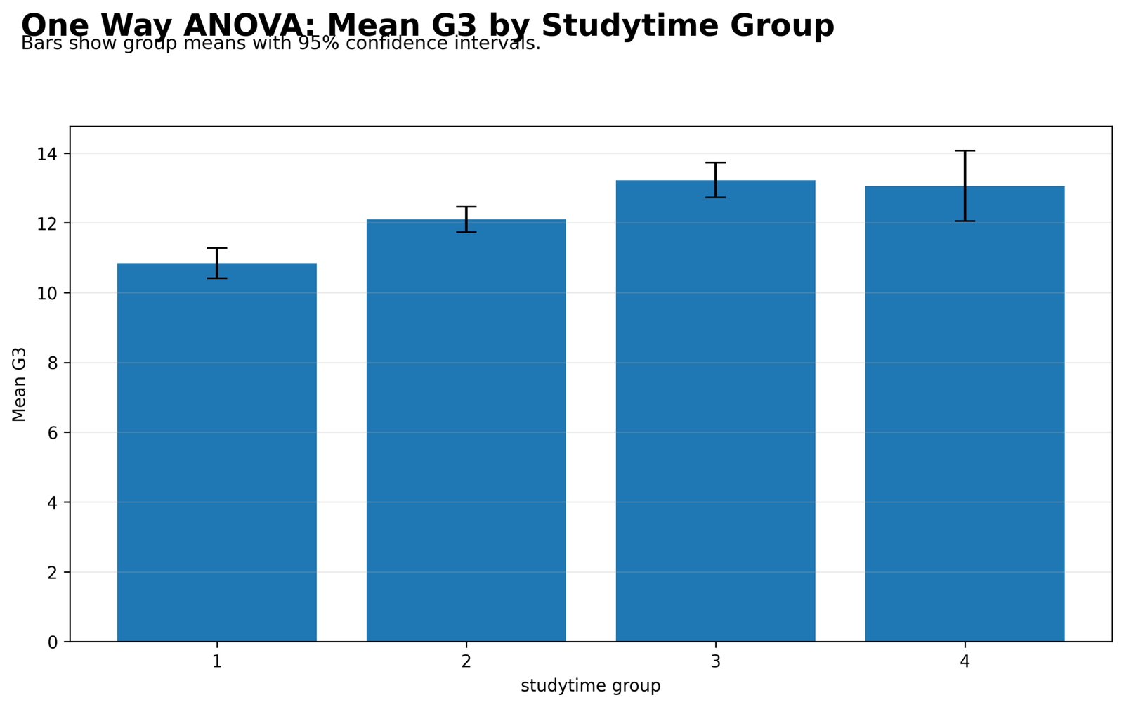
This chart shows that mean G3 rises from studytime group 1 to group 3. Group 1 has the lowest mean at about 10.84, group 2 is higher at about 12.09, group 3 is highest at about 13.23, and group 4 remains high at about 13.06.
The confidence interval for group 4 is wider than the other groups because group 4 has the smallest sample size. The mean pattern still supports the ANOVA result because the lower group and the higher groups are clearly separated.
Python Chart 2: Distribution by Studytime Group
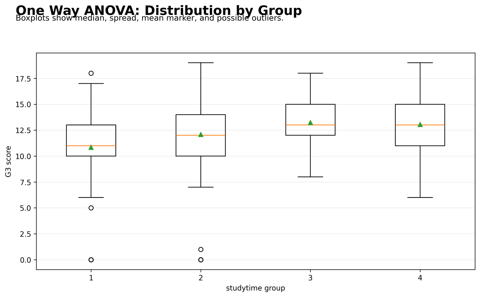
The boxplots show that groups 3 and 4 are centered higher than groups 1 and 2. Group 1 has the lowest center, while group 2 sits between the lowest and highest groups.
Low values are visible in the lower groups, including values near zero. These values explain why the residual diagnostics later show lower-tail departure. The group distributions overlap, but their centers are different enough to support a significant ANOVA.
Python Chart 3: Observed F Distribution
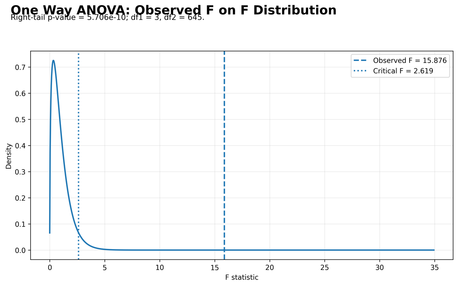
The F distribution chart shows the formal ANOVA test. The observed F statistic is 15.876 with df1 = 3 and df2 = 645. The observed F line is far to the right of the main F distribution area.
This position means the observed group mean separation is much larger than expected if all four studytime groups had the same true mean. The chart supports rejecting the equal-means null hypothesis.
Python Chart 4: p-value Decision
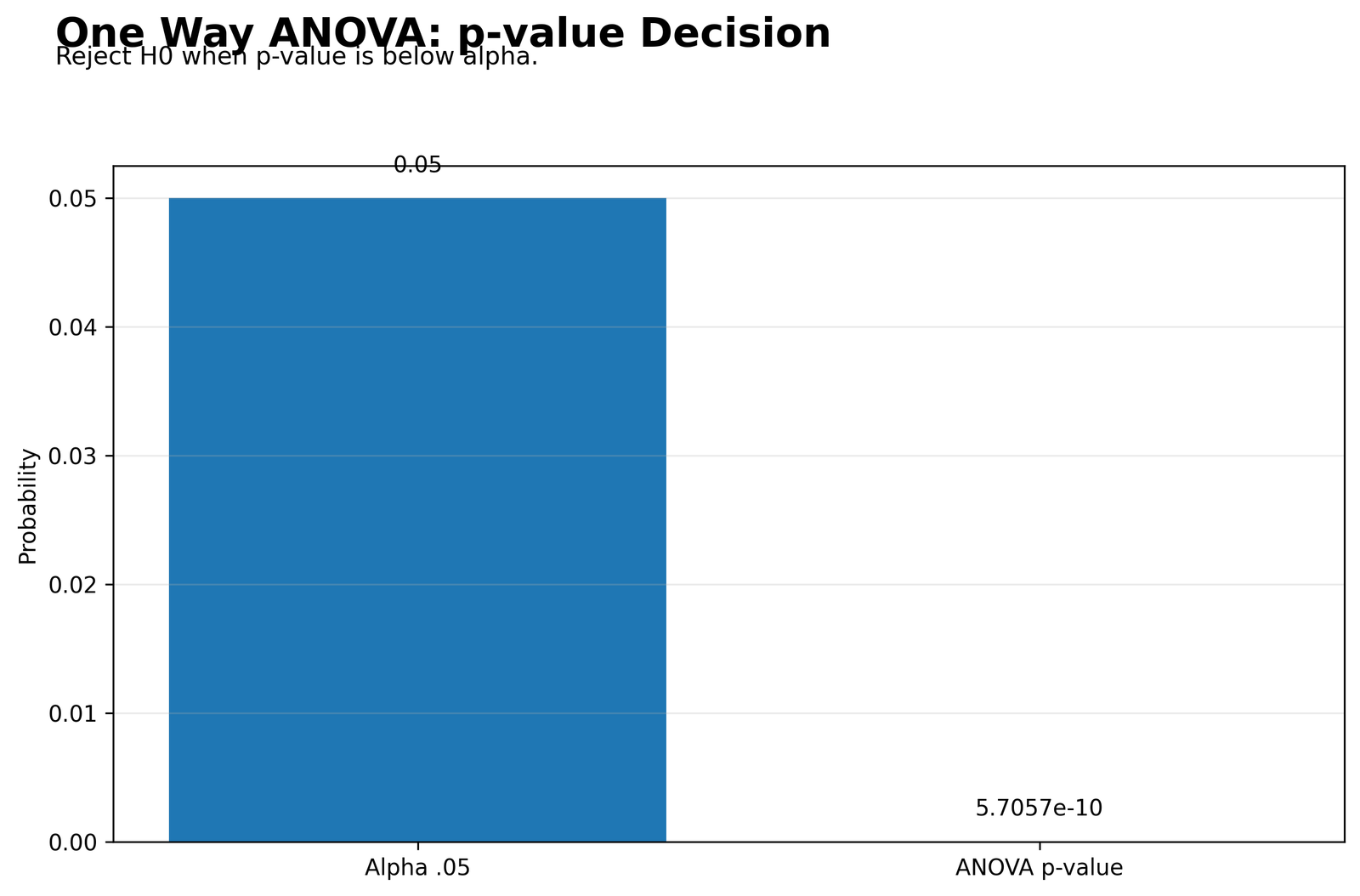
The decision chart compares alpha = .05 with the ANOVA p-value. The p-value is labelled 5.7057e-10, which is essentially zero compared with the alpha bar.
The decision is clear: reject the null hypothesis of equal studytime means. The group means are statistically different, and the result is not a borderline decision.
Python Chart 5: Residuals vs Fitted Values
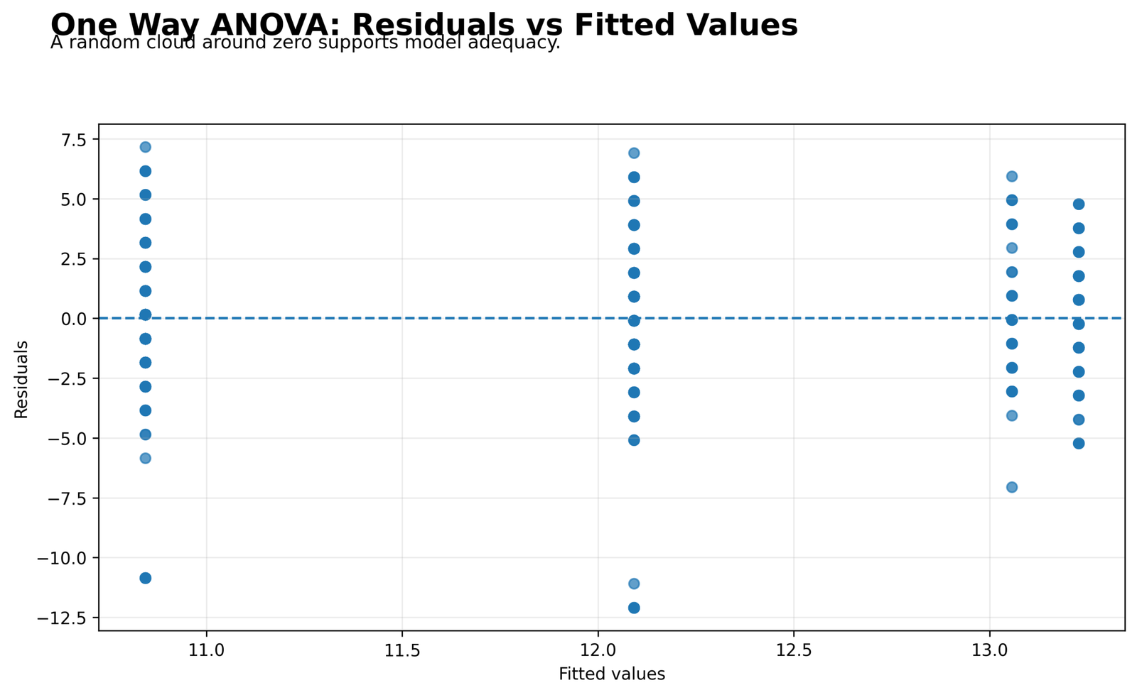
The residuals-versus-fitted chart shows vertical fitted-value bands because the model fits one mean for each studytime group. Most residuals are distributed around zero, but several negative residuals fall far below the center.
Those large negative residuals represent students whose observed G3 values were much lower than their fitted group mean. The chart does not remove the significant ANOVA result, but it shows why residual diagnostics should be discussed.
Python Chart 6: Residual Q-Q Plot
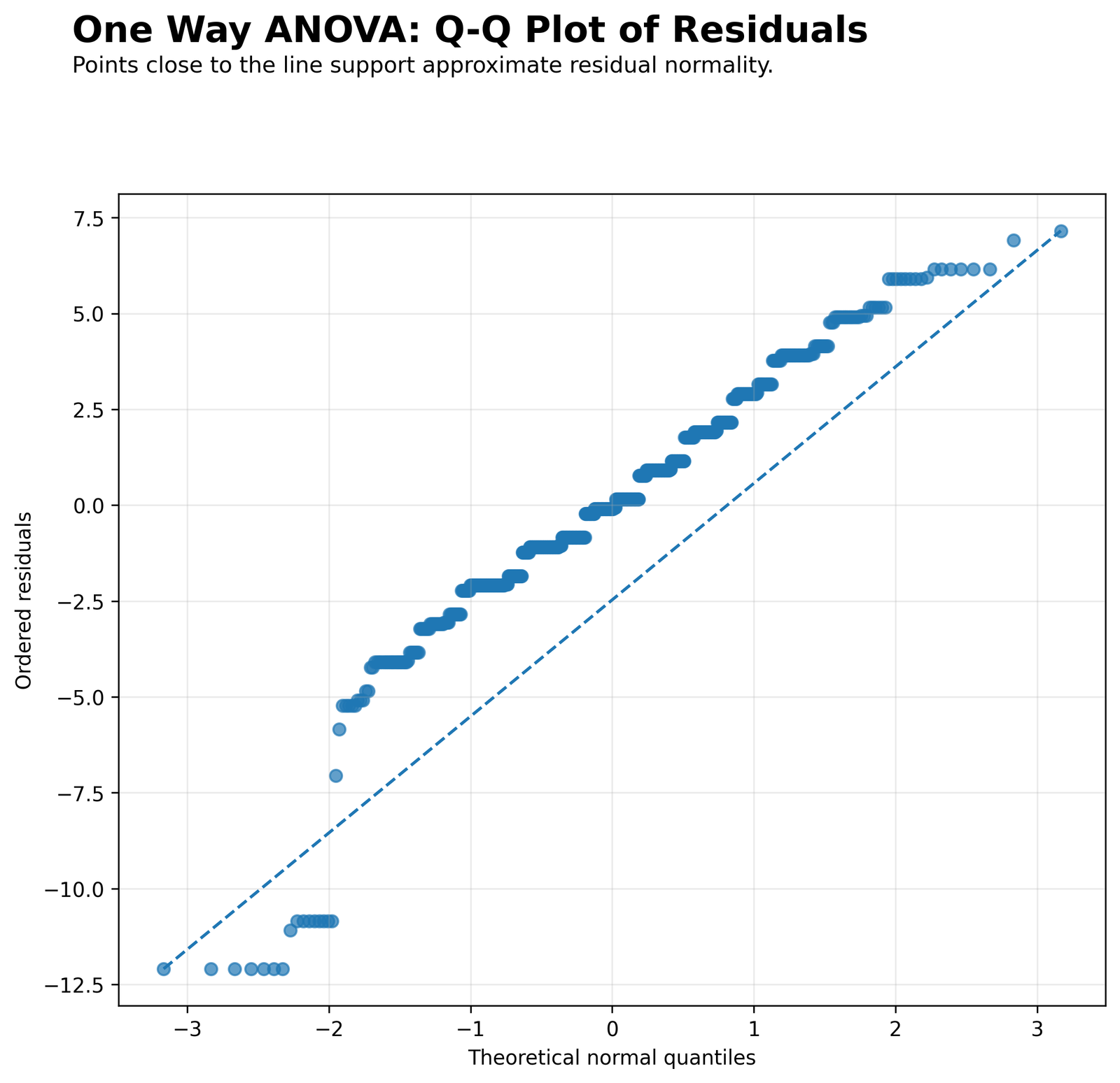
The Q-Q plot shows that the residuals are not perfectly normal. The middle points follow the reference pattern more closely, while the lower tail departs strongly from the line.
This diagnostic pattern should be reported honestly. The large sample and strong ANOVA result make the group comparison useful, but the residual normality assumption is approximate rather than perfect.
Python Chart 7: Variance Check by Group
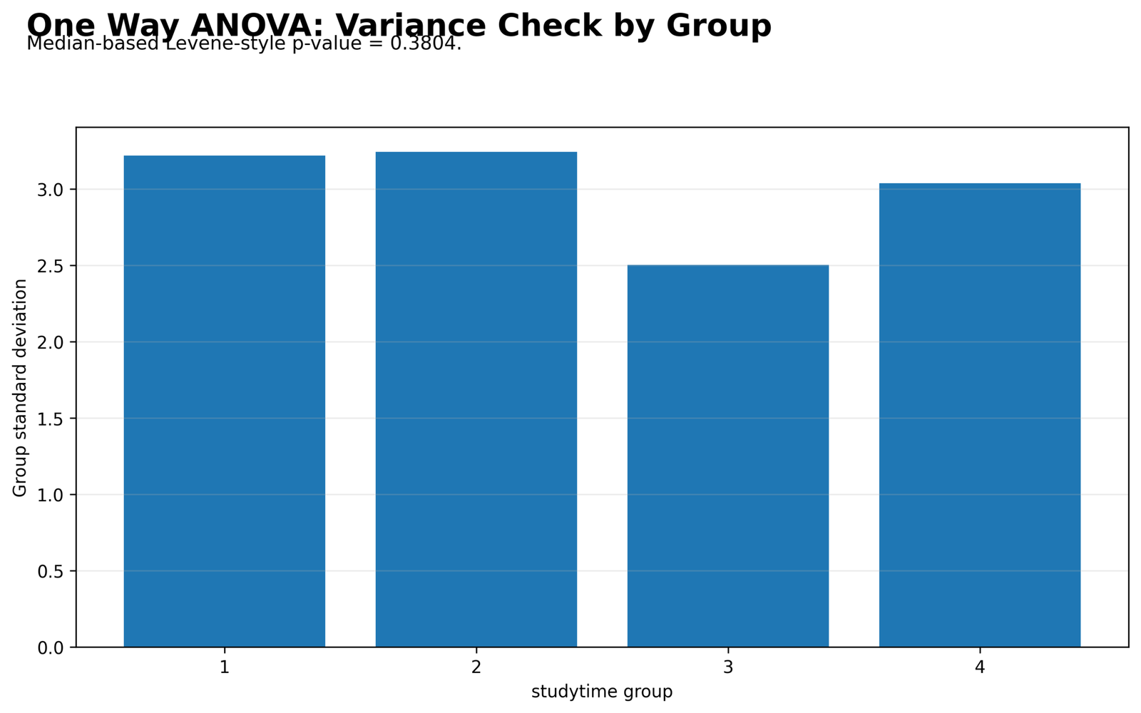
The variance chart shows group standard deviations of about 3.22, 3.24, 2.50 and 3.04. Group 3 has the smallest spread, while groups 1 and 2 have the largest spread.
The chart reports a median-based Levene-style p-value of 0.3804. Because this is above .05, the variance check does not show a serious homogeneity-of-variance problem for the ANOVA result.
Python Chart 8: ANOVA Group Summary Table
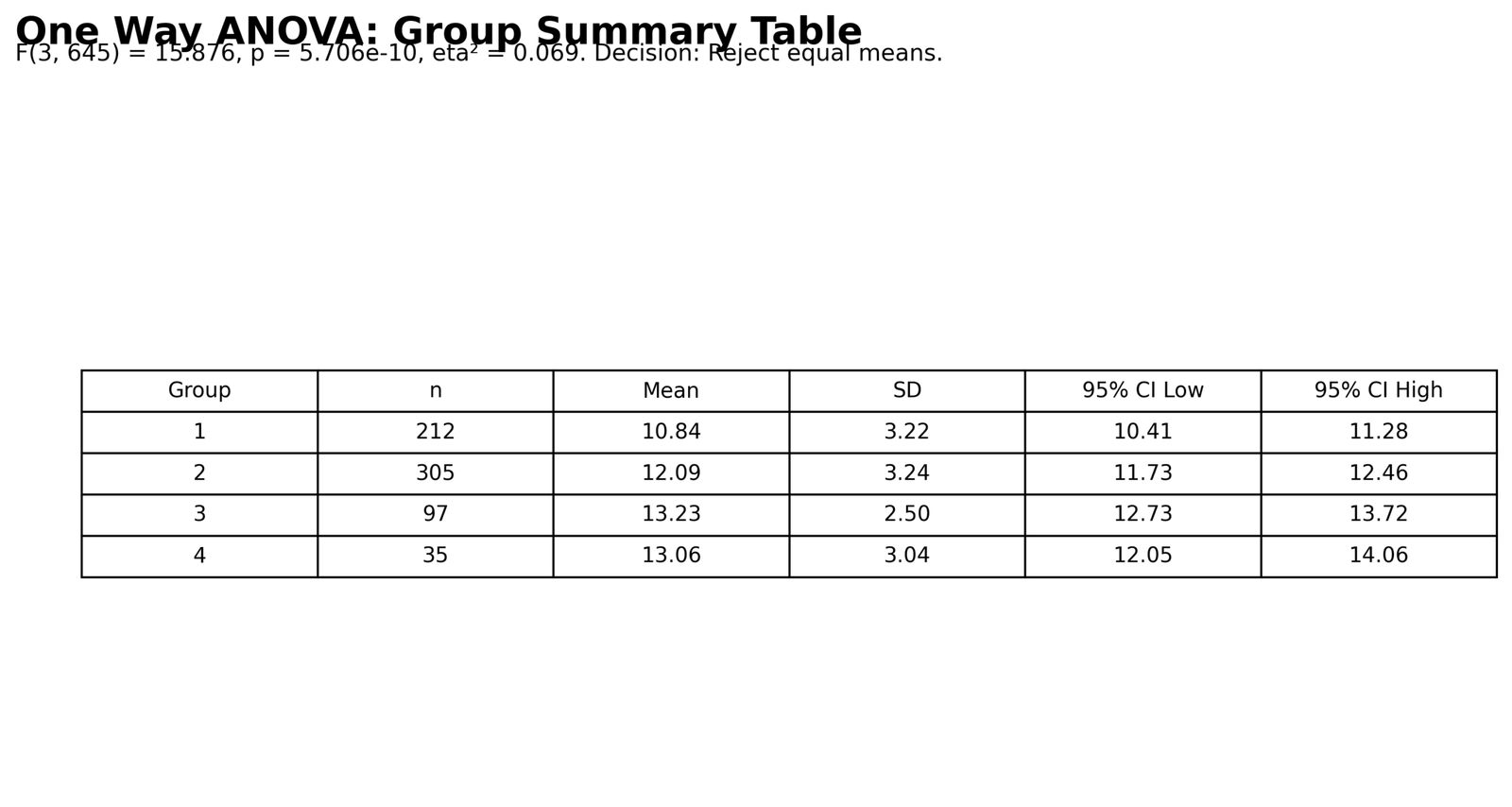
The summary table brings the main descriptive and inferential results together. It reports F(3, 645) = 15.876, p = 5.706e-10 and eta squared = 0.069.
The table confirms that group 2 is the largest group with n = 305, while group 4 is the smallest with n = 35. The means show the same pattern as the bar chart: group 1 is lowest, group 3 is highest, and group 4 remains high with the widest confidence interval.
R Chart-by-Chart Validation
The R validation charts repeat the same One Way ANOVA workflow in a second software environment. They confirm the group mean pattern, boxplot structure, F statistic decision, p-value decision, residual diagnostics, variance check and summary table.
R Chart 1: Group Mean G3 with 95% Confidence Intervals
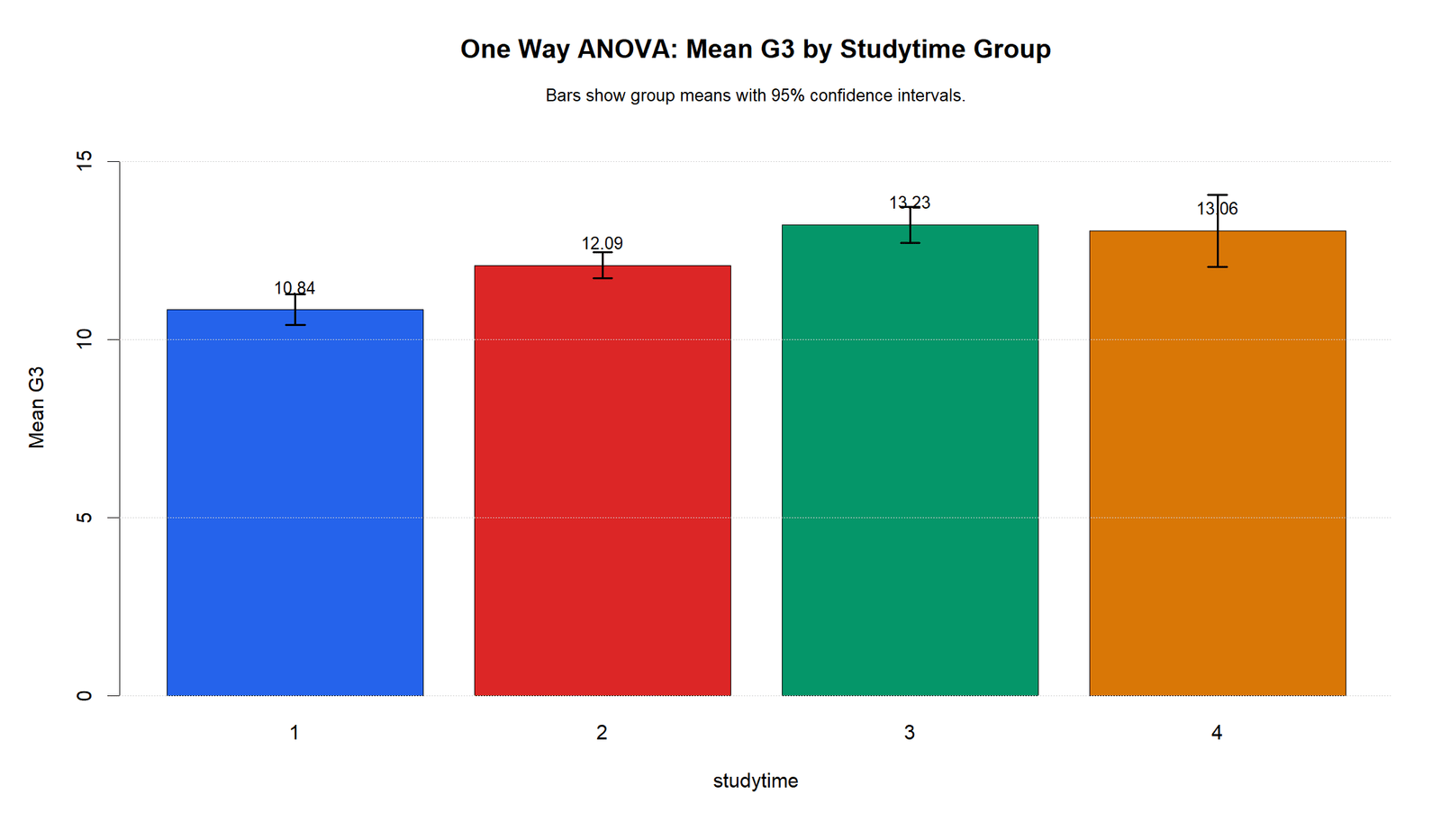
The R group mean chart confirms the Python mean pattern. Group 1 is lowest, group 2 is higher, group 3 is highest, and group 4 stays close to group 3.
This software-to-software agreement strengthens the conclusion that the studytime group mean pattern is stable and not a graphing artifact.
R Chart 2: Distribution by Studytime Group
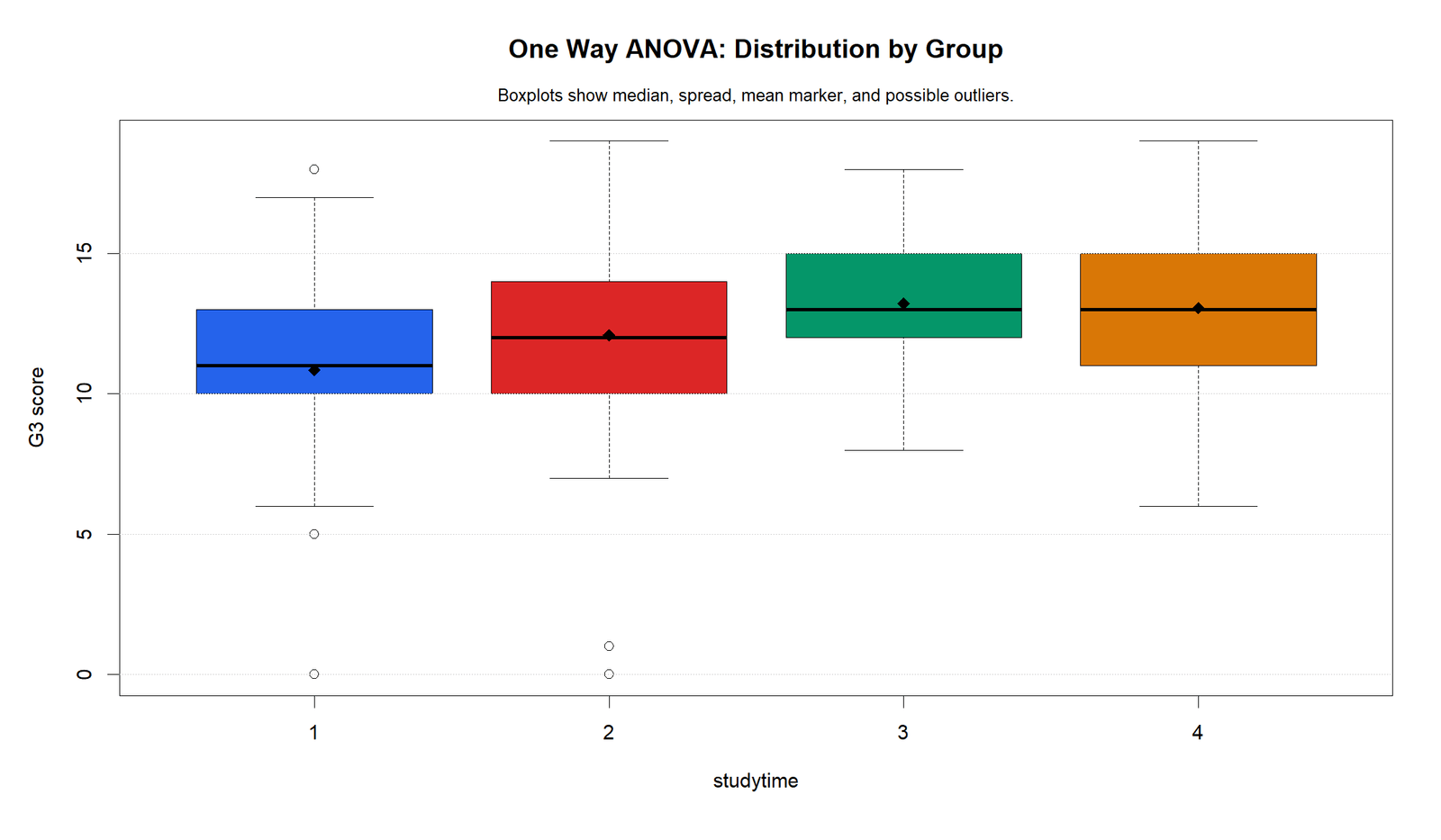
The R boxplots confirm that the higher studytime groups are centered above the lower groups. Group 1 remains the lowest distribution, while groups 3 and 4 are in the highest range.
The low outlying values remain visible, which supports the same residual diagnostic interpretation found in the Python workflow.
R Chart 3: Observed F Distribution
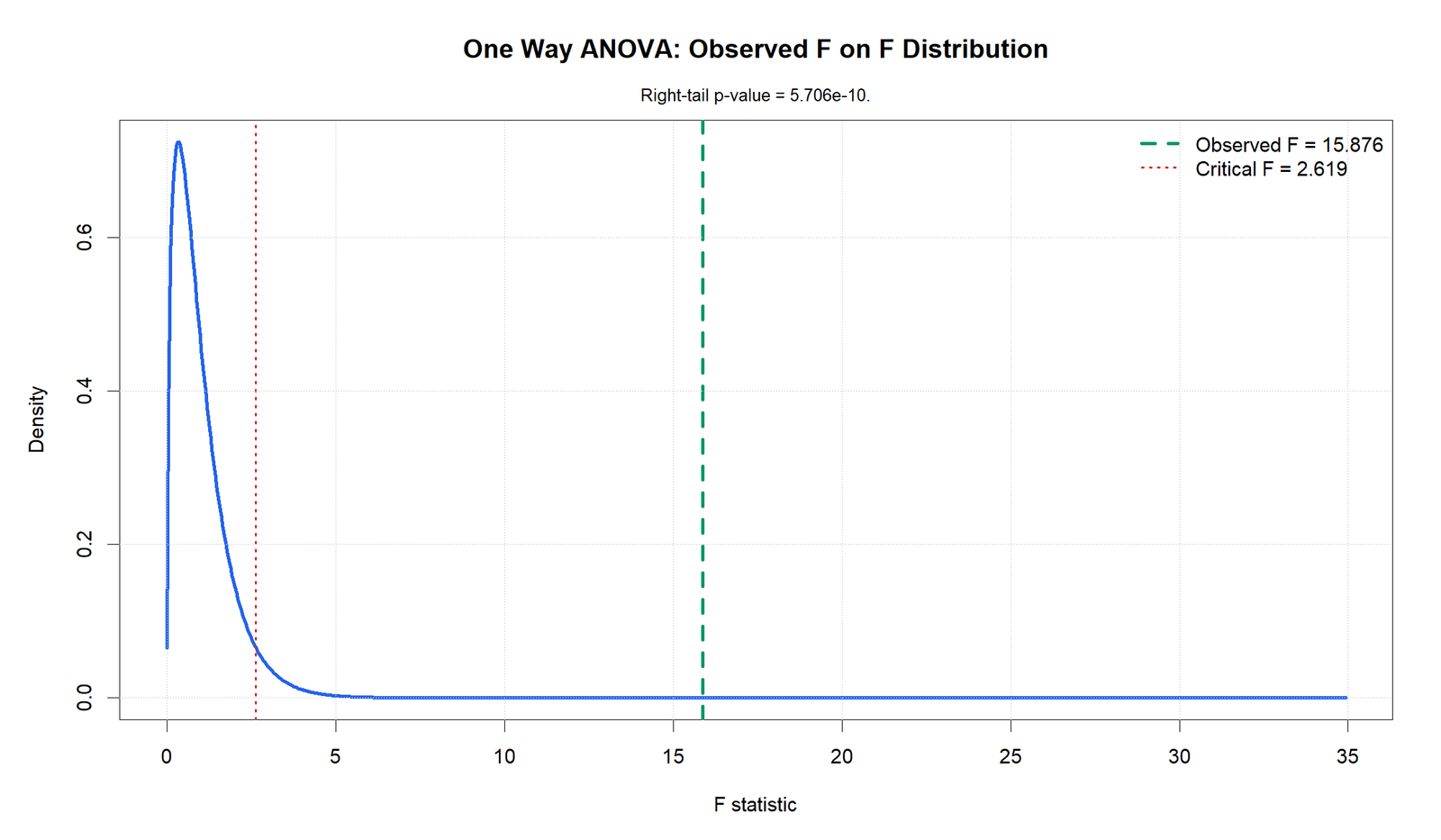
The R F distribution chart confirms that the observed F statistic is far into the right tail. This validates the formal significance decision.
The chart shows why the p-value is extremely small. The observed group differences are too large to be treated as ordinary random variation under the equal-means model.
R Chart 4: p-value Decision
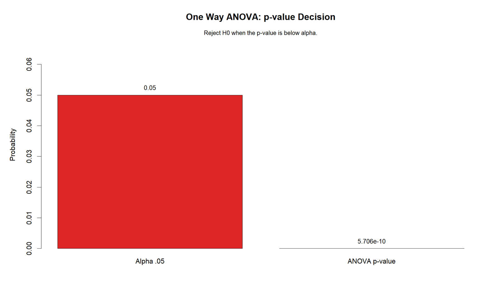
The R decision chart confirms that the ANOVA p-value is far below .05. The alpha bar is visible, while the ANOVA p-value is near the baseline.
This validates the same final decision: reject the null hypothesis and report that the studytime group means differ significantly.
R Chart 5: Residuals vs Fitted Values
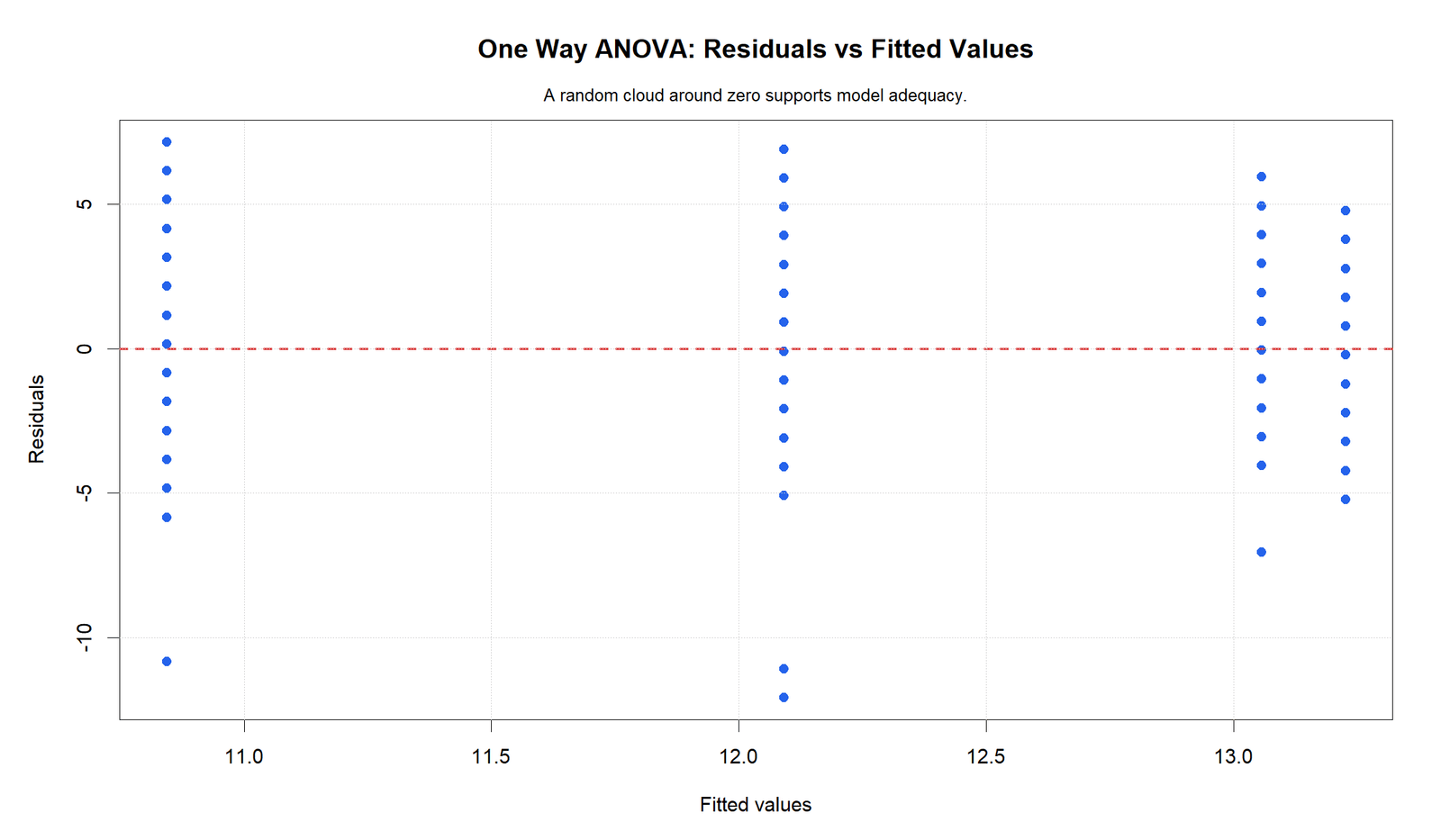
The R residuals-versus-fitted chart repeats the same diagnostic pattern. Residuals are centered around zero overall, but several negative residuals extend far below the center line.
This chart supports the same model-checking conclusion: the ANOVA group effect is clear, but residual behavior should still be reported.
R Chart 6: Residual Q-Q Plot
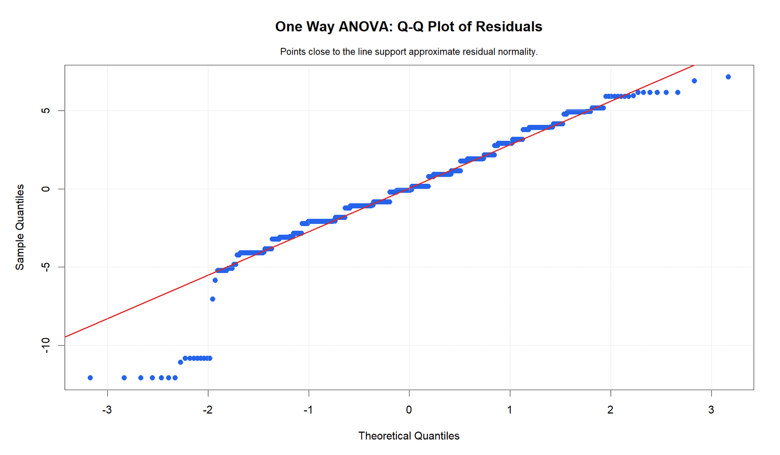
The R Q-Q plot confirms the lower-tail residual departure. The central residuals are closer to the reference line than the extreme lower-tail values.
This diagnostic agreement between Python and R means the residual issue is part of the data pattern. It should be discussed rather than ignored.
R Chart 7: Variance Check by Group
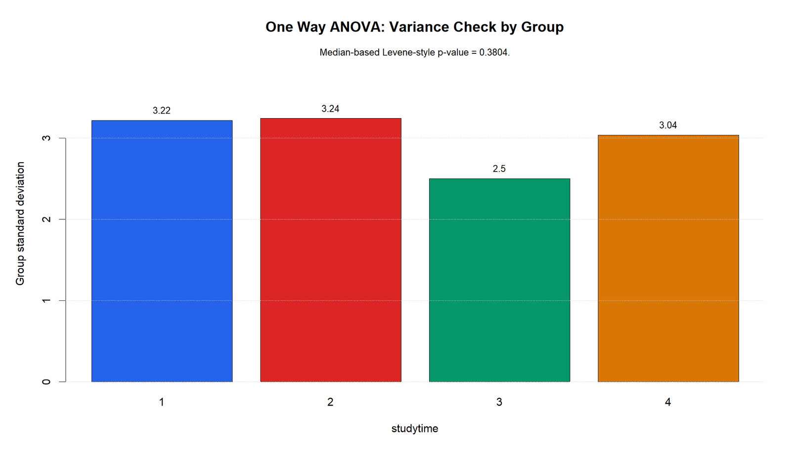
The R variance chart confirms that group 3 has the smallest standard deviation and groups 1 and 2 have larger standard deviations. The group spreads are not identical, but the Levene-style result does not show a serious violation at .05.
This supports using the standard One Way ANOVA result while still reporting the variance check.
R Chart 8: ANOVA Summary Table
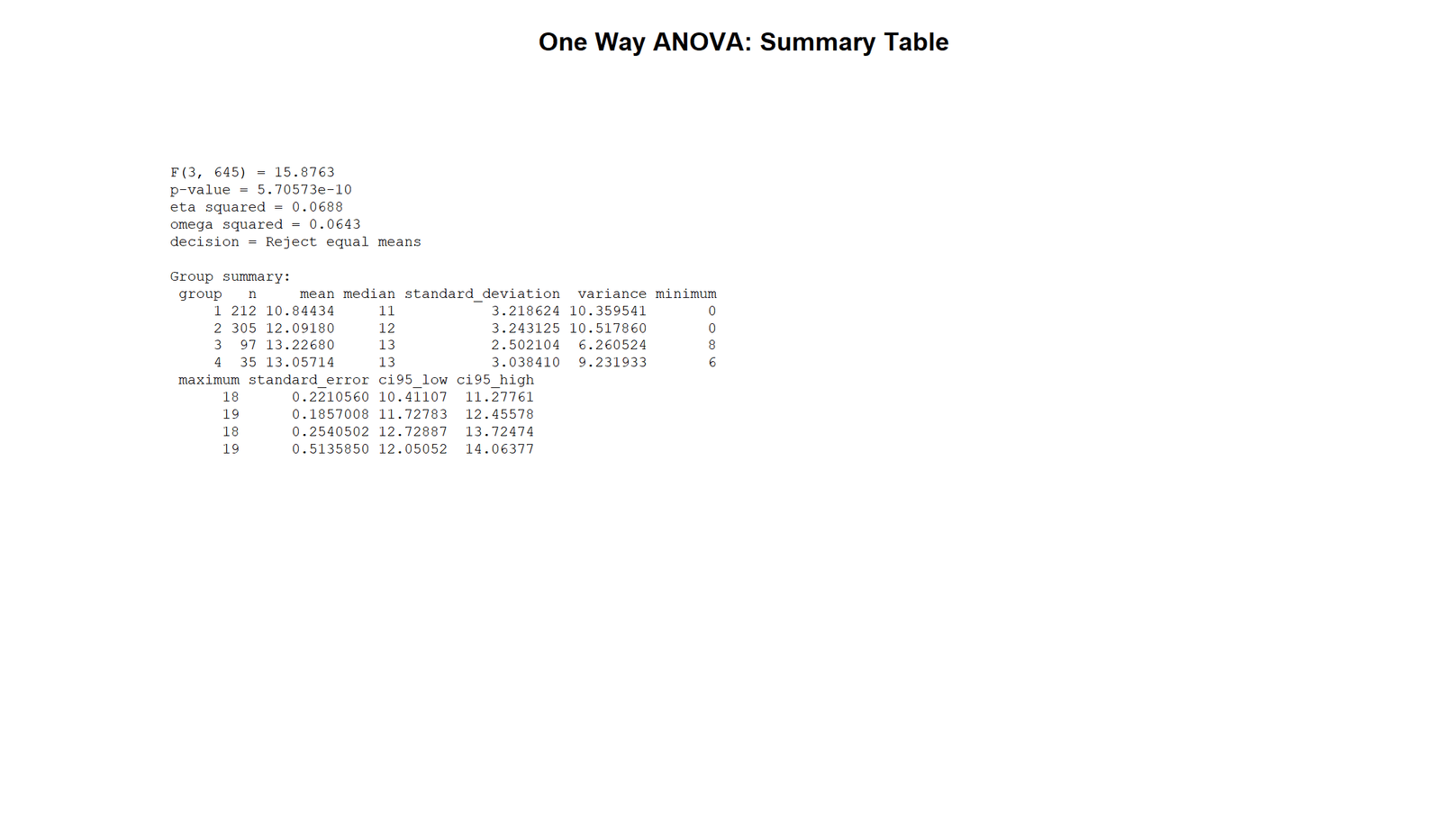
The R summary table confirms the same ANOVA conclusion: F(3, 645) = 15.876, p = 5.706e-10 and eta squared = 0.069.
The group-level statistics also match the Python table. This validates the results across both workflows and supports using the table as the compact final reporting output.
SPSS, R, Python and Excel Workflows for One Way ANOVA
The same One Way ANOVA workflow can be reproduced in SPSS, R, Python and Excel. The main requirements are one numeric dependent variable, one categorical factor with three or more groups, and independent observations.
SPSS Workflow
| Step | SPSS Menu or Syntax | Purpose |
|---|---|---|
| Open dataset | File > Open > Data | Load G3 and studytime. |
| Run One-Way ANOVA | Analyze > Compare Means > One-Way ANOVA | Compare mean G3 across studytime groups. |
| Set dependent variable | Dependent List: G3 | Define the numeric outcome. |
| Set factor | Factor: studytime | Define the grouping variable. |
| Request descriptive statistics | Options > Descriptive | Get group means, SDs and confidence intervals. |
| Request homogeneity test | Options > Homogeneity of variance test | Check equal variance assumption. |
| Post hoc tests | Post Hoc > Tukey or Games-Howell | Compare pairs of groups after significant ANOVA. |
| Export output | OUTPUT EXPORT | Save SPSS output PDF. |
R Workflow
| Step | R Action | Purpose |
|---|---|---|
| Read data | read.csv("dataset.csv") | Load the dataset. |
| Set factor | as.factor(studytime) | Define studytime as categorical. |
| Run ANOVA | aov(G3 ~ studytime) | Fit the one-way ANOVA model. |
| Read table | summary(model) | Get F statistic and p-value. |
| Effect size | Calculate eta squared | Report practical effect size. |
| Post hoc | TukeyHSD(model) | Identify pairwise group differences. |
| Diagnostics | Residual plots and Q-Q plot | Check assumptions. |
Python Workflow
| Step | Python Action | Purpose |
|---|---|---|
| Read data | pandas.read_csv() | Load G3 and studytime. |
| Fit model | ols("G3 ~ C(studytime)") | Fit one-way ANOVA model. |
| ANOVA table | sm.stats.anova_lm() | Get SS, df, F and p-value. |
| Group summaries | groupby() | Calculate n, mean, SD and confidence intervals. |
| Effect size | SS_between / SS_total | Calculate eta squared. |
| Post hoc | pairwise_tukeyhsd() | Compare group pairs. |
| Diagnostics | Residuals vs fitted and Q-Q plot | Check assumptions. |
Excel Workflow
| Excel Task | Formula or Tool | Purpose |
|---|---|---|
| Arrange data | One column per group or grouped layout | Prepare ANOVA input. |
| Enable ToolPak | File > Options > Add-ins > Analysis ToolPak | Activate ANOVA tools. |
| Run ANOVA | Data > Data Analysis > ANOVA: Single Factor | Generate F statistic and p-value. |
| Read p-value | ANOVA output table | Decide whether group means differ. |
| Calculate eta squared | =SS_between/SS_total | Report effect size. |
| Create charts | Bar chart and boxplot support | Visualize mean and distribution differences. |
Code Blocks for One Way ANOVA
SPSS Syntax for One Way ANOVA
* One Way ANOVA in SPSS.
* Dependent variable: G3.
* Factor: studytime.

TITLE "One Way ANOVA: G3 by Studytime".

ONEWAY G3 BY studytime
  /STATISTICS DESCRIPTIVES HOMOGENEITY
  /MISSING ANALYSIS
  /POSTHOC = TUKEY ALPHA(.05).

UNIANOVA G3 BY studytime
  /METHOD=SSTYPE(3)
  /INTERCEPT=INCLUDE
  /PRINT=DESCRIPTIVE ETASQ HOMOGENEITY
  /EMMEANS=TABLES(studytime)
  /CRITERIA=ALPHA(.05)
  /DESIGN=studytime.

OUTPUT EXPORT
  /CONTENTS EXPORT=VISIBLE
  /PDF DOCUMENTFILE="One-Way-ANOVA-SPSS-Output.pdf".
Python Code for One Way ANOVA
import pandas as pd
import statsmodels.api as sm
from statsmodels.formula.api import ols
from statsmodels.stats.multicomp import pairwise_tukeyhsd

df = pd.read_csv("dataset.csv")

df["G3"] = pd.to_numeric(df["G3"], errors="coerce")
df["studytime"] = df["studytime"].astype("category")

df_model = df.dropna(subset=["G3", "studytime"]).copy()

# One Way ANOVA model
model = ols("G3 ~ C(studytime)", data=df_model).fit()

anova_table = sm.stats.anova_lm(model, typ=2)
print(anova_table)

# Eta squared
ss_between = anova_table.loc["C(studytime)", "sum_sq"]
ss_error = anova_table.loc["Residual", "sum_sq"]
ss_total = ss_between + ss_error
eta_squared = ss_between / ss_total
print("Eta squared:", eta_squared)

# Group summaries
summary = (
    df_model.groupby("studytime")["G3"]
    .agg(["count", "mean", "std"])
    .reset_index()
)
print(summary)

# Tukey post hoc test
tukey = pairwise_tukeyhsd(
    endog=df_model["G3"],
    groups=df_model["studytime"],
    alpha=0.05
)
print(tukey)

# Diagnostics
df_model["fitted"] = model.fittedvalues
df_model["residual"] = model.resid
print(df_model[["G3", "studytime", "fitted", "residual"]].head())
R Code for One Way ANOVA
# One Way ANOVA in R

library(tidyverse)

df <- read.csv("dataset.csv")

df$G3 <- as.numeric(df$G3)
df$studytime <- as.factor(df$studytime)

df_model <- df %>%
  select(G3, studytime) %>%
  drop_na()

# One Way ANOVA
model <- aov(G3 ~ studytime, data = df_model)

summary(model)

# Group summaries
df_model %>%
  group_by(studytime) %>%
  summarise(
    n = n(),
    mean = mean(G3),
    sd = sd(G3),
    .groups = "drop"
  )

# Eta squared
anova_table <- summary(model)[[1]]
ss_between <- anova_table["studytime", "Sum Sq"]
ss_error <- anova_table["Residuals", "Sum Sq"]
eta_squared <- ss_between / (ss_between + ss_error)
eta_squared

# Tukey post hoc test
TukeyHSD(model)

# Diagnostics
plot(model)
Excel Formulas for One Way ANOVA
Step 1:
Arrange G3 scores by studytime group.

Step 2:
Enable Analysis ToolPak:
File > Options > Add-ins > Excel Add-ins > Analysis ToolPak.

Step 3:
Run:
Data > Data Analysis > ANOVA: Single Factor.

Step 4:
Read the ANOVA output:
F statistic
p-value
F critical
Between Groups SS
Within Groups SS
Total SS

Step 5:
Decision rule:
If p-value < 0.05, reject equal group means.

Step 6:
Eta squared:
=SS_between / SS_total

Step 7:
Report:
F(df_between, df_within) = value, p = value, eta squared = value.
APA Reporting Wording
When reporting One Way ANOVA, include the factor, dependent variable, F statistic, degrees of freedom, p-value, effect size and a short explanation of the group mean pattern.
APA-style report: A one-way ANOVA was conducted to compare G3 final grade across four studytime groups. The result was statistically significant, F(3, 645) = 15.876, p = 5.706e-10, η² = 0.069. Mean G3 increased from studytime group 1 to group 3, with group 4 remaining high. The homogeneity-of-variance check did not show a serious variance problem, Levene-style p = 0.3804, although residual diagnostics showed lower-tail departures.
Short reporting version: Studytime had a significant effect on G3, F(3, 645) = 15.876, p < .001, η² = 0.069. Group 1 had the lowest mean, while groups 3 and 4 had the highest means.
Common Mistakes
| Mistake | Why It Is Wrong | Correct Practice |
|---|---|---|
| Using many t tests instead of ANOVA | Multiple t tests inflate Type I error. | Use One Way ANOVA for three or more groups. |
| Reporting only p-value | The p-value does not show practical size. | Report eta squared or another effect size. |
| Assuming ANOVA identifies all pairwise differences | ANOVA only says at least one mean differs. | Use post hoc tests for pairwise comparisons. |
| Ignoring variance checks | ANOVA assumes reasonably similar group variances. | Report Levene test or use robust alternatives when needed. |
| Ignoring residual diagnostics | The Q-Q plot shows lower-tail departure. | Discuss diagnostics and review Q-Q Plot Normality Check. |
| Calling eta squared = 0.069 huge | The effect is meaningful but not dominant. | Report it as a medium-style effect in practical interpretation. |
When to Use One Way ANOVA
Use One Way ANOVA when you have one categorical independent variable with three or more independent groups and one numeric dependent variable. In this example, studytime has four groups, and G3 is numeric.
| Situation | Use One Way ANOVA? | Reporting Note |
|---|---|---|
| One factor with three or more groups | Yes | Report F, p and effect size. |
| Only two independent groups | Use independent samples t test | See Independent Samples T Test. |
| Two categorical factors | Use factorial ANOVA | See Factorial ANOVA. |
| Need to control a covariate | Use ANCOVA | See ANCOVA. |
| Variances are strongly unequal | Use Welch ANOVA or robust ANOVA | Review Brown Forsythe ANOVA. |
One Way ANOVA should be compared with Fixed Effects ANOVA, Factorial ANOVA, Balanced ANOVA, Brown Forsythe ANOVA, ANOVA Assumptions, T Test vs ANOVA, and Welch’s T Test.
Downloads and Resources for One Way ANOVA
Use these resources to reproduce the One Way ANOVA workflow. The Python report, R report and SPSS output PDF are included as verification files. Script and workbook placeholders can be replaced after the final downloadable files are uploaded to the WordPress Media Library.
Download Dataset
Practice dataset with G3 and studytime variables.
Download One Way ANOVA Python Report PDF
Python report PDF for group means, F statistic, p-value, diagnostics and summary table.
Download One Way ANOVA R Report PDF
R validation PDF for group means, F decision, variance check and residual diagnostics.
Download One Way ANOVA SPSS Output PDF
SPSS output PDF for ANOVA interpretation and reporting.
Download Python Script
Python code for One Way ANOVA, post hoc test, eta squared and diagnostics.
Download R Script and Excel Workbook
R workflow and Excel support workbook for One Way ANOVA summaries.
FAQs About One Way ANOVA
What is One Way ANOVA?
One Way ANOVA is a statistical test used to compare the means of three or more independent groups on one numeric outcome.
What variables were used in this example?
The dependent variable was G3 final grade, and the grouping factor was studytime with four groups.
What was the One Way ANOVA result?
The result was F(3, 645) = 15.876, p = 5.706e-10.
Was the result statistically significant?
Yes. The p-value was far below .05, so the equal-means null hypothesis was rejected.
What were the group means?
The group means were 10.84, 12.09, 13.23 and 13.06 for studytime groups 1 through 4.
What was eta squared?
Eta squared was 0.069, meaning studytime explained about 6.9% of observed G3 variance.
What did the variance check show?
The median-based Levene-style p-value was 0.3804, which did not show a serious variance problem at alpha = .05.
Does One Way ANOVA show which groups differ?
No. One Way ANOVA shows that at least one mean differs. Post hoc tests are needed to identify specific pairwise group differences.
Can One Way ANOVA be done in Excel?
Yes. Excel can run One Way ANOVA using the Data Analysis ToolPak and ANOVA: Single Factor option.
How do I report this One Way ANOVA in APA style?
A concise report is: Studytime had a significant effect on G3, F(3, 645) = 15.876, p < .001, η² = 0.069.

