
.sgn-wrap{–ink:#172033;–muted:#607083;–navy:#123b5d;–blue:#176ea6;–teal:#087f6b;–amber:#b86b10;–rose:#a33a54;–line:#d8e3ea;–soft:#f5f9fc;–soft2:#eefbf8;–warn:#fff7e8;–danger:#fff1f2;–code:#101828;max-width:1120px;margin:0 auto;color:var(–ink);font-family:system-ui,-apple-system,BlinkMacSystemFont,”Segoe UI”,Arial,sans-serif;line-height:1.76}
.sgn-wrap *{box-sizing:border-box}.sgn-wrap h1,.sgn-wrap h2,.sgn-wrap h3,.sgn-wrap h4{line-height:1.25}.sgn-wrap h2{font-size:30px;color:var(–navy);margin:0 0 16px}.sgn-wrap h3{font-size:23px;color:#245877;margin:28px 0 12px}.sgn-wrap h4{font-size:18px;color:#263c52;margin:22px 0 9px}.sgn-wrap p{margin:0 0 16px}.sgn-wrap a{color:#0b6598;text-decoration:underline}.sgn-wrap li{margin:7px 0}
.sgn-hero{padding:36px;border:1px solid var(–line);border-radius:26px;background:linear-gradient(135deg,#eef7fb 0%,#fff 52%,#fff4e7 100%);box-shadow:0 14px 36px rgba(24,59,86,.08);margin:14px 0 26px}
.sgn-kicker{display:inline-flex;align-items:center;gap:8px;padding:7px 13px;border-radius:999px;background:#e7f6f3;border:1px solid #bce5dc;color:#075f52;font-size:13px;font-weight:800;letter-spacing:.04em;text-transform:uppercase;margin-bottom:15px}
.sgn-hero h1{font-size:43px;color:#102e46;margin:0 0 16px}.sgn-hero p{font-size:20px;color:#2b3b4e;margin:0}.sgn-badges{display:flex;flex-wrap:wrap;gap:10px;margin-top:22px}.sgn-badge{padding:8px 12px;border-radius:999px;border:1px solid var(–line);background:#fff;font-weight:750;font-size:14px}
.sgn-ad{padding:18px;border:1px dashed #aebbc8;border-radius:16px;text-align:center;color:#718096;background:#fcfdfe;margin:27px 0}.sgn-ad span{display:block;font-size:11px;text-transform:uppercase;letter-spacing:.1em;margin-bottom:4px}
.sgn-section{background:#fff;border:1px solid var(–line);border-radius:22px;padding:25px;margin:24px 0;box-shadow:0 8px 24px rgba(15,23,42,.035)}
.sgn-note{background:#f5f9fd;border-left:5px solid var(–navy);border-radius:16px;padding:18px 20px;margin:19px 0}.sgn-success{background:#ecfdf5;border:1px solid #bbf7d0;border-radius:17px;padding:18px 20px;margin:19px 0}.sgn-warning{background:var(–warn);border:1px solid #f1d19b;border-radius:17px;padding:18px 20px;margin:19px 0}.sgn-danger{background:var(–danger);border:1px solid #fecdd3;border-radius:17px;padding:18px 20px;margin:19px 0}
.sgn-stat-grid{display:grid;grid-template-columns:repeat(4,minmax(0,1fr));gap:14px;margin:20px 0}.sgn-stat{padding:17px;border:1px solid var(–line);border-radius:17px;background:var(–soft)}.sgn-stat small{display:block;color:var(–muted);margin-bottom:6px}.sgn-stat strong{display:block;font-size:23px;color:var(–navy)}
.sgn-result-grid{display:grid;grid-template-columns:1fr 1fr;gap:18px;margin:20px 0}.sgn-result{border:1px solid var(–line);border-radius:19px;padding:20px}.sgn-result.method{background:#f1f8fc}.sgn-result.meaning{background:#f0fbf7}.sgn-result h3{margin:0 0 8px}.sgn-result ul{margin:10px 0 0;padding-left:20px}
.sgn-toc{columns:2;column-gap:34px;margin:0;padding-left:20px}.sgn-toc li{break-inside:avoid;margin:8px 0}
.sgn-problem-grid{display:grid;grid-template-columns:repeat(3,minmax(0,1fr));gap:15px}.sgn-problem{border:1px solid var(–line);border-radius:18px;padding:18px;background:var(–soft)}.sgn-problem strong{display:block;font-size:20px;color:var(–navy);margin-bottom:5px}.sgn-problem span{color:var(–muted)}
.sgn-flow{display:grid;grid-template-columns:1fr auto 1fr auto 1fr;gap:12px;align-items:stretch;margin:22px 0}.sgn-step{border:1px solid var(–line);border-radius:18px;padding:19px;background:#fff}.sgn-step b{display:block;color:var(–teal);font-size:13px;text-transform:uppercase;letter-spacing:.05em;margin-bottom:7px}.sgn-arrow{display:flex;align-items:center;font-size:28px;color:#8aa0b2;font-weight:800}
.sgn-formula{padding:18px;border:1px solid var(–line);border-radius:17px;text-align:center;background:#f7f9fc;font-weight:800;font-size:19px;color:var(–navy);margin:18px 0;overflow-x:auto}
.sgn-table-wrap{overflow-x:auto;border:1px solid var(–line);border-radius:18px;margin:18px 0}.sgn-table{width:100%;min-width:880px;border-collapse:collapse;background:#fff}.sgn-table th{background:#edf5f9;color:#163d58;text-align:left;padding:12px;border-bottom:1px solid var(–line)}.sgn-table td{padding:12px;border-bottom:1px solid #edf1f4;vertical-align:top}.sgn-table tr:last-child td{border-bottom:none}
.sgn-decision-grid{display:grid;grid-template-columns:repeat(2,minmax(0,1fr));gap:16px;margin:20px 0}.sgn-decision{border:1px solid var(–line);border-radius:18px;padding:19px;background:#fff}.sgn-decision h3{margin-top:0}.sgn-decision.use{border-top:5px solid var(–teal)}.sgn-decision.avoid{border-top:5px solid var(–amber)}
.sgn-method-grid{display:grid;grid-template-columns:repeat(4,minmax(0,1fr));gap:13px;margin:20px 0}.sgn-method{border:1px solid var(–line);border-radius:17px;padding:17px;background:#fff}.sgn-method strong{display:block;color:var(–navy);font-size:18px;margin-bottom:7px}.sgn-method p{font-size:14px;color:#405368;margin:0}
.sgn-chart-story{border-top:1px solid var(–line);padding:30px 0 8px}.sgn-chart-story:first-of-type{border-top:none;padding-top:4px}.sgn-figure{margin:16px 0 18px;border:1px solid var(–line);border-radius:20px;overflow:hidden;background:#fff}.sgn-figure img{display:block;width:100%;height:auto}.sgn-figure figcaption{padding:13px 16px;background:#fbfdff;border-top:1px solid var(–line);color:var(–muted);font-size:14px}
.sgn-insight-grid{display:grid;grid-template-columns:1fr 1fr;gap:13px}.sgn-insight{border:1px solid var(–line);border-radius:16px;padding:16px;background:#fff}.sgn-insight span{display:block;font-size:12px;font-weight:850;letter-spacing:.06em;text-transform:uppercase;color:var(–teal);margin-bottom:7px}.sgn-insight p{margin:0}.sgn-next{margin:13px 0 0;padding:13px 15px;border-radius:14px;background:#f3f7fb;color:#405368;font-size:14px}
.sgn-metric-grid{display:grid;grid-template-columns:repeat(3,minmax(0,1fr));gap:14px}.sgn-metric{border:1px solid var(–line);border-radius:17px;padding:17px;background:#fff}.sgn-metric b{display:block;color:var(–navy);margin-bottom:6px}.sgn-metric strong{font-size:20px;color:var(–teal)}
.sgn-software-grid{display:grid;grid-template-columns:repeat(2,minmax(0,1fr));gap:16px}.sgn-software{border:1px solid var(–line);border-radius:18px;padding:19px}.sgn-software h3{margin:0 0 8px}.sgn-software ul{padding-left:19px;margin:8px 0}
.sgn-details details{border:1px solid var(–line);border-radius:15px;padding:14px 16px;margin:11px 0;background:#fff}.sgn-details summary{cursor:pointer;font-weight:850;color:var(–navy)}.sgn-details details>div{padding-top:13px}
.sgn-code{background:var(–code);color:#e5e7eb;border-radius:17px;padding:17px;overflow-x:auto;font-size:13.5px;line-height:1.62}.sgn-code code{font-family:Consolas,Monaco,”Courier New”,monospace}
.sgn-two-col{display:grid;grid-template-columns:1fr 1fr;gap:18px}.sgn-list-card{border:1px solid var(–line);border-radius:18px;padding:19px;background:#fff}.sgn-list-card h3{margin:0 0 9px}.sgn-list-card ul{padding-left:20px;margin:0}
.sgn-apa-grid{display:grid;grid-template-columns:1fr 1fr;gap:16px;margin:18px 0}.sgn-report{border:1px solid var(–line);border-radius:18px;padding:19px;background:#fff}.sgn-report h3{margin:0 0 10px}.sgn-copy{border-left:5px solid var(–teal);background:#f0fbf7;border-radius:15px;padding:17px 19px;margin:14px 0}.sgn-copy p:last-child{margin-bottom:0}.sgn-template{border:1px dashed #9fb0bf;border-radius:15px;background:#fbfdff;padding:16px;margin:12px 0}.sgn-template code{white-space:normal;color:#20364a;font-family:inherit}
.sgn-r-pair{margin:28px 0 34px;padding:20px;border:1px solid var(–line);border-radius:21px;background:#fbfdff}.sgn-r-pair-title{margin:0 0 15px;font-size:17px;color:var(–navy);font-weight:850}.sgn-r-chart-row{display:grid;grid-template-columns:repeat(2,minmax(0,1fr));gap:18px;align-items:start}.sgn-r-chart-box{border:1px solid var(–line);border-radius:18px;overflow:hidden;background:#fff}.sgn-r-chart-box figure{margin:0}.sgn-r-chart-box img{display:block;width:100%;height:auto}.sgn-r-chart-box figcaption{padding:12px 14px;background:#f7fafc;border-top:1px solid var(–line);color:var(–muted);font-size:13px}.sgn-r-explanation-row{display:grid;grid-template-columns:repeat(2,minmax(0,1fr));gap:18px;margin-top:14px}.sgn-r-explanation{border:1px solid var(–line);border-radius:17px;padding:17px;background:#fff}.sgn-r-explanation h3{font-size:19px;margin:0 0 9px}.sgn-r-label{display:block;font-size:12px;font-weight:850;letter-spacing:.06em;text-transform:uppercase;color:var(–teal);margin-bottom:6px}.sgn-r-check{padding:11px 13px;border-radius:13px;background:#eef7fb;color:#405368;font-size:13px;margin-top:10px}
.sgn-download-grid{display:grid;grid-template-columns:repeat(2,minmax(0,1fr));gap:14px}.sgn-download{display:block;text-decoration:none!important;border:1px solid var(–line);border-radius:17px;padding:18px;background:#fff}.sgn-download strong{display:block;color:var(–navy);font-size:18px;margin-bottom:5px}.sgn-download span{color:var(–muted);font-size:14px}.sgn-related{display:grid;grid-template-columns:repeat(2,minmax(0,1fr));gap:11px}.sgn-related a{display:block;padding:12px 14px;border:1px solid var(–line);border-radius:14px;background:#f8fafc;text-decoration:none}.sgn-faq details{border:1px solid var(–line);border-radius:15px;padding:15px 17px;margin:10px 0}.sgn-faq summary{cursor:pointer;font-weight:850;color:var(–navy)}.sgn-faq p{margin-top:11px}
html{scroll-behavior:smooth}.sgn-top-anchor{position:absolute;top:0;left:0;width:1px;height:1px;overflow:hidden}.sgn-back-to-top{position:fixed;right:22px;bottom:24px;width:48px;height:48px;display:flex;align-items:center;justify-content:center;border-radius:50%;background:var(–navy);color:#fff!important;text-decoration:none!important;font-size:25px;font-weight:900;box-shadow:0 10px 24px rgba(15,23,42,.24);z-index:9999;border:2px solid rgba(255,255,255,.85)}.sgn-back-to-top:hover{background:var(–teal);transform:translateY(-3px)}.sgn-back-to-top span{position:absolute;width:1px;height:1px;overflow:hidden;clip:rect(0,0,0,0)}
@media(max-width:900px){.sgn-method-grid{grid-template-columns:repeat(2,1fr)}.sgn-stat-grid,.sgn-metric-grid{grid-template-columns:repeat(2,1fr)}.sgn-result-grid,.sgn-two-col,.sgn-software-grid,.sgn-download-grid,.sgn-related,.sgn-insight-grid,.sgn-apa-grid,.sgn-decision-grid,.sgn-r-chart-row,.sgn-r-explanation-row{grid-template-columns:1fr}.sgn-flow{grid-template-columns:1fr}.sgn-arrow{justify-content:center;transform:rotate(90deg)}.sgn-toc{columns:1}.sgn-problem-grid{grid-template-columns:1fr}.sgn-hero h1{font-size:34px}}
@media(max-width:540px){.sgn-stat-grid,.sgn-metric-grid,.sgn-method-grid{grid-template-columns:1fr}.sgn-section,.sgn-hero{padding:21px}.sgn-hero h1{font-size:29px}.sgn-hero p{font-size:17px}.sgn-wrap h2{font-size:25px}.sgn-back-to-top{right:15px;bottom:18px;width:44px;height:44px}}
/* Readable APA templates: deliberately avoid theme styling. */
.sgn-template{
border:1px dashed #9fb0bf!important;
border-radius:15px!important;
background:#fbfdff!important;
padding:17px 19px!important;
margin:13px 0 20px!important;
color:#20364a!important;
box-shadow:none!important;
}
.sgn-template,
.sgn-template *{
color:#20364a!important;
background:transparent!important;
text-shadow:none!important;
box-shadow:none!important;
}
.sgn-template-text{
display:block!important;
margin:0!important;
padding:0!important;
border:0!important;
font-family:system-ui,-apple-system,BlinkMacSystemFont,"Segoe UI",Arial,sans-serif!important;
font-size:16px!important;
font-weight:400!important;
line-height:1.78!important;
white-space:normal!important;
word-break:normal!important;
overflow-wrap:anywhere!important;
}
/* Final APA reporting cards */
.sgn-apa-template-intro{
display:flex;
align-items:flex-start;
gap:12px;
padding:15px 17px;
margin:16px 0 18px;
border:1px solid #c9d9e5;
border-radius:15px;
background:#f5faff;
color:#29435a
}
.sgn-apa-template-intro strong{color:var(--navy)}
.sgn-apa-template-grid{
display:grid;
grid-template-columns:repeat(2,minmax(0,1fr));
gap:16px;
margin:16px 0 24px
}
.sgn-apa-template-card{
border:1px solid var(--line);
border-radius:19px;
padding:19px;
background:#fff;
box-shadow:0 5px 16px rgba(15,23,42,.035)
}
.sgn-apa-template-card.directional{grid-column:1/-1}
.sgn-apa-template-head{
display:flex;
flex-wrap:wrap;
align-items:center;
gap:10px;
margin-bottom:13px
}
.sgn-apa-template-head h4{
margin:0;
color:var(--navy);
font-size:20px
}
.sgn-apa-status{
display:inline-flex;
align-items:center;
border-radius:999px;
padding:5px 10px;
font-size:12px;
line-height:1.2;
font-weight:850;
letter-spacing:.035em;
text-transform:uppercase
}
.sgn-apa-status.ns{background:#eef4f8;color:#39556b;border:1px solid #cbd8e1}
.sgn-apa-status.sig{background:#ecfdf5;color:#076451;border:1px solid #b7e8da}
.sgn-apa-status.one{background:#fff7e8;color:#8a520a;border:1px solid #efcf98}
.sgn-apa-template-copy{
border-left:5px solid var(--blue);
border-radius:14px;
background:#f8fbfe;
padding:16px 17px;
color:#20364a
}
.sgn-apa-template-card.sig-card .sgn-apa-template-copy{border-left-color:var(--teal)}
.sgn-apa-template-card.directional .sgn-apa-template-copy{border-left-color:var(--amber)}
.sgn-apa-template-copy p{
margin:0 0 11px!important;
color:#20364a!important;
font-size:16px!important;
line-height:1.72!important
}
.sgn-apa-template-copy p:last-child{margin-bottom:0!important}
.sgn-slot{
display:inline-block;
border:1px solid #b9d2e3;
border-radius:7px;
background:#eaf5fc;
color:#164e72;
padding:1px 6px;
margin:1px 1px;
font-weight:750;
white-space:nowrap
}
.sgn-apa-template-card.sig-card .sgn-slot{
border-color:#b6dfd4;
background:#eaf9f5;
color:#086653
}
.sgn-apa-template-card.directional .sgn-slot{
border-color:#e3c68d;
background:#fff5df;
color:#87510b
}
.sgn-template-tip{
display:block;
margin-top:11px;
color:var(--muted);
font-size:13px
}
/* One presentation for charts shared by Python and R */
.sgn-cross-software{
padding:16px 18px;
border:1px solid #c8dfd8;
border-radius:16px;
background:#f0fbf7;
margin:16px 0 22px;
color:#284b43
}
.sgn-chart-badge{
display:inline-flex;
margin-left:8px;
padding:4px 9px;
border-radius:999px;
border:1px solid #c8d8e3;
background:#f3f8fb;
color:#36566d;
font-size:11px;
font-weight:800;
letter-spacing:.035em;
text-transform:uppercase;
vertical-align:middle
}
@media(max-width:850px){
.sgn-apa-template-grid{grid-template-columns:1fr}
.sgn-apa-template-card.directional{grid-column:auto}
}
/* Final robust APA-template layout */
.sgn-apa-template-grid{display:block!important;margin:16px 0 24px!important}
.sgn-apa-template-card,.sgn-apa-template-card.directional{
display:block!important;width:100%!important;grid-column:auto!important;
margin:0 0 18px!important;padding:20px!important;overflow:visible!important
}
.sgn-apa-template-head{
display:flex!important;align-items:center!important;flex-wrap:wrap!important;
gap:10px!important;margin:0 0 13px!important
}
.sgn-apa-template-head h4{margin:0!important;font-size:21px!important;line-height:1.3!important}
.sgn-apa-template-copy{display:block!important;width:100%!important;padding:4px 17px!important}
.sgn-template-row{
display:grid!important;grid-template-columns:118px minmax(0,1fr)!important;
gap:14px!important;align-items:start!important;padding:13px 0!important;
border-bottom:1px solid #dce7ee!important
}
.sgn-template-row:last-child{border-bottom:0!important}
.sgn-template-label{
display:block!important;color:#31566f!important;font-size:12px!important;
line-height:1.35!important;font-weight:800!important;letter-spacing:.055em!important;
text-transform:uppercase!important;padding-top:4px!important
}
.sgn-template-row p{
display:block!important;margin:0!important;color:#20364a!important;
font-size:16px!important;line-height:1.75!important;min-width:0!important
}
.sgn-field{
display:inline!important;padding:1px 4px!important;border-radius:4px!important;
background:#eaf5fc!important;color:#145274!important;font-weight:750!important;
box-decoration-break:clone;-webkit-box-decoration-break:clone
}
.sgn-apa-template-card.sig-card .sgn-field{background:#eaf9f5!important;color:#086653!important}
.sgn-apa-template-card.directional .sgn-field{background:#fff3d9!important;color:#81500c!important}
.sgn-template-tip{
display:block!important;margin-top:12px!important;padding-top:11px!important;
border-top:1px dashed #cbd9e2!important;color:var(--muted)!important;font-size:13px!important
}
@media(max-width:650px){
.sgn-template-row{grid-template-columns:1fr!important;gap:5px!important}
.sgn-template-label{padding-top:0!important}
}
.sgn-kpi-strip{display:grid;grid-template-columns:repeat(5,minmax(0,1fr));gap:12px;margin:18px 0}.sgn-kpi{border:1px solid var(--line);border-radius:16px;padding:15px;background:#fff}.sgn-kpi small{display:block;color:var(--muted);margin-bottom:5px}.sgn-kpi strong{display:block;color:var(--navy);font-size:20px}.sgn-math{font-family:Georgia,"Times New Roman",serif}.sgn-calc-grid{display:grid;grid-template-columns:repeat(4,minmax(0,1fr));gap:12px;margin:16px 0}.sgn-calc-cell{border:1px solid var(--line);border-radius:15px;padding:15px;background:#f8fbfd}.sgn-calc-cell span{display:block;color:var(--muted);font-size:13px}.sgn-calc-cell strong{display:block;color:var(--navy);font-size:20px;margin-top:4px}.sgn-mini-grid{display:grid;grid-template-columns:repeat(3,minmax(0,1fr));gap:13px}.sgn-mini{border:1px solid var(--line);border-radius:16px;padding:16px;background:#fff}.sgn-mini h4{margin:0 0 7px}.sgn-mini p{margin:0}.sgn-practice{counter-reset:item}.sgn-practice-card{border:1px solid var(--line);border-radius:17px;padding:18px;margin:14px 0;background:#fff}.sgn-practice-card h3{margin:0 0 9px}.sgn-answer{margin-top:12px;padding:14px 16px;border-radius:14px;background:#f0fbf7;border:1px solid #c5e7dd}.sgn-keyword-note{border-left:5px solid var(--blue);background:#f4f9fd;border-radius:14px;padding:16px 18px;margin:16px 0}.sgn-checklist{display:grid;grid-template-columns:repeat(2,minmax(0,1fr));gap:12px}.sgn-check{border:1px solid var(--line);border-radius:15px;padding:14px;background:#fff}.sgn-check strong{display:block;color:var(--navy);margin-bottom:4px}.sgn-check span{color:var(--muted)}
@media(max-width:900px){.sgn-kpi-strip,.sgn-calc-grid,.sgn-mini-grid,.sgn-checklist{grid-template-columns:1fr 1fr}}
@media(max-width:540px){.sgn-kpi-strip,.sgn-calc-grid,.sgn-mini-grid,.sgn-checklist{grid-template-columns:1fr}}
.sgn-key-grid{display:grid;grid-template-columns:repeat(3,minmax(0,1fr));gap:14px;margin:18px 0}.sgn-key{border:1px solid var(--line);border-radius:17px;padding:17px;background:#fff}.sgn-key b{display:block;color:var(--navy);margin-bottom:6px}.sgn-key strong{font-size:21px;color:var(--teal)}
.sgn-calc-grid{display:grid;grid-template-columns:repeat(4,minmax(0,1fr));gap:13px;margin:18px 0}.sgn-calc{border:1px solid var(--line);border-radius:16px;padding:16px;background:#f8fbfd}.sgn-calc b{display:block;color:var(--navy);margin-bottom:5px}.sgn-calc span{color:var(--muted);font-size:14px}
.sgn-answer{border:1px solid #c9d9e5;border-radius:15px;padding:16px 18px;background:#f7fbfe;margin:12px 0}.sgn-answer strong{color:var(--navy)}
.sgn-mini{font-size:14px;color:var(--muted)}
.sgn-nowrap{white-space:nowrap}
@media(max-width:900px){.sgn-key-grid,.sgn-calc-grid{grid-template-columns:repeat(2,1fr)}}
@media(max-width:540px){.sgn-key-grid,.sgn-calc-grid{grid-template-columns:1fr}}
.sgn-inline-chart{border:1px solid var(--line);border-radius:20px;padding:22px;background:#fff;margin:16px 0 18px}.sgn-bar-row{display:grid;grid-template-columns:180px minmax(0,1fr) 74px;gap:12px;align-items:center;margin:15px 0}.sgn-bar-label{font-weight:800;color:var(--navy)}.sgn-bar-track{height:24px;background:#edf3f7;border-radius:999px;overflow:hidden;border:1px solid #d7e2ea}.sgn-bar-fill{height:100%;background:linear-gradient(90deg,var(--blue),var(--teal));border-radius:999px}.sgn-bar-value{text-align:right;font-weight:850;color:var(--navy)}.sgn-inline-caption{margin:13px 0 0;color:var(--muted);font-size:14px}.sgn-summary-visual{padding:18px;background:#fff}.sgn-summary-visual .sgn-stat-grid{margin:0}.sgn-summary-visual .sgn-stat strong{font-size:20px}@media(max-width:540px){.sgn-bar-row{grid-template-columns:1fr}.sgn-bar-value{text-align:left}.sgn-bar-track{height:20px}}
.sgn-band-grid{display:grid;grid-template-columns:repeat(4,minmax(0,1fr));gap:12px;margin:18px 0}.sgn-band{border:1px solid var(--line);border-radius:16px;padding:16px;background:#fff}.sgn-band b{display:block;color:var(--navy);margin-bottom:5px}.sgn-band span{font-size:14px;color:var(--muted)}
.sgn-equation-stack{display:grid;grid-template-columns:1fr 1fr;gap:15px}.sgn-equation-card{border:1px solid var(--line);border-radius:17px;padding:17px;background:#f8fbfd}.sgn-equation-card h4{margin-top:0}.sgn-mini{font-size:14px;color:var(--muted)}
.sgn-link-note{padding:15px 17px;border:1px solid #c9dce8;border-radius:15px;background:#f6fbff;margin:15px 0}
.sgn-check-grid{display:grid;grid-template-columns:repeat(3,minmax(0,1fr));gap:14px}.sgn-check{border:1px solid var(--line);border-radius:17px;padding:17px;background:#fff}.sgn-check strong{display:block;color:var(--navy);margin-bottom:7px}
@media(max-width:900px){.sgn-band-grid,.sgn-check-grid{grid-template-columns:repeat(2,1fr)}.sgn-equation-stack{grid-template-columns:1fr}}
@media(max-width:540px){.sgn-band-grid,.sgn-check-grid{grid-template-columns:1fr}}
Sign Test: Formula, Example, Calculator, Interpretation, Python, R, SPSS and Excel Guide
The sign test is a distribution-free procedure for paired or one-sample median-direction questions. This worked analysis compares each student’s final grade (G3) with the same student’s second-period grade (G2) across 649 pairs, separates increases, decreases and ties, calculates the exact binomial probability, explains why the sample median difference can remain zero despite overwhelming directional evidence, and reproduces the result in Python, R, SPSS and Excel.
Sign Test Model Overview
The sign test asks whether positive and negative deviations are equally likely after observations equal to the null value are removed. For paired data, the deviation is the within-pair difference. In this analysis the difference is G3 − G2: a positive sign means the final grade increased, a negative sign means it decreased, and a zero difference is a tie.
The test deliberately ignores how large each change is. A rise of one grade point and a rise of six grade points each contribute one positive sign. This loss of magnitude information makes the sign test less powerful than methods that can safely use distances or ranks, but it also makes the method resistant to outliers, skewed difference distributions and extreme negative changes such as −9 or −8.
The Exact Research Question
Among students whose grade changed between G2 and G3, are increases and decreases equally likely? This conditional wording is essential because the 287 ties are documented but excluded from the exact binomial count.
Quick Answer: Sign Test Result
The paired sign test classified each G3 − G2 difference by direction. There were 290 increases, 72 decreases and 287 ties. After ties were excluded, 80.11% of changed pairs were increases and 19.89% were decreases.
Statistical Decision
- Procedure: exact paired sign test
- Null probability: 0.50
- Observed X: 290 positive signs
- Decision at α = .05: reject H0
- One-sided p: 1.9898 × 10⁻³²
Data Meaning
- 44.68% of all students increased.
- 11.09% decreased.
- 44.22% were tied.
- Among changed pairs, increases outnumbered decreases by 4.03 to 1.
- The net directional advantage was 60.22 percentage points.
Table of Contents
- What the sign test means
- Research question and hypotheses
- When to use the sign test
- One-sample and paired variants
- Variables and data dictionary
- Formula and exact calculation
- Difference distribution and signs
- Complete statistical results
- Assumptions and diagnostics
- Comparison with related tests
- Sign test calculator workflow
- Python chart interpretations
- Paired R chart interpretations
- Python, R, SPSS and Excel workflows
- Expandable code
- APA reporting
- Common mistakes
- Practice questions
- Downloads
- Related guides
- Frequently asked questions
- Conclusion
What Is the Sign Test?
The sign test is a nonparametric test based only on whether each observation lies above or below a reference value. In a paired design, the reference value is zero for the within-pair difference. In a one-sample design, each observation is compared with a hypothesised population median.
Let di denote the difference for pair i. The sign test converts every nonzero di to “+” or “−”. Ties are removed from the exact binomial calculation. If the null hypothesis is true and the distribution is continuous around zero, positive and negative signs should each occur with probability 0.50.
What Information the Sign Test Uses
G2 and G3 must belong to the same student.
Only whether G3 is higher, lower or tied is required.
The exact sample size is the number of positive plus negative signs.
Usually 0.50 for no directional tendency.
What Information It Discards
The test does not use the size of each difference. The +6 change receives the same positive sign as each +1 change; similarly, a −9 change receives the same negative sign as a −1 change. Magnitudes remain valuable for descriptive interpretation, so this post reports them separately without allowing them to alter the exact sign-test statistic.
Research Question, Hypotheses and Paired Data Design
Research Question
Among students with a nonzero G3 − G2 difference, is the probability of an increase different from one half?
| Component | Formal statement | Applied meaning |
|---|---|---|
| Null hypothesis | H0: p+ = 0.50 | Increases and decreases are equally likely among changed pairs. |
| Two-sided alternative | H1: p+ ≠ 0.50 | The two directions are not equally likely. |
| Positive directional alternative | H1: p+ > 0.50 | Increases are more likely than decreases. |
| Negative directional alternative | H1: p+ < 0.50 | Decreases are more likely than increases. |
Why Pairing Matters
The analysis is not a comparison of two independent grade samples. Each G2 value is matched to the same student’s G3 value. Ignoring this matching would mix between-student variation with within-student change. The sign test preserves the pairing by reducing each student’s two measurements to one direction.
Good inference also depends on how the students entered the data. Review sampling methods and sampling bias before generalising beyond the observed sample.
When to Use the Sign Test
Use the Sign Test When
- Measurements are paired or matched.
- The scientific question concerns direction or a median benchmark.
- Differences are at least ordinal, so above, below and tied are meaningful.
- Normality of paired differences is doubtful.
- Extreme magnitudes should not dominate the inference.
- The difference distribution is asymmetric, weakening signed-rank assumptions.
- An exact small-sample procedure is preferred.
- Ties can be identified and reported explicitly.
Choose Another Method When
- Groups are independent rather than paired.
- The size of change is central and can be modelled credibly.
- Repeated measures involve more than two occasions.
- Pairs are clustered within schools, families or sites.
- Covariate adjustment is required.
- Binary paired outcomes call for McNemar’s test.
- The null concerns a mean rather than a directional median tendency.
- Ties represent an outcome category that should not be conditioned away.
Decision Flow
If no, do not use the paired sign test.
Calculate later minus earlier or observation minus benchmark.
If yes, compare the paired t test or signed-rank test; otherwise the sign test is the safer directional procedure.
For a broader method-selection discussion, see parametric versus nonparametric tests.
Sign Test Variants and Their Meanings
| Variant | Input | Difference or deviation | Null question | Typical output |
|---|---|---|---|---|
| Paired sign test | Two measurements per unit | di = after − before | Are positive and negative paired changes equally likely? | Positive count, negative count, ties, exact p-value |
| One-sample sign test | One measurement per unit | di = xi − m0 | Is the population median compatible with m0? | Above/below counts and exact binomial p-value |
| One-sided sign test | Paired or one-sample signs | Same sign coding | Is the positive-sign probability greater or less than 0.50? | Single-tail exact p-value |
| Two-sided sign test | Paired or one-sample signs | Same sign coding | Is the positive-sign probability different from 0.50? | Two-tail exact p-value |
Current Worked Variant
The current analysis is a paired, two-sided, exact sign test. G3 is treated as the later measure, G2 as the earlier measure, and ties are G3 = G2. The direction convention matters: reversing the subtraction would exchange positive and negative counts but leave the two-sided p-value unchanged.
Relationship to the One-Sample Sign Test
A paired sign test is mathematically a one-sample sign test applied to the difference scores with null median zero. The distinction is substantive: the paired version requires valid within-unit matching, whereas the one-sample version compares independent observations with a fixed benchmark.
Variables, Coding and Data Dictionary
| Variable | Role | Coding or range | Valid N | Meaning |
|---|---|---|---|---|
| G2 | Earlier paired measurement | 0 to 19 in the observed data | 649 | Second-period student grade. |
| G3 | Later paired measurement | 0 to 19 in the observed data | 649 | Final student grade. |
| G3 − G2 | Derived paired difference | −9 to +6 | 649 | Magnitude and direction of within-student change. |
| Sign | Test input | + if d>0; − if d<0; tie if d=0 | 649 | Direction category used by the sign test. |
| Non-tie indicator | Exact-test filter | 1 if d≠0 | 649 | Determines the binomial sample size n*=362. |
Descriptive Paired Summary
| Measure | G2 | G3 | G3 − G2 |
|---|---|---|---|
| Mean | 11.5701 | 11.9060 | 0.3359 |
| Median | 11 | 12 | 0 |
| Standard deviation | 2.9136 | 3.2307 | 1.2782 |
| Minimum | 0 | 0 | −9 |
| Maximum | 19 | 19 | +6 |
The final-grade mean is 0.3359 points above the second-period mean, and the median rises from 11 to 12. These magnitude summaries provide context, but none of them enters the exact sign-test probability.
Sign Test Formula and Exact Manual Calculation
For each pair, calculate di = G3i − G2i. Define X as the number of positive differences and n* as the number of nonzero differences.
Step 1: Classify the 649 Differences
| Category | Count | Share of all pairs | Test treatment |
|---|---|---|---|
| Positive: G3 > G2 | 290 | 44.68% | Counted as positive sign |
| Negative: G3 < G2 | 72 | 11.09% | Counted as negative sign |
| Tie: G3 = G2 | 287 | 44.22% | Reported, then excluded from X and n* |
| Total | 649 | 100.00% | All valid paired records |
Step 2: Form the Exact Binomial Sample
Step 3: Calculate the Two-Sided Exact Probability
Because the null distribution is symmetric around 181 positive signs, the equally extreme lower-tail count is 72. The exact two-sided probability is twice the probability of observing 72 or fewer positive signs under Binomial(362, 0.50).
Manual Calculation Audit
| Quantity | Value | Calculation or interpretation |
|---|---|---|
| Positive changes, X | 290 | G3 exceeded G2. |
| Negative changes | 72 | G3 was below G2. |
| Ties | 287 | G3 equalled G2; excluded from exact binomial statistic. |
| Non-tied pairs, n* | 362 | 290 + 72. |
| Observed positive proportion | 0.801105 | 290 / 362. |
| Exact two-sided p-value | 3.979599 × 10⁻³² | 2 × P{Binomial(362,.5) ≤ 72}. |
Exact Rejection Region at α = .05
The conservative equal-tail exact region is X ≤ 161 or X ≥ 201. The observed X = 290 is 89 signs beyond the upper critical boundary. The total null probability in these two tails is approximately 0.04024, reflecting the discreteness of the binomial distribution.
| Null feature | Value |
|---|---|
| Expected positive count | 181 |
| Null standard deviation | √(362 × .5 × .5) = 9.5131 |
| Lower exact critical count | 161 |
| Upper exact critical count | 201 |
| Observed positive count | 290 |
| Standardized distance without continuity correction | z = 11.4578 |
Exact Probability Versus Normal Approximation
| Calculation | Two-sided probability | Use in this post |
|---|---|---|
| Exact binomial | 3.9795987705 × 10⁻³² | Primary reported result |
| Normal approximation without continuity correction | 2.1484081657 × 10⁻³⁰ | Diagnostic comparison only |
| Normal approximation with continuity correction | 3.9356883714 × 10⁻³⁰ | Diagnostic comparison only |
| One-sided exact greater tail | 1.9897993853 × 10⁻³² | Valid only for a prespecified positive alternative |
| Probability of exactly X=290 | 1.5002256927 × 10⁻³² | One point probability, not the complete tail |
The approximations lead to the same decision but are roughly two orders of magnitude larger than the exact two-sided probability. Because an exact binomial calculation is straightforward for n*=362, the exact result should be preferred. The probability of exactly 290 positives is not the p-value; the p-value includes outcomes at least as extreme in both tails.
Observed Difference Distribution and Direction Tables
Complete G3 − G2 Difference Distribution
| Difference | Count | Percent of 649 |
|---|---|---|
| -9 | 2 | 0.31% |
| -8 | 2 | 0.31% |
| -7 | 3 | 0.46% |
| -6 | 1 | 0.15% |
| -5 | 1 | 0.15% |
| -4 | 0 | 0.00% |
| -3 | 4 | 0.62% |
| -2 | 3 | 0.46% |
| -1 | 56 | 8.63% |
| 0 | 287 | 44.22% |
| 1 | 234 | 36.06% |
| 2 | 47 | 7.24% |
| 3 | 8 | 1.23% |
| 4 | 0 | 0.00% |
| 5 | 0 | 0.00% |
| 6 | 1 | 0.15% |
Direction Counts and Proportions
| Denominator | Positive | Negative | Tie | Interpretation |
|---|---|---|---|---|
| All 649 pairs | 290 (44.68%) | 72 (11.09%) | 287 (44.22%) | Describes every student. |
| 362 non-tied pairs | 290 (80.11%) | 72 (19.89%) | Excluded | Defines the exact sign test. |
| Null model | 181 expected | 181 expected | Conditioned out | Equal direction probability among non-ties. |
Magnitude Components Kept for Description
| Component | Value | What it shows |
|---|---|---|
| Sum of positive differences | +358 | Total upward points across increasing pairs. |
| Sum of negative differences | −140 | Total downward points across decreasing pairs. |
| Net sum | +218 | Equivalent to 649 × mean difference 0.3359. |
| Mean positive magnitude | 1.2345 | Most increases are one point. |
| Mean absolute negative magnitude | 1.9444 | Decreases are less frequent but somewhat larger on average. |
| Median nonzero difference | +1 | Typical changed pair moved upward one point. |
The frequency table makes the robustness trade-off visible. There are a few very large decreases, including two −9 values, two −8 values and three −7 values. A magnitude-sensitive method would give those observations more influence. The sign test gives each one a single negative sign.
Concentration Around Zero
| Difference band | Count | Share |
|---|---|---|
| Exactly 0 | 287 | 44.22% |
| ±1 | 290 | 44.68% |
| ±2 | 50 | 7.70% |
| Absolute difference ≥ 3 | 22 | 3.39% |
Complete Sign Test Results and Data Interpretation
80.11% of non-ties
19.89% of non-ties
Binomial exact
Clopper–Pearson
290 / 72
Positive minus negative share
Primary Inference Table
| Test | X | n* | Null p | Exact two-sided p | Decision |
|---|---|---|---|---|---|
| Paired sign test | 290 | 362 | 0.50 | 3.9795987705 × 10⁻³² | Reject H0 |
Positive-Sign Probability Interval
| Interval | Lower | Estimate | Upper | Meaning |
|---|---|---|---|---|
| Exact 95% Clopper–Pearson | 0.756208 | 0.801105 | 0.840997 | The changed-pair increase probability is well above 0.50. |
| Wilson 95% | 0.756918 | 0.801105 | 0.838969 | A closely agreeing large-sample interval. |
| Transformed net advantage | 0.512416 | 0.602210 | 0.681994 | 2p − 1 scale; zero would represent equal directions. |
What the Result Establishes
- The direction of change is not balanced among non-tied pairs.
- Increases are approximately four times as frequent as decreases among changed pairs.
- The result remains overwhelming even though nearly half the sample is tied.
- The conclusion does not depend on normality of G3 − G2 or on the sizes of the −9, −8 and +6 changes.
What the Result Does Not Establish
- It does not estimate a causal effect of time or instruction.
- It does not claim every student improved.
- It does not show that the median of the observed difference scores is above zero; that median equals zero.
- It does not use or test the mean difference of 0.3359.
- It does not explain why grades changed.
Directional Pattern by Starting Grade Band
The overall sign test is the primary inference, but the raw paired data also show how the direction pattern varies with the starting G2 level. These subgroup summaries are descriptive and were not used to replace or multiply the primary exact test.
| Baseline G2 band | Pairs | Positive | Negative | Ties | Positive share among non-ties | Mean G3−G2 | Median G3−G2 |
|---|---|---|---|---|---|---|---|
| G2 0–9 | 145 | 83 | 24 | 38 | 77.57% | 0.2276 | 1 |
| G2 10–13 | 352 | 147 | 37 | 168 | 79.89% | 0.3523 | 0 |
| G2 14–19 | 152 | 60 | 11 | 81 | 84.51% | 0.4013 | 0 |
Positive signs dominate in all three broad baseline bands. The positive share among non-ties rises from 77.57% for G2 values below 10 to 84.51% for G2 values from 14 to 19. At the same time, ties become especially common in the upper band: 81 of 152 students with G2 from 14 to 19 had no grade change.
Exact Starting-Grade Audit
| G2 | Pairs | Positive | Negative | Ties | Positive share among non-ties | Mean change |
|---|---|---|---|---|---|---|
| 0 | 7 | 0 | 0 | 7 | — | 0.0000 |
| 5 | 3 | 2 | 1 | 0 | 66.67% | 0.0000 |
| 6 | 7 | 5 | 1 | 1 | 83.33% | 0.2857 |
| 7 | 16 | 9 | 4 | 3 | 69.23% | -0.7500 |
| 8 | 40 | 18 | 8 | 14 | 69.23% | 0.0000 |
| 9 | 72 | 49 | 10 | 13 | 83.05% | 0.5972 |
| 10 | 83 | 37 | 9 | 37 | 80.43% | 0.3253 |
| 11 | 103 | 32 | 14 | 57 | 69.57% | 0.2136 |
| 12 | 86 | 49 | 3 | 34 | 94.23% | 0.6977 |
| 13 | 80 | 29 | 11 | 40 | 72.50% | 0.1875 |
| 14 | 54 | 30 | 3 | 21 | 90.91% | 0.6667 |
| 15 | 38 | 16 | 1 | 21 | 94.12% | 0.5000 |
| 16 | 25 | 6 | 1 | 18 | 85.71% | 0.2000 |
| 17 | 20 | 7 | 1 | 12 | 87.50% | 0.2500 |
| 18 | 14 | 1 | 5 | 8 | 16.67% | -0.2857 |
| 19 | 1 | 0 | 0 | 1 | — | 0.0000 |
The exact-level table reveals two boundary patterns. All seven records with G2 = 0 were also G3 = 0 and therefore entered the tie count. At G2 = 18, only one pair increased while five decreased and eight tied; this local reversal is compatible with a ceiling effect because only a one-point increase to 19 is available, whereas several downward values are possible. The sign test does not model that ceiling directly, so the table is useful context rather than a causal explanation.
Sign Test Assumptions and Diagnostic Checks
Each G2 value must be matched to the same student’s G3 value.
One student’s change should not determine another student’s change.
Higher and lower grades must have an interpretable ordering.
Zero differences must be counted and their exclusion disclosed.
G3 − G2 was defined before interpreting the direction.
Population claims require appropriate sampling or design support.
Diagnostic Audit
| Check | Observed evidence | Assessment |
|---|---|---|
| Pair completeness | 649 G2 values and 649 G3 values | Pass |
| Sign reconciliation | 290 + 72 + 287 = 649 | Pass |
| Non-tie reconciliation | 290 + 72 = 362 | Pass |
| Tie burden | 287 / 649 = 44.22% | High; report prominently |
| Difference range | −9 to +6 | Asymmetric extremes; sign test remains valid |
| Null expected signs | 181 positive and 181 negative | Observed 290 and 72 are far from null |
| Exact calculation | Python and R agree at 3.9795987705 × 10⁻³² | Pass |
Do Differences Need to Be Symmetric?
No. Symmetry is not required for the sign test because absolute magnitudes are discarded. This separates it from the Wilcoxon signed-rank test, whose usual location-shift interpretation depends on a symmetric difference distribution.
Do Differences Need to Be Normally Distributed?
No. The exact binomial null distribution governs the sign count. A normal distribution is used only if someone chooses an approximation, which is unnecessary here because the exact calculation is available.
Why Ties Matter
Ties reduce the effective exact-test sample from 649 to 362. They also change the interpretation: the test conditions on a change having occurred. When ties are common, report their number and percentage rather than presenting n*=362 as though 287 records had vanished.
Sign Test Versus Related Tests
| Method | Uses pairing? | Uses magnitude? | Key assumption | Best question |
|---|---|---|---|---|
| Sign test | Yes for paired version | No | Independent pairs and meaningful signs | Are positive and negative changes equally likely? |
| Paired t test | Yes | Yes, raw differences | Approximately normal mean-difference inference or adequate sample robustness | Is the mean paired difference zero? |
| Wilcoxon signed-rank test | Yes | Yes, ranked absolute differences | Symmetric difference distribution for location interpretation | Is there a ranked location shift? |
| McNemar’s test | Yes | Binary discordance only | Paired binary outcomes | Do paired binary proportions differ? |
| Exact binomial test | Not inherently | No | Independent Bernoulli trials | Does a binary event probability equal a specified value? |
Sign Test Versus Paired t Test
The paired t test would test the mean difference and use the actual −9 to +6 magnitudes. It can be more efficient when the mean is the scientific target and the difference distribution supports its standard error. The sign test targets directional balance and remains resistant to extreme magnitudes.
Sign Test Versus McNemar’s Test
McNemar’s test is appropriate when each paired measurement is binary, such as pass/fail before and after. G2 and G3 are ordered numeric grades, so reducing them to “up,” “down” and “tie” leads to the sign test rather than McNemar’s discordant 2 × 2 table.
Sign Test Versus Exact Binomial Test
The sign test’s computational engine is the exact binomial test. The substantive step is creating valid signs from paired or one-sample deviations; after that, the positive count is tested against probability 0.50.
Sign Test Calculator: Step-by-Step Workflow
A reliable sign test calculator needs either raw paired values or three verified counts: positive, negative and tied differences. The current worked calculation can be reproduced without hidden steps.
Keep one student per row.
Classify positive, negative and zero differences.
Use X = positive count and n* = positive + negative.
Calculator Inputs and Outputs
| Field | Worked value | Validation |
|---|---|---|
| Positive signs | 290 | Integer from 0 to n* |
| Negative signs | 72 | Integer from 0 to n* |
| Ties | 287 | Reported but excluded from n* |
| Alternative | Two-sided | Selected before viewing the result |
| Confidence level | 95% | For positive-sign probability interval |
| Non-tie n* | 362 | 290 + 72 |
| Exact p-value | 3.9795987705 × 10⁻³² | Must not be rounded to zero |
Excel Calculator Formulas
| Purpose | Formula |
|---|---|
| Difference in C5 | =B5-A5 |
| Positive count | =COUNTIF(C5:C653,">0") |
| Negative count | =COUNTIF(C5:C653,"<0") |
| Tie count | =COUNTIF(C5:C653,0) |
| Non-tie count | =COUNTIF(C5:C653,"<>0") |
| Two-sided exact p | =2*BINOM.DIST(MIN(Positive,Negative),NonTies,0.5,TRUE) |
Python Sign Test Chart Interpretations
Each Python figure is interpreted from the exact worked counts. The charts support the statistical narrative but do not replace the numeric tables.
Change Directions: The Sign Count Behind the Test
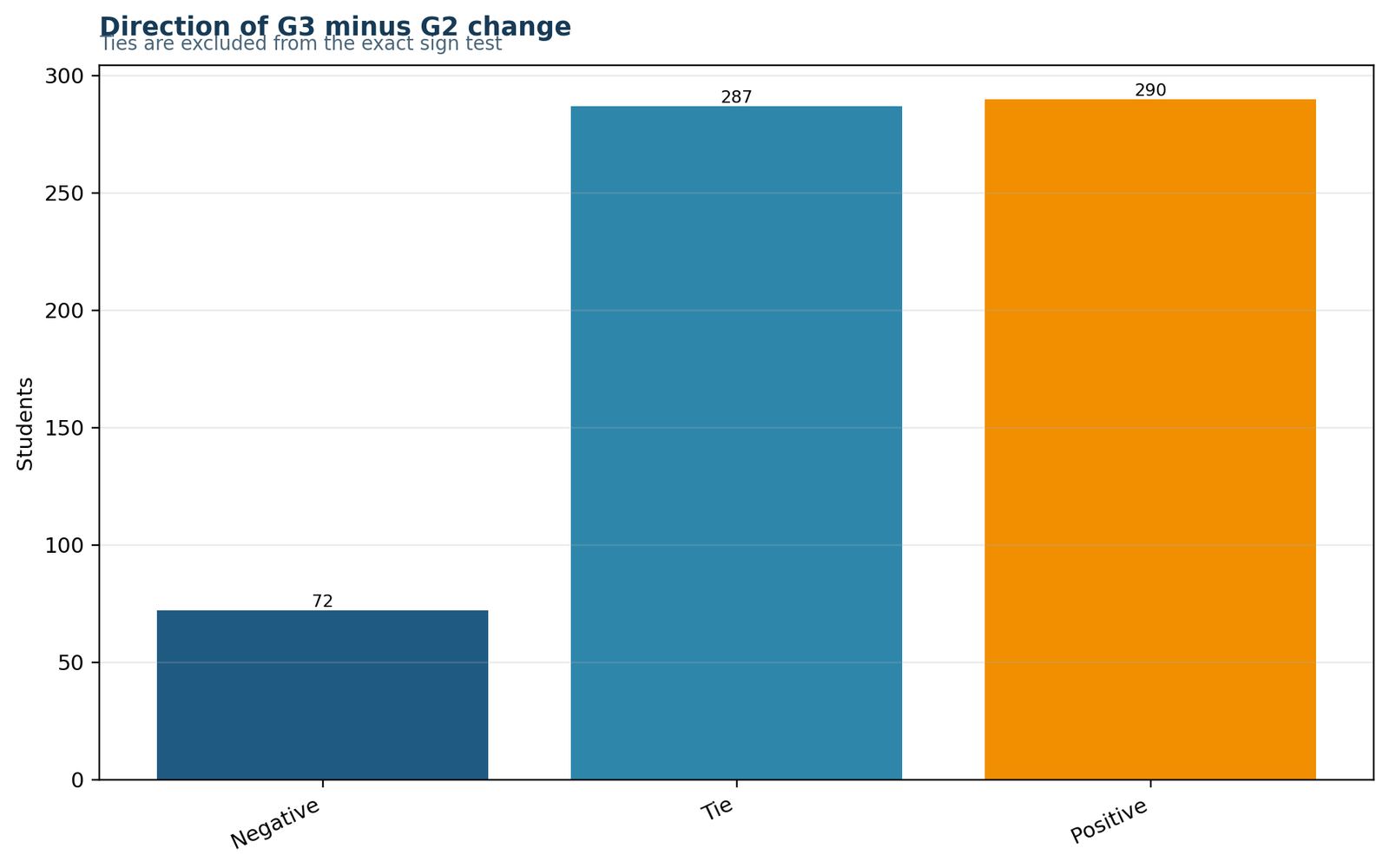
290 increases, 72 decreases and 287 ties are the complete directional decomposition of 649 pairs.
Among all records, 44.68% increased, 11.09% decreased and 44.22% were tied. The bar heights reconcile exactly to 649.
Interpretation checkpoint: The chart prevents the effective n=362 from being mistaken for the original sample size. Ties are not missing data; they are observed zero changes.
Difference Distribution: Direction Dominates Despite Asymmetric Extremes
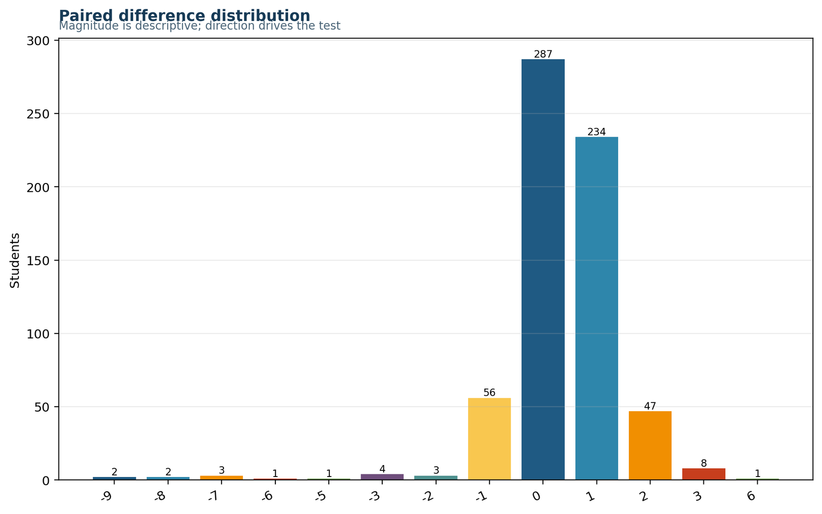
The distribution ranges from −9 to +6, with 287 zeros, 234 +1 changes and 56 −1 changes.
Most information lies near zero: 88.91% of pairs are tied or differ by one point. Large negative changes exist but are rare.
Interpretation checkpoint: The sign test intentionally prevents the two −9 and two −8 observations from dominating the inference; each contributes one negative sign.
Exact Null Distribution: Observed X = 290 Versus Expected 181
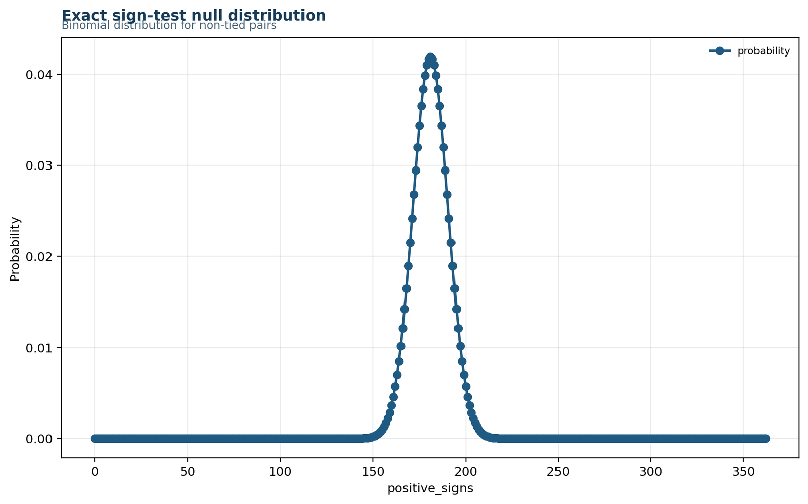
Under H0, X follows Binomial(362, 0.50), with mean 181 and standard deviation 9.513.
The observed count is 109 signs above the null mean, or 11.46 null standard deviations without continuity correction.
Interpretation checkpoint: The exact tail—not the normal approximation—is the reported analysis, producing p = 3.9796 × 10⁻³².
Two-Sided Region: Observed Count Far Beyond the Critical Boundary
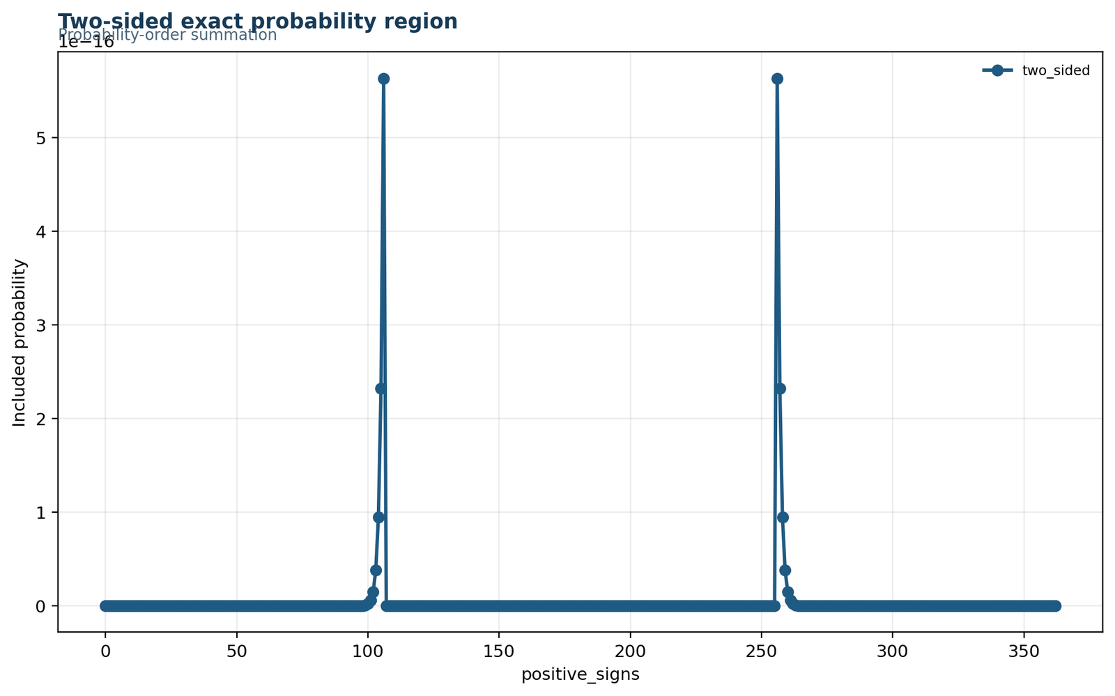
At a conservative exact α=.05, the rejection region is X≤161 or X≥201.
X=290 lies 89 counts beyond the upper critical boundary. The visual distance explains why rounding the p-value to .000 hides substantial information.
Interpretation checkpoint: Report the scientific-notation probability or p<.001, never p=0.
Sign Proportions: 80.11% Positive Among Changed Pairs
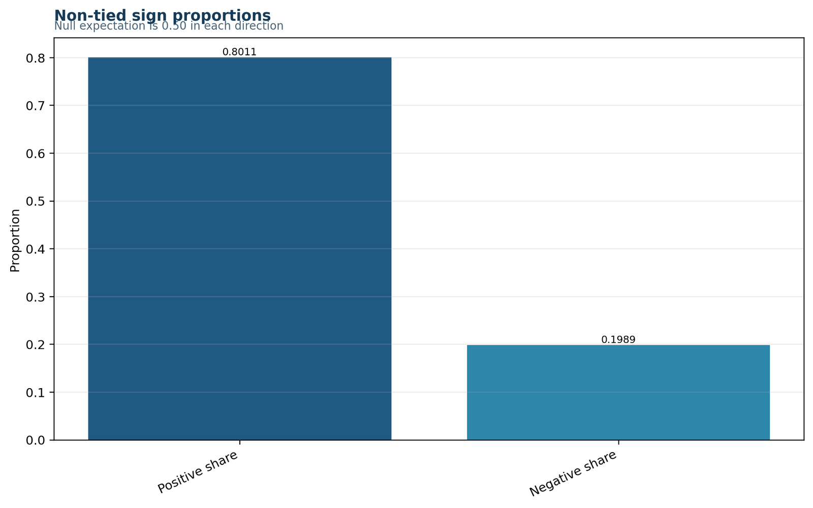
The non-tied positive proportion is 0.801105 and the negative proportion is 0.198895.
The exact 95% interval for the positive probability is 0.756208 to 0.840997, wholly above 0.50.
Interpretation checkpoint: The net directional advantage is 0.602210, and the directional odds are 4.0278 increases per decrease.
Result Summary: Strong Directional Evidence With a Zero Sample Median
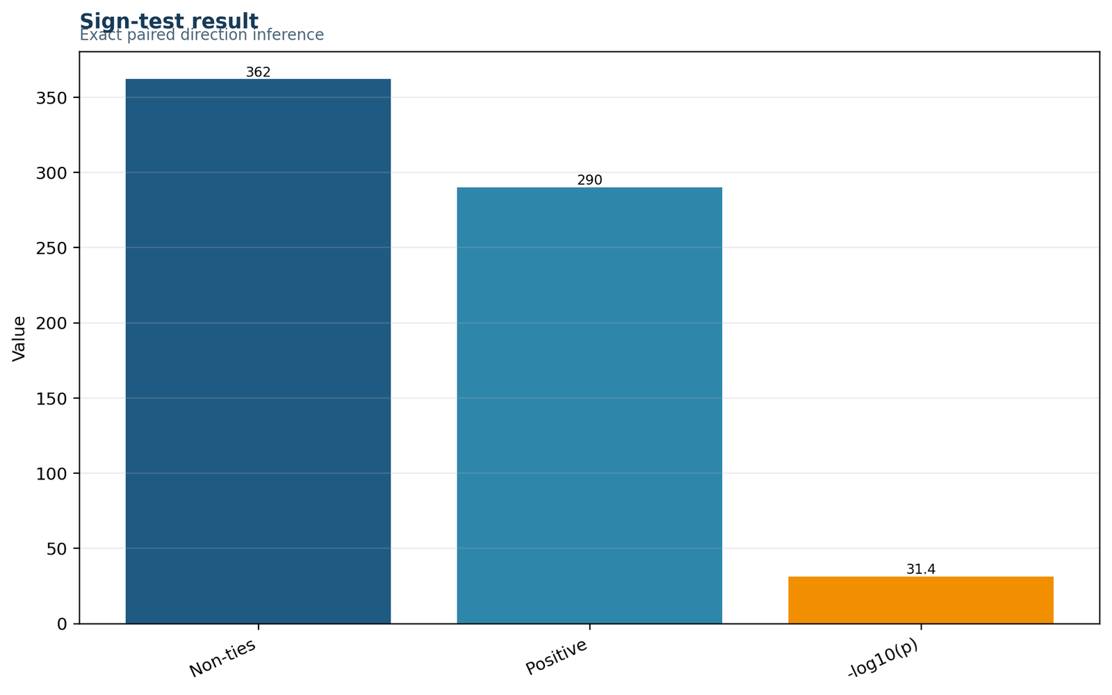
The summary combines X=290, n*=362, exact p≈3.98×10⁻³² and the reject decision.
The sample median difference is 0 because of 287 ties, while the median among nonzero differences is +1.
Interpretation checkpoint: The correct report emphasizes the conditional direction among changed pairs and retains the zero-median nuance.
R Sign Test Charts in Paired Rows
R chart pair 1: Change directions and Difference distribution
Direction counts
The R direction chart reproduces 290 positive, 72 negative and 287 tied pairs. It verifies that the R workflow uses the same subtraction order and tie definition as the workbook.
Difference distribution
The R distribution chart confirms the modal difference is 0 and the most common nonzero difference is +1. The rare long negative tail is descriptive rather than a weighted component of the sign statistic.
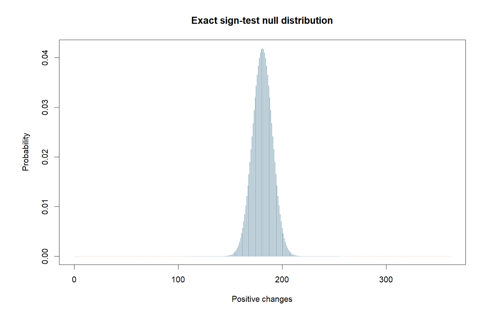
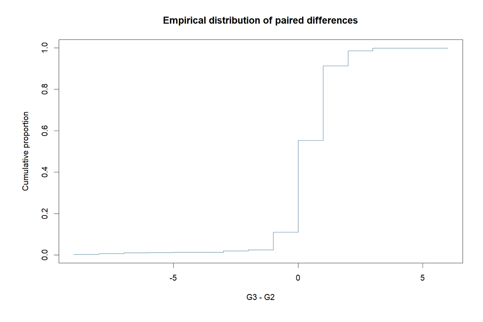
R chart pair 2: Exact binomial null and Cumulative paired difference
Exact null
The exact-null figure places X=290 against Binomial(362,.5). The observed count is visually detached from the probability mass centred at 181.
Cumulative difference
The cumulative sequence ends at +218 grade points, reaches a maximum of +241 near pair 621 and has a minimum of −1. This order-dependent curve is descriptive and must not be confused with the order-free sign test.
R chart pair 3: Non-tie balance and Result summary
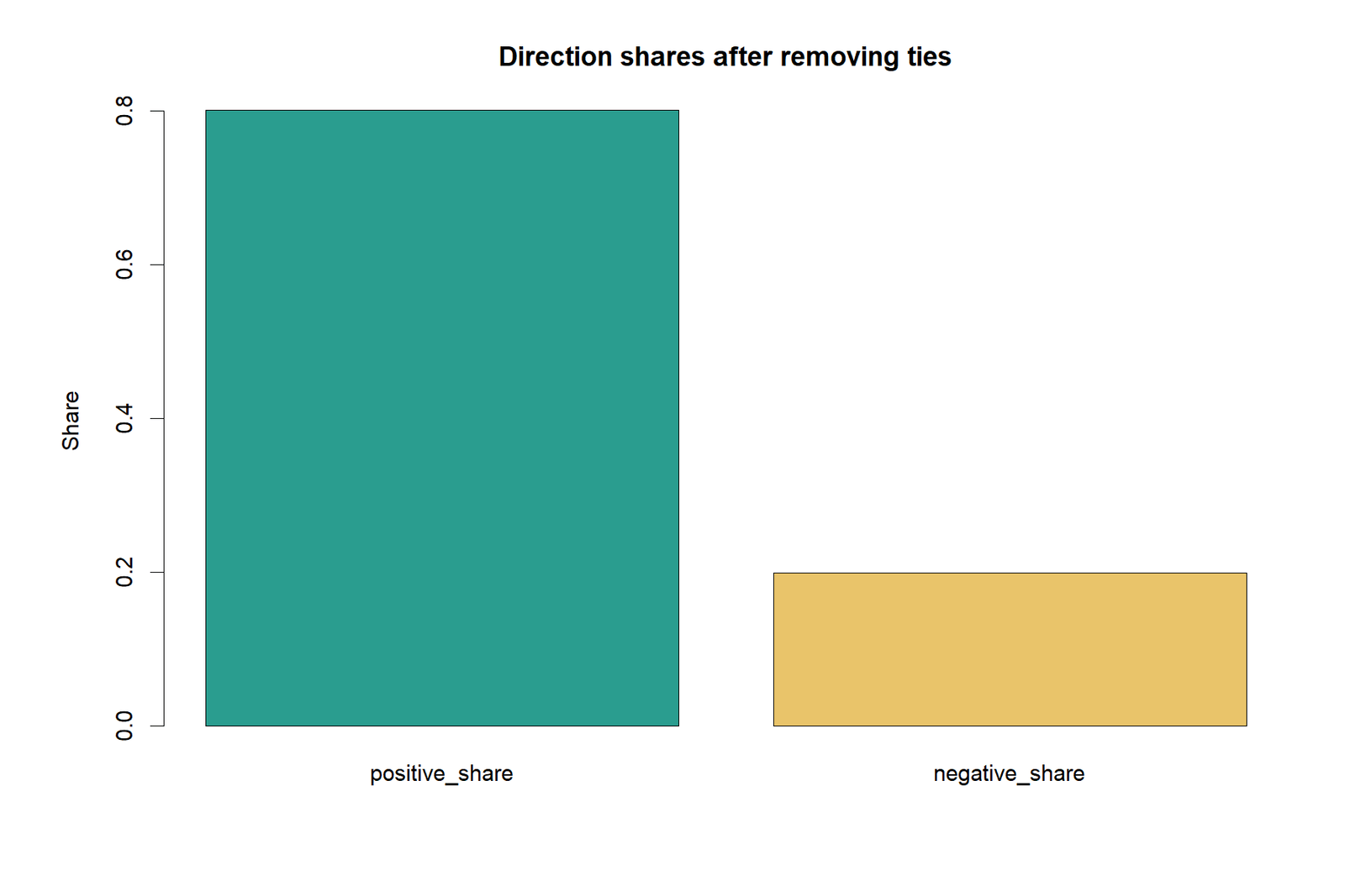
Non-tie balance
The non-tie chart removes 287 zeros and displays the 80.11% versus 19.89% direction split used in the exact test.
Result summary
The final R panel reconciles counts, exact probability and decision. Agreement with Python and Excel confirms that the analysis is not software-specific.
Sign Test in Python, R, SPSS and Excel
Python
- Create d = G3 − G2.
- Count d>0, d<0 and d=0.
- Use
scipy.stats.binomtest(290, 362, .5). - Request the exact confidence interval for the positive-sign probability.
R
- Compute
d <- G3 - G2. - Set
x <- sum(d > 0). - Set
n <- sum(d != 0). - Run
binom.test(x, n, p=.5).
SPSS
- Keep G2 and G3 as paired variables.
- Use the paired Sign procedure under Nonparametric Tests.
- Verify positive, negative and tie counts.
- Report SPSS .000 as p<.001, not p=0.
Excel
- Calculate row differences.
- Use COUNTIF for the three direction categories.
- Use BINOM.DIST on the smaller tail.
- Format tiny probabilities in scientific notation.
Cross-Software Reconciliation
| Output | Python | R | SPSS display | Excel/verified |
|---|---|---|---|---|
| Positive | 290 | 290 | 290 | 290 |
| Negative | 72 | 72 | 72 | 72 |
| Ties | 287 | 287 | 287 | 287 |
| Non-ties | 362 | 362 | 362 | 362 |
| Two-sided p | 3.9795987705E−32 | 3.9795987705E−32 | .000 | 3.9795987705E−32 |
| Decision | Reject H0 | Reject H0 | Reject H0 | Reject H0 |
Software agreement depends on matching the same alternative and tie convention. Some packages label the procedure as a median test, while others expose the binomial calculation directly. The counts and null probability are the common core.
Expandable Sign Test Code
Python: exact paired sign test
import numpy as np
from scipy.stats import binomtest

g2 = np.asarray(g2_values, dtype=float)
g3 = np.asarray(g3_values, dtype=float)

if g2.shape != g3.shape:
    raise ValueError("G2 and G3 must have the same number of paired values.")

d = g3 - g2
positive = int(np.sum(d > 0))
negative = int(np.sum(d < 0))
ties = int(np.sum(d == 0))
non_ties = positive + negative

result = binomtest(
    k=positive,
    n=non_ties,
    p=0.5,
    alternative="two-sided"
)
ci = result.proportion_ci(confidence_level=0.95, method="exact")

print({
    "positive": positive,
    "negative": negative,
    "ties": ties,
    "non_ties": non_ties,
    "p_value": result.pvalue,
    "positive_probability_ci": (ci.low, ci.high),
})
R: exact paired sign test
d <- G3 - G2

positive <- sum(d > 0, na.rm = TRUE)
negative <- sum(d < 0, na.rm = TRUE)
ties <- sum(d == 0, na.rm = TRUE)
non_ties <- positive + negative

fit <- binom.test(
  x = positive,
  n = non_ties,
  p = 0.5,
  alternative = "two.sided",
  conf.level = 0.95
)

list(
  positive = positive,
  negative = negative,
  ties = ties,
  non_ties = non_ties,
  p_value = fit$p.value,
  confidence_interval = fit$conf.int
)
SPSS: paired sign test syntax
NPAR TESTS
  /SIGN = G3 WITH G2 (PAIRED)
  /MISSING ANALYSIS.
Check that the output direction matches G3 minus G2. If the variable order is reversed, positive and negative labels reverse while the two-sided probability remains unchanged.
Excel: transparent formulas
C5: =B5-A5
Positive: =COUNTIF(C5:C653,">0")
Negative: =COUNTIF(C5:C653,"<0")
Ties: =COUNTIF(C5:C653,0)
NonTies: =Positive+Negative
TwoSidedP: =2*BINOM.DIST(MIN(Positive,Negative),NonTies,0.5,TRUE)
One-sample sign test adaptation
# Compare observations x with hypothesised median m0
d = x - m0
positive = sum(d > 0)
negative = sum(d < 0)
result = binomtest(positive, positive + negative, p=0.5)
One-sided positive-change alternative
# Python
binomtest(290, 362, p=0.5, alternative="greater")

# R
binom.test(290, 362, p=0.5, alternative="greater")
The one-sided exact p-value is 1.9897993853 × 10⁻³². A one-sided alternative must be prespecified rather than selected after observing 290 positive signs.
How to Interpret and Report the Sign Test
APA-Style Worked Report
An exact two-sided paired sign test examined the direction of change from second-period grade (G2) to final grade (G3) for 649 students. There were 290 positive differences, 72 negative differences and 287 ties, leaving 362 non-tied pairs for the exact binomial test. Positive changes constituted 80.11% of non-tied pairs, 95% exact CI [75.62%, 84.10%]. The direction distribution differed significantly from equal positive and negative probabilities, exact p < .001. Thus, among students whose grade changed, increases were substantially more common than decreases.
Reporting Table
| Item | Report |
|---|---|
| Design | Paired exact sign test |
| Difference definition | G3 − G2 |
| Positive / negative / ties | 290 / 72 / 287 |
| Effective n | 362 non-tied pairs |
| Positive proportion | 0.8011 |
| Exact 95% CI | [0.7562, 0.8410] |
| Exact two-sided p | 3.9796 × 10⁻³²; report p<.001 |
| Observed median difference | 0 |
| Interpretive scope | Directional imbalance among non-tied pairs |
Significant Two-Sided Result
Significant
An exact paired sign test compared later measure with earlier measure.
There were X positive, Y negative and T tied differences.
The positive-sign proportion was p̂, exact 95% CI [lower, upper], exact p value.
Non-Significant Result
Not significant
The observed positive and negative directions did not provide sufficient evidence against equal sign probabilities, exact p = value.
The exact confidence interval for the positive-sign probability was [lower, upper].
Prespecified One-Sided Result
Directional
A prespecified one-sided sign test evaluated whether positive changes were more likely than negative changes.
Positive changes occurred in X of n* non-tied pairs, exact one-sided p value.
Common Sign Test Mistakes and Corrections
| Mistake | Why it is wrong | Correction |
|---|---|---|
| Using 649 as the binomial n | Ties do not contribute positive or negative signs. | Use n*=290+72=362 and report 287 ties separately. |
| Reporting p=0 | The exact probability is tiny but positive. | Report p<.001 or 3.9796×10⁻³². |
| Claiming the sample median difference is positive | The observed median difference is exactly 0. | Describe the positive imbalance among non-tied pairs. |
| Reversing the subtraction silently | It changes which direction is labelled positive. | State d=G3−G2 before analysis. |
| Calling the test Wilcoxon | The sign test does not rank magnitudes. | Name the exact paired sign test. |
| Ignoring pairing | Independent-sample analysis discards within-student matching. | Compute one difference per student. |
| Deleting ties as missing data | A tie is an observed outcome, not missingness. | Show the tie count and percentage. |
| Using a one-sided p after seeing the data | That inflates selective-inference risk. | Prespecify the directional alternative. |
| Interpreting association as causation | The test does not identify a cause of change. | Limit conclusions to observed directional evidence. |
| Focusing only on significance | A huge sample can produce small p-values. | Report 80.11%, its interval, ties and direction odds. |
Quality-Control Checklist
Sign Test Practice Questions With Solutions
1. Recalculate the effective sample size
A paired study has 41 positive changes, 19 negative changes and 20 ties. What is n*?
2. Choose the correct tail
A protocol specified before data collection that the later score would be higher. Which alternative should be used?
3. Interpret a zero median with many ties
Suppose the sample median difference is zero, but 90 of 110 non-tied pairs are positive. Is a sign test meaningful?
4. Distinguish sign test from paired t test
Which method uses the actual sizes of the paired differences?
5. Interpret the current result
What does 290 positive versus 72 negative changes establish?
6. Check the current exact count
Under H0 with n*=362, what is the expected number of positive signs?
Sign Test Reports and Worked Files
The downloadable files reproduce the same G3 − G2 direction, counts and exact inference. Use the workbook to inspect every paired difference and formula.
Download Verification
| File | Expected core values |
|---|---|
| Python report | Positive 290; negative 72; ties 287; exact p 3.9795987705E−32 |
| R report | Same counts, exact binomial result and confidence interval |
| SPSS output | Paired Sign procedure; p displayed as .000 because of print precision |
| Excel workbook | 649 raw pairs, formulas, difference table, diagnostics and reporting audit |
Sign Test Frequently Asked Questions
What is a sign test?
A sign test is an exact or approximate nonparametric procedure that counts positive and negative deviations from a benchmark. In paired data, the deviations are within-pair differences.
What is the sign test formula?
After removing ties, let X be the number of positive signs and n* the number of non-ties. Under the usual null, X follows Binomial(n*,0.50).
Why are ties excluded?
A zero difference is neither positive nor negative, so it provides no direction. Ties must still be reported because they describe the data and reduce the effective sample size.
What were the worked counts?
The 649 pairs contained 290 increases, 72 decreases and 287 ties. The exact test therefore used n*=362.
What was the exact p-value?
The exact two-sided probability was 3.9795987705×10⁻³². In conventional reporting this is p<.001.
Can the median difference be zero when the sign test is significant?
Yes. Here 287 ties force the observed median difference to zero, while 290 of 362 non-tied differences are positive. The test detects conditional directional imbalance.
Is the sign test the same as Wilcoxon signed-rank?
No. The sign test uses only direction. Wilcoxon signed-rank uses direction and ranked absolute differences.
Does the sign test require normality?
No. Its exact null distribution is binomial.
Does the sign test require symmetry?
No. Symmetry is not required because magnitudes are discarded.
What does the positive-sign confidence interval mean?
The exact 95% interval of 0.7562 to 0.8410 estimates the probability that a changed pair is positive, conditional on the difference being nonzero.
Can Excel perform a sign test?
Yes. Use formulas to count positive, negative and tied differences, then calculate the exact binomial tail with BINOM.DIST.
How should SPSS .000 be reported?
Report p<.001, not p=.000 and not p=0.
Sign Test Conclusion
The exact paired sign test provides a clear directional result for the 649 G2–G3 pairs. Of the 362 students whose grade changed, 290 increased and 72 decreased. The positive-sign proportion was 0.8011, with an exact 95% confidence interval from 0.7562 to 0.8410, and the two-sided exact probability was approximately 3.98 × 10⁻³².
The strongest interpretation is also the most precise: among changed pairs, grade increases were far more common than decreases. The analysis does not require normality or symmetry, does not allow rare extreme magnitudes to dominate, and does not conceal the 287 ties. Because those ties make the observed median difference equal to zero, a high-quality report should describe the directional imbalance rather than claiming a positive observed median.
The worked Python, R, SPSS and Excel files all reconcile to the same counts and decision. Readers can use the formulas, code and reporting templates above to reproduce the sign test for paired data or adapt it to a one-sample median benchmark.

