
Post Hoc Analysis, Multiple Comparisons, Adjusted p-values and Familywise Error Control
Bonferroni Correction: Formula, Interpretation, SPSS, Python, R and Excel Guide
Bonferroni Correction is a simple and conservative method for controlling familywise error when several pairwise comparisons are tested after ANOVA. In this worked Salar Cafe example, G3 final grade is compared across four studytime groups. The one-way ANOVA is significant, and the Bonferroni post hoc test shows that four of the six pairwise comparisons remain significant after correction.
Quick Answer: Bonferroni Correction Result
The Bonferroni Correction was applied after a significant one-way ANOVA comparing G3 final grade across four studytime groups. Because there are four groups, there are 6 pairwise comparisons. With a familywise alpha of .05, the Bonferroni per-comparison alpha is .008333.
The one-way ANOVA result was significant, F(3, 645) = 15.876, p = 5.705728e-10. The Bonferroni-adjusted pairwise results show that studytime 1 differs from studytime 2, studytime 1 differs from studytime 3, studytime 1 differs from studytime 4, and studytime 2 differs from studytime 3. The comparisons studytime 2 vs 4 and studytime 3 vs 4 are not significant after Bonferroni correction.
Final interpretation: Bonferroni correction confirms that lower studytime is associated with lower mean G3. Studytime group 1 is significantly lower than groups 2, 3 and 4, and group 2 is significantly lower than group 3. Groups 2 and 4 do not differ significantly after correction, and groups 3 and 4 also do not differ significantly after correction.
Important reporting point: Bonferroni correction protects against false positives when many pairwise tests are run, but it can be conservative. A non-significant Bonferroni result does not always prove that two groups are identical; it means the difference was not strong enough after the multiple-comparison adjustment.
Table of Contents
- What Is Bonferroni Correction?
- Bonferroni Correction Formula
- Why Bonferroni Correction Is Needed After ANOVA
- Bonferroni Post Hoc Hypotheses
- Dataset and Variables Used
- Assumptions Before Bonferroni Post Hoc Testing
- SPSS Output Interpretation
- Python Chart-by-Chart Interpretation
- R Chart-by-Chart Validation
- SPSS, R, Python and Excel Workflows
- Code Blocks for Bonferroni Correction
- APA Reporting Wording
- Common Mistakes
- When to Use Bonferroni Correction
- Downloads and Resources
- Related Guides
- FAQs
What Is Bonferroni Correction?
Bonferroni Correction is a multiple-comparison adjustment used when a researcher tests several hypotheses in the same family of comparisons. In post hoc ANOVA analysis, this usually means comparing every pair of group means after the overall ANOVA has shown that at least one group mean differs.
The problem is simple. If you run one test at α = .05, the chance of a false positive is controlled at about 5% for that test. But if you run many tests, the chance of getting at least one false positive increases. Bonferroni correction solves this by making each individual comparison harder to call significant.
In this example, there are four studytime groups, so there are six pairwise comparisons. Bonferroni correction either divides the familywise alpha by the number of comparisons or multiplies each raw p-value by the number of comparisons. Both views lead to the same decision logic.
Simple definition: Bonferroni Correction is a post hoc p-value adjustment that controls familywise error by making pairwise comparisons more conservative.
This guide connects naturally with One Way ANOVA, Factorial ANOVA, ANOVA Assumptions, ANOVA in SPSS, ANOVA in R, ANOVA in Python, P Value, Null and Alternative Hypothesis, Type I and Type II Error and Statistical Power.
Bonferroni Correction Formula
The Bonferroni correction can be written in two common ways. The first method divides the familywise alpha by the number of comparisons:
Here, m is the number of pairwise comparisons. In this example, there are four groups, so the number of comparisons is:
With familywise α = .05:
The second method adjusts each p-value directly:
SPSS, Python and R commonly report Bonferroni-adjusted p-values. A pairwise comparison is significant when the adjusted p-value is below .05.
| Item | Value in This Example | Meaning |
|---|---|---|
| Number of groups | 4 | Studytime groups 1, 2, 3 and 4. |
| Number of pairwise comparisons | 6 | All possible group pairs. |
| Familywise alpha | .05 | Maximum error rate for the family of tests. |
| Bonferroni per-comparison alpha | .008333 | Corrected alpha when using the divided-alpha method. |
| Decision with adjusted p-values | padjusted < .05 | Significant after Bonferroni correction. |
Why Bonferroni Correction Is Needed After ANOVA
A one-way ANOVA tells whether at least one group mean differs from the others. It does not tell exactly which groups differ. After a significant ANOVA, a post hoc test is used to compare group pairs. When many pairwise comparisons are made, the false-positive risk increases, so a correction is needed.
In this example, the ANOVA result is significant, but the meaningful reporting question is more specific: which studytime groups have different mean G3 scores? Bonferroni correction answers that question while controlling the familywise error rate.
| Stage | Question | Result in This Example |
|---|---|---|
| One-way ANOVA | Do any studytime groups differ in mean G3? | Yes. F(3,645) = 15.876, p = 5.706e-10. |
| Bonferroni post hoc | Which studytime pairs differ after correction? | 1–2, 1–3, 1–4 and 2–3 are significant. |
| Interpretation | Where is the practical mean difference? | Lower studytime groups have lower mean G3, especially studytime 1. |
For broader mean-comparison context, review T Test vs ANOVA, Student’s T Test, Two Sample T Test, One Tailed T Test, Two Tailed T Test, T Test in SPSS, T Test in R and T Test in Python.
Bonferroni Post Hoc Hypotheses
Bonferroni post hoc analysis tests pairwise hypotheses. Each pair has its own null and alternative hypothesis, but the p-values are adjusted so the family of tests is controlled.
| Comparison | Null Hypothesis | Alternative Hypothesis | Bonferroni Decision |
|---|---|---|---|
| 1 vs 2 | μ1 = μ2 | μ1 ≠ μ2 | Significant after correction. |
| 1 vs 3 | μ1 = μ3 | μ1 ≠ μ3 | Significant after correction. |
| 1 vs 4 | μ1 = μ4 | μ1 ≠ μ4 | Significant after correction. |
| 2 vs 3 | μ2 = μ3 | μ2 ≠ μ3 | Significant after correction. |
| 2 vs 4 | μ2 = μ4 | μ2 ≠ μ4 | Not significant after correction. |
| 3 vs 4 | μ3 = μ4 | μ3 ≠ μ4 | Not significant after correction. |
Decision for this example: Four pairwise differences remain significant after Bonferroni correction. Studytime group 1 is significantly lower than every other group, and studytime group 2 is significantly lower than studytime group 3. The evidence does not support a corrected difference between groups 2 and 4 or between groups 3 and 4.
Dataset and Variables Used
The worked example uses student performance data. The dependent variable is G3 final grade. The post hoc factor is studytime, which has four groups. The analysis uses 649 valid cases.
| Variable | Role | Levels / Type | Why It Matters |
|---|---|---|---|
| G3 | Dependent variable | Numeric final grade | The outcome whose group means are compared. |
| studytime | Post hoc factor | 1, 2, 3, 4 | Defines the four groups used for ANOVA and Bonferroni pairwise comparisons. |
Group Descriptive Statistics
| Studytime Group | N | Mean G3 | SD | Variance | Minimum | Maximum | Interpretation |
|---|---|---|---|---|---|---|---|
| 1 | 212 | 10.8443 | 3.2186 | 10.3595 | 0 | 18 | Lowest mean G3. |
| 2 | 305 | 12.0918 | 3.2431 | 10.5179 | 0 | 19 | Higher than group 1. |
| 3 | 97 | 13.2268 | 2.5021 | 6.2605 | 8 | 18 | Highest mean G3. |
| 4 | 35 | 13.0571 | 3.0384 | 9.2319 | 6 | 19 | High mean but smallest sample size. |
| Total | 649 | 11.9060 | 3.2307 | 10.4370 | 0 | 19 | Overall final-grade distribution. |
The descriptive pattern explains why post hoc testing is useful. The mean rises from studytime 1 to studytime 3, while studytime 4 remains high but has fewer students. Bonferroni correction then identifies which of these visible mean differences remain statistically significant after controlling for multiple testing.
For supporting concepts, review Descriptive Statistics, Mean Median and Mode, Standard Deviation, Variance, Standard Error, Confidence Interval, Five Number Summary and Box Plot Interpretation.
Assumptions Before Bonferroni Post Hoc Testing
Bonferroni Correction adjusts for multiple comparisons, but it does not fix a poor ANOVA design. The same basic assumptions of one-way ANOVA should be considered before interpreting Bonferroni post hoc results.
| Assumption | Meaning | How This Example Handles It |
|---|---|---|
| Continuous outcome | The dependent variable should be numeric. | G3 is a numeric final-grade variable. |
| Categorical factor | The grouping variable should define independent groups. | Studytime defines four groups. |
| Independent observations | Each case should contribute one independent score. | Each student contributes one G3 value. |
| Overall ANOVA significance | Post hoc tests usually follow a significant omnibus test. | The ANOVA p-value is 5.705728e-10. |
| Homogeneity of variance | Group variances should be reasonably similar for standard ANOVA post hoc tests. | Levene based on mean is p = .400, so equality of variance is not rejected. |
| Reasonable distribution shape | Strong non-normality can affect inference, especially in small groups. | Histograms and Q-Q plots are used for distribution context. |
For assumption support, use ANOVA Assumptions, Levene Test, Bartlett’s Test, Brown-Forsythe Test, Hartley F Max Test, Cochran C Test, Q-Q Plot Normality Check, P-P Plot Normality Check, Shapiro-Wilk Test and Outlier Detection.
SPSS Output Interpretation for Bonferroni Correction
The SPSS output uses ONEWAY G3 BY studytime with descriptive statistics, homogeneity testing, ANOVA and Bonferroni post hoc comparisons. The key table is the Multiple Comparisons table under Bonferroni.
SPSS Reading Order
| SPSS Output Area | What to Read | Why It Matters |
|---|---|---|
| Case Processing Summary | 649 included, 0 excluded | Confirms all valid cases were used. |
| Descriptives | N, mean, SD and confidence interval | Shows group mean pattern before testing pairs. |
| Test of Homogeneity | Levene based on mean p = .400 | Supports the equal-variance context for standard ANOVA post hoc testing. |
| ANOVA table | F(3,645) = 15.876, p < .001 | Shows that post hoc testing is justified. |
| Bonferroni Multiple Comparisons | Mean difference, SE, adjusted Sig. and CI | Main pairwise decision table. |
SPSS One-Way ANOVA Table
| Source | Sum of Squares | df | Mean Square | F | Sig. | Interpretation |
|---|---|---|---|---|---|---|
| Between groups | 465.078 | 3 | 155.026 | 15.876 | < .001 | At least one studytime group mean differs. |
| Within groups | 6298.189 | 645 | 9.765 | Residual variation within studytime groups. | ||
| Total | 6763.267 | 648 | Total G3 variation. |
SPSS Bonferroni Multiple Comparisons
| Comparison | Mean Difference | Std. Error | Bonferroni Sig. | 95% CI | Decision |
|---|---|---|---|---|---|
| 1 vs 2 | -1.247 | .279 | < .001 | -1.99 to -.51 | Significant. |
| 1 vs 3 | -2.382 | .383 | < .001 | -3.40 to -1.37 | Significant. |
| 1 vs 4 | -2.213 | .570 | .001 | -3.72 to -.70 | Significant. |
| 2 vs 3 | -1.135 | .364 | .011 | -2.10 to -.17 | Significant. |
| 2 vs 4 | -.965 | .558 | .504 | -2.44 to .51 | Not significant. |
| 3 vs 4 | .170 | .616 | 1.000 | -1.46 to 1.80 | Not significant. |
SPSS interpretation summary: The omnibus one-way ANOVA is significant, so Bonferroni post hoc comparisons are interpreted. Studytime group 1 differs significantly from groups 2, 3 and 4. Studytime group 2 also differs significantly from group 3. The 2 vs 4 and 3 vs 4 comparisons are not significant after Bonferroni correction.
Python Chart-by-Chart Interpretation
The Python chart sequence explains Bonferroni Correction through group distributions, group means, adjusted p-values, mean differences with Bonferroni confidence intervals and group sample sizes.
Python Chart 1: Group Distributions by Studytime
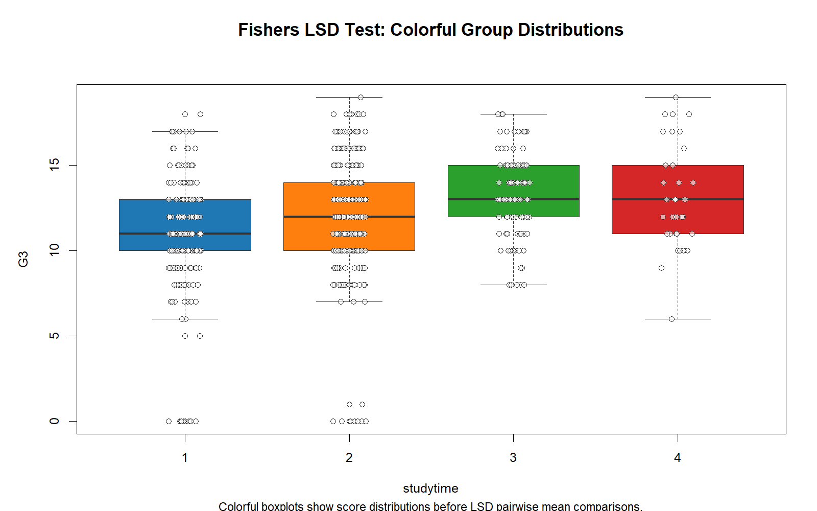
The first chart shows how G3 final grade is distributed within each studytime group. Studytime group 1 has the lowest central pattern, while studytime groups 3 and 4 sit higher on the grade scale. The visible group separation explains why the one-way ANOVA becomes significant.
The boxplot also shows that the groups are not identical in spread or sample behavior. Bonferroni correction does not remove the need to inspect distributions; it controls the multiple-testing error after the ANOVA and pairwise comparisons are run.
Python Chart 2: Group Means with Confidence Intervals
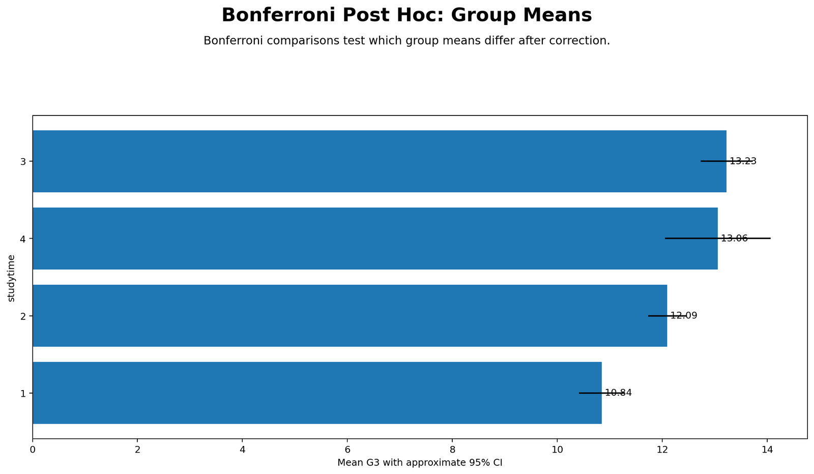
The group mean chart shows a clear increase from studytime 1 to studytime 3. Group 4 remains high, but it has the smallest sample size, which makes its interval wider than the larger groups.
This visual supports the post hoc result. The largest corrected differences involve group 1 compared with higher studytime groups, especially group 3.
Python Chart 3: Bonferroni-Adjusted p-values
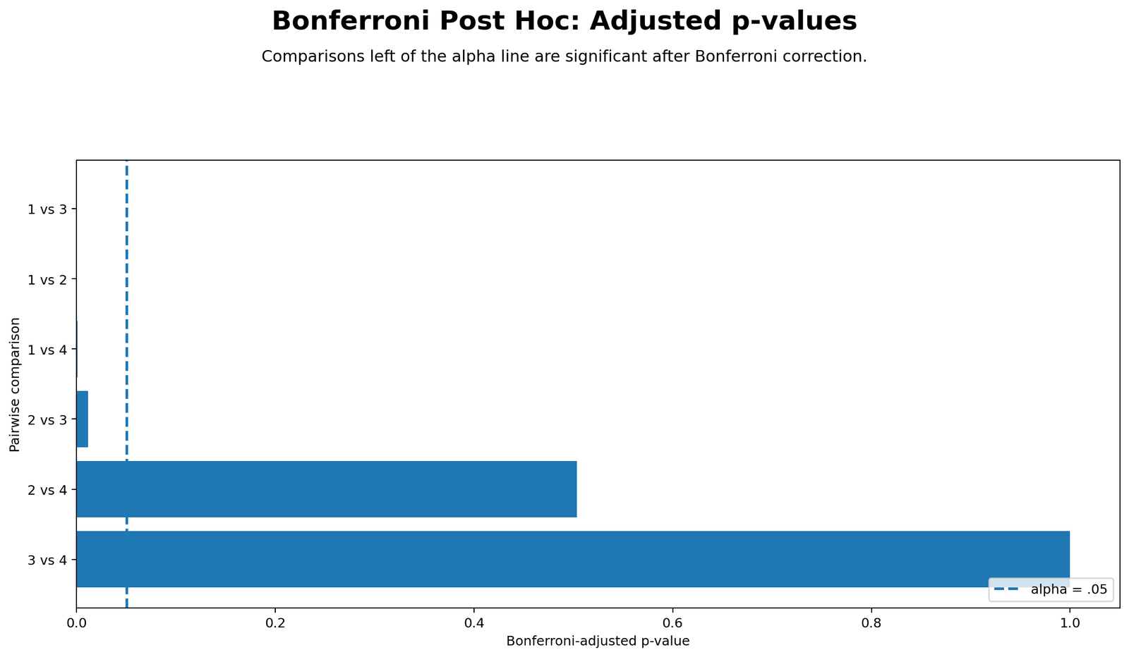
The adjusted p-value chart places each comparison against the α = .05 decision line. The comparisons 1 vs 3, 1 vs 2, 1 vs 4 and 2 vs 3 fall on the significant side after Bonferroni correction.
The comparisons 2 vs 4 and 3 vs 4 remain to the right of the alpha line and are not significant after correction. This means the highest studytime groups are not all statistically separated from each other after familywise error control.
Python Chart 4: Bonferroni Mean Differences with Confidence Intervals
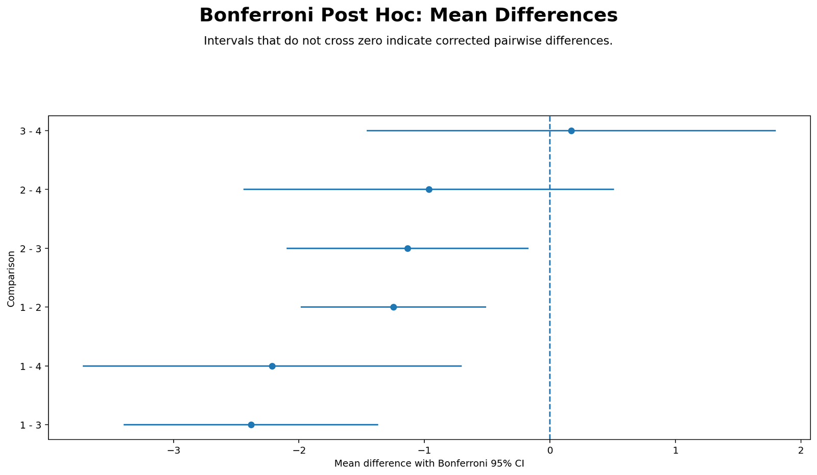
The mean-difference chart shows which corrected intervals cross zero. Comparisons whose intervals do not cross zero are significant after Bonferroni correction. The differences involving group 1 and the comparison 2 vs 3 do not cross zero.
The intervals for 2 vs 4 and 3 vs 4 cross zero. This matches the adjusted p-value result and confirms that those two comparisons should be reported as not significant after correction.
Python Chart 5: Group Sample Sizes
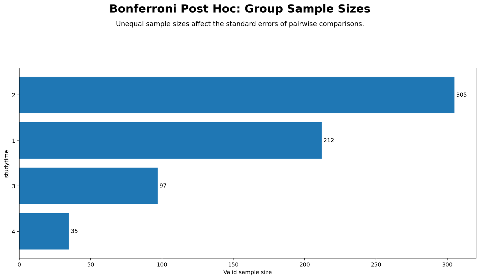
The sample-size chart shows that the groups are unequal: group 2 has 305 cases, group 1 has 212, group 3 has 97 and group 4 has 35. This matters because smaller groups usually have larger standard errors in pairwise comparisons.
Group 4 has a high mean but only 35 cases. That smaller sample size helps explain why some comparisons involving group 4 are less precise and why the 2 vs 4 comparison does not remain significant after correction.
R Chart-by-Chart Validation
The R charts validate the same Bonferroni Correction workflow using a second software environment. The R results confirm the same group distribution, mean pattern, adjusted p-value decision, confidence interval interpretation and sample-size context.
R Chart 1: Group Distributions by Studytime
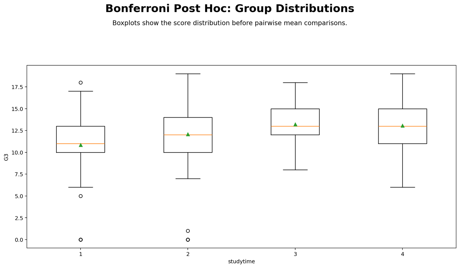
The R distribution chart confirms the same pattern shown by Python. Studytime group 1 has a lower grade distribution, while groups 3 and 4 appear higher.
This validates the descriptive foundation for the post hoc test. The statistical comparisons are not floating numbers; they are attached to a visible group pattern.
R Chart 2: Group Means with Confidence Intervals
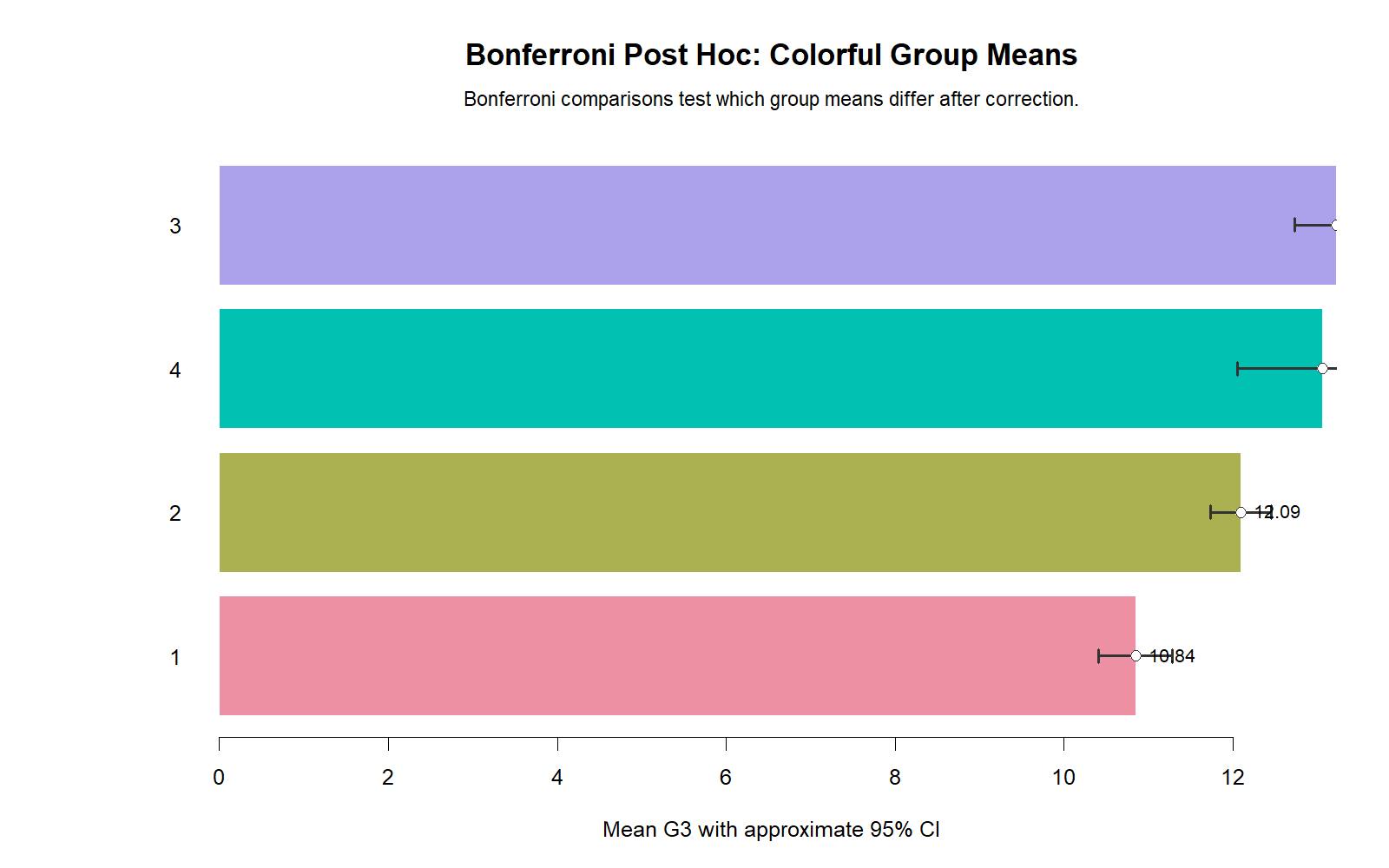
The R mean chart confirms that studytime group 1 has the lowest mean and group 3 has the highest mean. Group 4 remains close to group 3 but with a wider interval because its sample size is smaller.
This supports the final interpretation that the strongest differences involve lower studytime compared with higher studytime groups.
R Chart 3: Bonferroni-Adjusted p-values
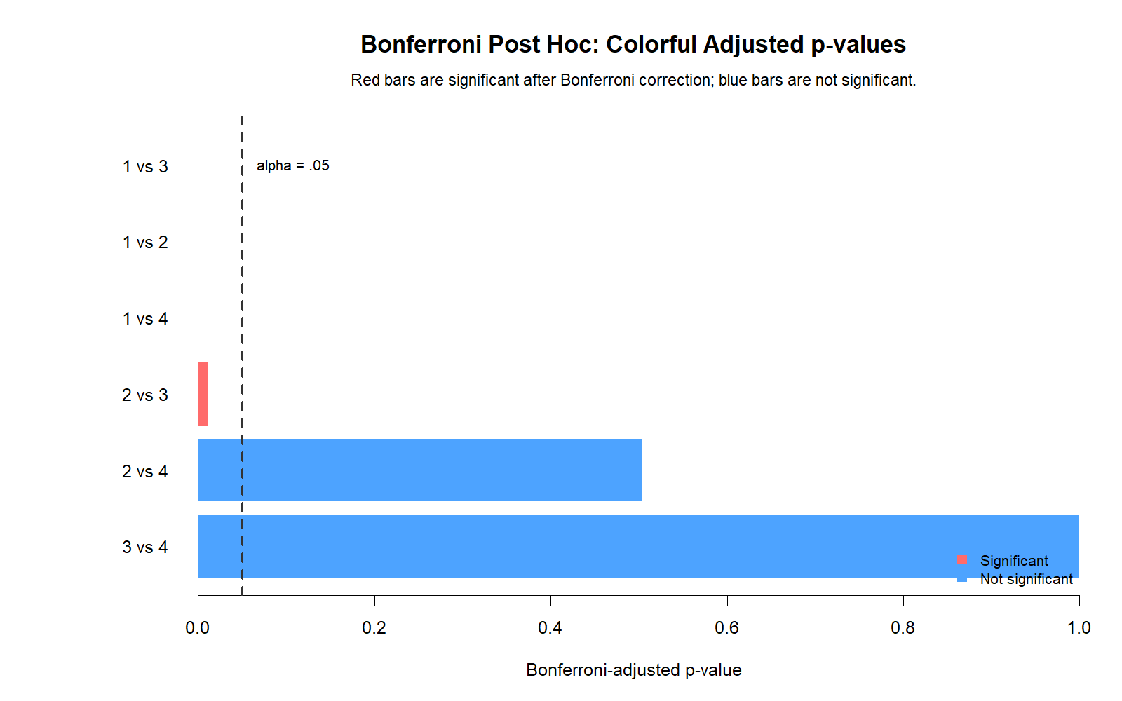
The R adjusted p-value chart confirms the Python decision pattern. The comparisons 1 vs 2, 1 vs 3, 1 vs 4 and 2 vs 3 are significant after correction.
The comparisons 2 vs 4 and 3 vs 4 are not significant after correction. This repeated result across R, Python and SPSS makes the post hoc conclusion stable for reporting.
R Chart 4: Bonferroni Mean Differences with Confidence Intervals
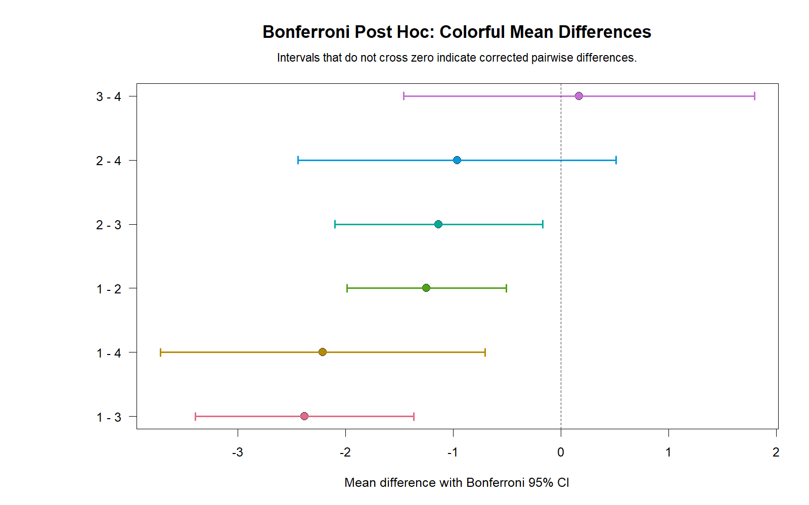
The R mean-difference chart confirms that the significant comparisons have intervals away from zero. The non-significant comparisons have intervals that cross zero.
This chart is useful because it gives both direction and uncertainty. A negative difference such as 1 vs 3 means group 1 has a lower mean than group 3.
R Chart 5: Group Sample Sizes
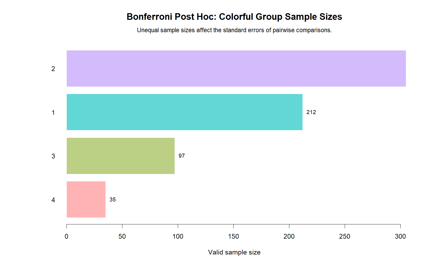
The R sample-size chart confirms the unequal group sizes. Group 2 is the largest group, and group 4 is the smallest group.
This context helps explain why group 4 comparisons need careful interpretation. Bonferroni correction controls the familywise error rate, while the sample-size chart explains the precision behind the pairwise estimates.
SPSS, R, Python and Excel Workflows for Bonferroni Correction
The same Bonferroni Correction workflow can be reproduced in SPSS, R, Python and Excel. SPSS provides Bonferroni directly in the One-Way ANOVA post hoc menu. R can use pairwise.t.test() with p.adjust.method = "bonferroni". Python can calculate adjusted p-values by multiplying raw p-values by the number of comparisons. Excel can support the calculation with formulas, but SPSS, R or Python is better for final reproducible reporting.
SPSS Workflow
| Step | SPSS Menu or Syntax | Purpose |
|---|---|---|
| Open dataset | File > Open > Data | Load G3 and studytime. |
| Run one-way ANOVA | Analyze > Compare Means > One-Way ANOVA | Set up group mean comparison. |
| Dependent variable | G3 | Outcome variable. |
| Factor | studytime | Grouping variable. |
| Options | Descriptive and Homogeneity | Request means and Levene test. |
| Post Hoc | Bonferroni | Request corrected pairwise comparisons. |
| Read output | Multiple Comparisons table | Interpret adjusted Sig. and confidence intervals. |
R Workflow
| Step | R Action | Purpose |
|---|---|---|
| Read data | read.csv("dataset.csv") | Load the dataset. |
| Convert group | factor(studytime) | Define studytime as categorical. |
| Run ANOVA | aov(G3 ~ studytime) | Test overall mean difference. |
| Run pairwise tests | pairwise.t.test(..., p.adjust.method="bonferroni") | Apply Bonferroni adjustment. |
| Summarize means | group_by(studytime) | Report group n, mean and SD. |
| Plot results | Boxplots, means, adjusted p-values and CIs | Explain the result visually. |
Python Workflow
| Step | Python Action | Purpose |
|---|---|---|
| Read data | pandas.read_csv() | Load G3 and studytime. |
| Run ANOVA | scipy.stats.f_oneway() or statsmodels | Confirm overall group difference. |
| Generate pairs | itertools.combinations(groups, 2) | Create all group pairs. |
| Run t-tests | scipy.stats.ttest_ind() | Calculate raw pairwise p-values. |
| Adjust p-values | min(raw_p * m, 1) | Apply Bonferroni correction. |
| Report | Adjusted p-values and confidence intervals | Present corrected pairwise decisions. |
Excel Workflow
| Excel Task | Formula or Tool | Purpose |
|---|---|---|
| Prepare data | Columns for G3 and studytime | Organize the dataset. |
| Group means | PivotTable average of G3 by studytime | Show descriptive pattern. |
| Group SD | =STDEV.S(range) | Calculate group spread. |
| Group N | =COUNT(range) | Calculate group sample size. |
| Number of comparisons | =k*(k-1)/2 | Calculate m. |
| Corrected alpha | =0.05/m | Apply divided-alpha Bonferroni rule. |
| Adjusted p-value | =MIN(raw_p*m,1) | Apply adjusted-p Bonferroni rule. |
Code Blocks for Bonferroni Correction
SPSS Syntax for Bonferroni Correction
* Bonferroni Correction post hoc test in SPSS.
* Dependent variable: G3.
* Factor: studytime.

TITLE "Bonferroni Correction Post Hoc Analysis".

ONEWAY G3 BY studytime
  /STATISTICS DESCRIPTIVES HOMOGENEITY
  /POSTHOC = BONFERRONI ALPHA(.05)
  /MISSING ANALYSIS.

EXAMINE VARIABLES=G3 BY studytime
  /PLOT BOXPLOT HISTOGRAM NPPLOT
  /COMPARE GROUPS
  /STATISTICS DESCRIPTIVES
  /CINTERVAL 95
  /MISSING LISTWISE
  /NOTOTAL.

OUTPUT EXPORT
  /CONTENTS EXPORT=VISIBLE
  /PDF DOCUMENTFILE="Bonferroni-Correction-SPSS-Output.pdf".
Python Code for Bonferroni Correction
import pandas as pd
import numpy as np
from itertools import combinations
from scipy import stats

df = pd.read_csv("dataset.csv")

df["G3"] = pd.to_numeric(df["G3"], errors="coerce")
df["studytime"] = df["studytime"].astype("category")

data = df[["G3", "studytime"]].dropna().copy()

# Group summary
summary = data.groupby("studytime")["G3"].agg(
    n="count",
    mean="mean",
    standard_deviation="std",
    variance="var",
    standard_error=lambda x: x.std(ddof=1) / np.sqrt(x.count()),
    minimum="min",
    maximum="max"
).reset_index()

print(summary)

# One-way ANOVA
groups = [
    group["G3"].to_numpy()
    for _, group in data.groupby("studytime", observed=True)
]

anova = stats.f_oneway(*groups)
print("ANOVA F:", anova.statistic)
print("ANOVA p:", anova.pvalue)

# Bonferroni pairwise comparisons
labels = sorted(data["studytime"].dropna().unique())
pairs = list(combinations(labels, 2))
m = len(pairs)

results = []

for g1, g2 in pairs:
    x1 = data.loc[data["studytime"] == g1, "G3"].to_numpy()
    x2 = data.loc[data["studytime"] == g2, "G3"].to_numpy()

    t_stat, raw_p = stats.ttest_ind(x1, x2, equal_var=True)
    adj_p = min(raw_p * m, 1.0)

    mean_diff = x1.mean() - x2.mean()

    results.append({
        "group_1": g1,
        "group_2": g2,
        "mean_group_1": x1.mean(),
        "mean_group_2": x2.mean(),
        "mean_difference_group_1_minus_group_2": mean_diff,
        "t_value": t_stat,
        "raw_p_value": raw_p,
        "bonferroni_adjusted_p_value": adj_p,
        "decision_alpha_0_05": "Significant after Bonferroni correction"
        if adj_p < 0.05 else "Not significant after Bonferroni correction"
    })

pairwise_table = pd.DataFrame(results)
print(pairwise_table)
R Code for Bonferroni Correction
# Bonferroni Correction post hoc analysis in R

library(tidyverse)
library(car)

df <- read.csv("dataset.csv")

df$G3 <- as.numeric(df$G3)
df$studytime <- as.factor(df$studytime)

data <- df %>%
  select(G3, studytime) %>%
  drop_na()

# Group summary
data %>%
  group_by(studytime) %>%
  summarise(
    n = n(),
    mean_G3 = mean(G3),
    sd_G3 = sd(G3),
    variance_G3 = var(G3),
    se_G3 = sd(G3) / sqrt(n()),
    minimum = min(G3),
    maximum = max(G3),
    .groups = "drop"
  )

# Assumption context
leveneTest(G3 ~ studytime, data = data)

# One-way ANOVA
anova_model <- aov(G3 ~ studytime, data = data)
summary(anova_model)

# Bonferroni pairwise comparisons
pairwise.t.test(
  x = data$G3,
  g = data$studytime,
  p.adjust.method = "bonferroni",
  pool.sd = TRUE
)

# Optional: Tukey-style table with Bonferroni-adjusted p-values
pairwise_results <- pairwise.t.test(
  x = data$G3,
  g = data$studytime,
  p.adjust.method = "bonferroni",
  pool.sd = TRUE
)

print(pairwise_results)
Excel Notes for Bonferroni Correction
Excel support workflow:

1. Arrange the data:
   G3 | studytime

2. Count number of groups:
   k = 4

3. Count pairwise comparisons:
   =k*(k-1)/2
   =4*(4-1)/2
   =6

4. Calculate Bonferroni corrected alpha:
   =0.05/6
   =0.008333

5. Run pairwise t-tests for all six comparisons:
   1 vs 2
   1 vs 3
   1 vs 4
   2 vs 3
   2 vs 4
   3 vs 4

6. Adjust each p-value:
   =MIN(raw_p_value*6,1)

7. Decision:
   =IF(adjusted_p_value<0.05,"Significant","Not significant")

8. Report:
   Mean difference, raw p-value, adjusted p-value, corrected decision.
APA Reporting Wording
When reporting Bonferroni Correction, first report the omnibus ANOVA result, then report the corrected pairwise comparisons. Mention that Bonferroni adjustment was used to control familywise error.
APA-style report: A one-way ANOVA showed that mean G3 differed significantly across studytime groups, F(3, 645) = 15.876, p < .001. Bonferroni-adjusted post hoc comparisons showed that studytime group 1 had a significantly lower mean G3 than group 2, mean difference = -1.247, p < .001; group 3, mean difference = -2.382, p < .001; and group 4, mean difference = -2.213, p = .001. Studytime group 2 was also significantly lower than group 3, mean difference = -1.135, p = .011. The comparisons between groups 2 and 4 and between groups 3 and 4 were not significant after Bonferroni correction.
Short reporting version: Bonferroni post hoc tests showed that studytime group 1 was significantly lower than groups 2, 3 and 4, and group 2 was significantly lower than group 3. Groups 2 and 4 and groups 3 and 4 did not differ significantly after correction.
Common Mistakes
| Mistake | Why It Is Wrong | Correct Practice |
|---|---|---|
| Running pairwise tests without correction | False-positive risk increases when many tests are run. | Use Bonferroni or another multiple-comparison correction. |
| Reporting only the ANOVA result | ANOVA does not identify which groups differ. | Report corrected post hoc comparisons after a significant ANOVA. |
| Using raw p-values after choosing Bonferroni | Raw p-values do not reflect familywise error control. | Report Bonferroni-adjusted p-values or corrected alpha. |
| Thinking non-significant pairs are exactly equal | Non-significance means insufficient corrected evidence, not equality. | Use careful wording and report confidence intervals. |
| Forgetting the number of comparisons | Bonferroni depends on m. | State the number of groups and comparisons. |
| Using Bonferroni for every situation without thinking | Bonferroni can be conservative. | Consider Tukey, Holm, Games-Howell or planned contrasts when appropriate. |
When to Use Bonferroni Correction
Use Bonferroni Correction when you need a simple and conservative way to control familywise error across multiple tests. It is often used after one-way ANOVA, factorial ANOVA, repeated-measures comparisons and planned pairwise comparisons.
| Situation | Use Bonferroni? | Reporting Note |
|---|---|---|
| Several pairwise comparisons after ANOVA | Yes | Controls familywise error simply. |
| Small number of planned comparisons | Yes | Works well when m is not too large. |
| Very many comparisons | Use caution | Bonferroni can become overly conservative. |
| Equal variance post hoc after one-way ANOVA | Often yes | SPSS provides Bonferroni directly. |
| Unequal variance pairwise comparisons | Maybe | Games-Howell may be better when variance equality fails. |
| Repeated-measures pairwise comparisons | Yes, often | Bonferroni is commonly used for adjusted pairwise comparisons. |
Compare this guide with One Way ANOVA, Factorial ANOVA, Mixed ANOVA, Nested ANOVA, Balanced ANOVA, Brown Forsythe ANOVA, ANOVA Effect Size, F Distribution, Eta Squared and Cohen’s F Formula.
Downloads and Resources for Bonferroni Correction
Use these resources to reproduce the Bonferroni Correction workflow. The Python report, R report and SPSS output PDF are included as verification files. Script and workbook placeholders can be replaced after the final downloadable files are uploaded to the WordPress Media Library.
Download Dataset
Practice dataset with G3 and studytime variables.
Download Bonferroni Correction Python Report PDF
Python report PDF for ANOVA, pairwise comparisons and Bonferroni-adjusted p-values.
Download Bonferroni Correction R Report PDF
R validation PDF for Bonferroni post hoc analysis.
Download Bonferroni Correction SPSS Output PDF
SPSS output PDF with one-way ANOVA, homogeneity test and Bonferroni multiple comparisons.
Download Python Script
Python code for Bonferroni correction, adjusted p-values and charts.
Download R Script and Excel Workbook
R workflow and Excel support workbook for Bonferroni correction.
FAQs About Bonferroni Correction
What is Bonferroni Correction?
Bonferroni Correction is a multiple-comparison adjustment that controls familywise error by dividing alpha by the number of comparisons or by multiplying raw p-values by the number of comparisons.
Why is Bonferroni Correction used?
It is used to reduce false positives when several pairwise tests are performed in the same analysis.
What was tested in this example?
The example compared mean G3 final grade across four studytime groups and then used Bonferroni post hoc tests for all six pairwise comparisons.
How many pairwise comparisons were made?
There were six pairwise comparisons because four groups produce 4(4 − 1) / 2 = 6 comparisons.
What was the corrected alpha?
With familywise alpha = .05 and six comparisons, the Bonferroni per-comparison alpha was .008333.
Which comparisons were significant after Bonferroni correction?
The significant comparisons were 1 vs 2, 1 vs 3, 1 vs 4 and 2 vs 3.
Which comparisons were not significant after Bonferroni correction?
The comparisons 2 vs 4 and 3 vs 4 were not significant after correction.
Is Bonferroni Correction conservative?
Yes. Bonferroni is simple and strong for familywise error control, but it can be conservative when many comparisons are tested.
Can Bonferroni Correction be done in SPSS?
Yes. In SPSS, use One-Way ANOVA, choose Post Hoc, and select Bonferroni.
How do I report this Bonferroni result?
A concise report is: Bonferroni-adjusted post hoc tests showed that studytime group 1 differed from groups 2, 3 and 4, and group 2 differed from group 3, while 2 vs 4 and 3 vs 4 were not significant after correction.

