
Population-Average Effects, Clustered Observations, Repeated Outcomes and Robust Inference
Generalized Estimating Equations: Formula, Interpretation, SPSS, Python, R and Excel Guide
Generalized Estimating Equations estimate population-average regression effects when observations are correlated within clusters or repeated within subjects. This worked guide explains GEE theory, working correlations, robust sandwich standard errors, continuous and binary outcomes, separate Python and R designs, sixteen charts with real values, Excel workbooks, SPSS implementation and APA reporting.
Quick Answer: Generalized Estimating Equations Results
The Python continuous GEE predicts G3 from G1, G2, studytime, failures, absences, age, school, sex, and address. It uses 645 complete observations grouped into 27 clusters constructed from school, sex, address, family size and parental status. The exchangeable working correlation is −0.0051, pseudo-R² is 0.8521, RMSE is 1.2436, and MAE is 0.7817.
The R repeated-measures GEE reshapes G1, G2, and G3 into 1,947 repeated observations nested within 649 student clusters. Its exchangeable working correlation is 0.8096. Significant population-average effects include grade time, studytime, failures, absences, Medu, school and sex. RMSE is 2.531 and MAE is 1.9015.
Python conclusion: G2, G1 and male sex are significant in the continuous population-average model. G2 is dominant, B = 0.8779, p < .001. Independence and exchangeable structures give almost identical fit because the constructed-cluster correlation is near zero.
R conclusion: repeated scores increase from G1 to G3, and within-student correlation is strong. Failures, absences, MS school and male sex are negative population-average predictors, while studytime and mother’s education are positive.
Do not merge the models: Python analyzes one G3 outcome with constructed social-demographic clusters. R analyzes three repeated grades within each student. Their sample structures, predictors, correlations, coefficients and error metrics answer different questions.
Table of Contents
- What Are Generalized Estimating Equations?
- Why Use GEE for Correlated Data?
- GEE Formula and Estimating Equations
- Population-Average Interpretation
- Working-Correlation Structures
- Robust Sandwich Standard Errors
- GEE vs Mixed-Effects Models
- Outcome Families and Link Functions
- Assumptions and Practical Requirements
- Variables Used and Data Dictionary
- Python Constructed-Cluster GEE Design
- Python Model-Fit and Coefficient Results
- Python Chart-by-Chart Interpretation
- Binary GEE Interpretation
- R Repeated-Grade GEE Design
- R Model-Fit and Coefficient Results
- R Chart-by-Chart Interpretation
- How to Choose a Working Correlation
- Cluster Definition and Cluster-Size Issues
- Residuals, Influence and Diagnostics
- Worked Excel Files Explained
- SPSS GEE Workflow
- Python, R and SPSS Code
- APA-Style Reporting
- Common GEE Mistakes
- Downloads
- Related Salar Cafe Guides
- FAQs
What Are Generalized Estimating Equations?
Generalized Estimating Equations, abbreviated GEE, are a regression framework for estimating average relationships in data where observations are not independent. Correlation may arise because multiple measurements come from the same person, patients are grouped inside hospitals, pupils are grouped inside schools, family members share a household, or observations share another cluster identifier.
Ordinary regression formulas often assume that every row contributes independent information. When observations in the same cluster are correlated, ordinary standard errors can be too small or otherwise misleading. GEE separates the marginal mean model from a working description of within-cluster correlation and commonly uses robust sandwich standard errors for inference.
GEE can be used with continuous, binary, count and other outcome types. The regression coefficients describe population-average or marginal effects. They answer questions such as: on average across the population, how does one additional G2 point relate to final grade G3 after the other variables and within-cluster correlation are considered?
Simple definition: GEE is regression for correlated observations that estimates average population effects and uses a working correlation plus robust standard errors to account for clustering.
Why Use GEE for Correlated or Repeated Data?
Correlation reduces the amount of independent information in a dataset. Three measurements from one student are not equivalent to three measurements from three unrelated students. Similarly, students sharing a demographic cluster may have more similar outcomes than students in different clusters. GEE recognizes this dependence when estimating uncertainty.
The R model provides the clearest example. Each student contributes G1, G2 and G3. The exchangeable within-student correlation is estimated as 0.8096, so repeated grades from the same student are strongly related. Treating all 1,947 rows as independent would ignore this structure.
The Python design illustrates a different possibility. Clusters are created from school, sex, address, family size and parental status. After predictors are included, the exchangeable correlation is only −0.0051. GEE still provides cluster-robust inference, but the working dependence adds little because the residual within-cluster association is nearly zero.
Generalized Estimating Equations Formula
The mean model resembles a generalized linear model. The outcome for observation j in cluster i has expected value μᵢⱼ, related to predictors through link function g and coefficient vector β.
The estimating equation combines each cluster’s residual vector with the derivative of its mean and a working covariance matrix Vᵢ. Vᵢ contains the variance function and working-correlation structure. Solving this equation produces the marginal coefficient estimates.
Unlike full maximum-likelihood mixed modeling, GEE does not require a complete probability model for the joint outcome distribution. It focuses on the mean model and uses the working covariance to improve efficiency.
How to Interpret Population-Average GEE Coefficients
GEE coefficients describe an average response across the population rather than a change within one specific subject’s latent random-effect trajectory. For a Gaussian identity-link outcome, a coefficient is an average difference in outcome units. The Python G2 coefficient of 0.8779 means that one additional G2 point is associated with about 0.878 additional G3 points on average across the population, holding the other variables constant.
For a binomial logit-link GEE, coefficients are population-average log-odds changes. Exponentiating B produces a marginal odds ratio. The Python binary G2 coefficient is 1.5438, so exp(B) is approximately 4.682. A one-point increase in G2 multiplies population-average pass odds by about 4.68, conditional on the remaining variables.
Population-average and subject-specific effects can differ, especially for nonlinear links such as logit. The coefficients from GEE should not be described as random-effects or individual-specific coefficients.
Working-Correlation Structures in GEE
| Structure | Within-Cluster Assumption | Typical Use |
|---|---|---|
| Independence | Working correlations are zero. | Robust baseline or when dependence is weak. |
| Exchangeable | Every pair in a cluster has the same correlation. | Repeated measurements or clustered groups with no clear ordering. |
| Autoregressive AR(1) | Correlation decreases as time separation increases. | Ordered longitudinal observations at regular intervals. |
| Unstructured | Every pairwise correlation can differ. | Few repeated occasions and many clusters. |
Python and R both compare independence and exchangeable structures. Python’s constructed clusters produce exchangeable rho −0.0051, almost independence. R’s repeated grade occasions produce rho 0.8096, indicating strong within-student correlation.
Robust Sandwich Standard Errors
The sandwich covariance estimator uses cluster-level residual information to provide inference that remains useful even when the working correlation is not perfectly specified. The model must still have a correctly specified marginal mean structure, and the number of independent clusters should be adequate.
R has 649 independent student clusters, providing a strong large-cluster foundation. Python has only 27 constructed clusters, so robust standard errors are more sensitive to small-cluster behavior and imbalance. The largest Python cluster contains 128 observations while several have only two to five.
Robust does not mean assumption-free. Misspecified predictors, nonlinear relationships, omitted time trends, influential clusters, and too few clusters can still produce unreliable conclusions.
Generalized Estimating Equations vs Mixed-Effects Models
| Feature | GEE | Mixed-Effects Model |
|---|---|---|
| Main interpretation | Population-average or marginal effect. | Subject-specific conditional effect. |
| Correlation handling | Working correlation and robust covariance. | Random effects and residual covariance. |
| Individual prediction | Limited; no random subject effect. | Supports subject-specific predictions. |
| Distributional focus | Mean model with quasi-likelihood style estimation. | Full likelihood or restricted likelihood model. |
| Best use | Average policy, epidemiological or population effect. | Individual trajectories and variance components. |
The R cluster-mean chart shows substantial student-level dispersion around fitted means. GEE estimates the average score relationship, while a mixed model would add a student-specific intercept or slope to explain individual departures.
GEE Outcome Families and Link Functions
| Outcome | Family | Link | Coefficient Interpretation |
|---|---|---|---|
| Continuous G3 or repeated score | Gaussian | Identity | Average change in grade points. |
| Pass / not pass | Binomial | Logit | Population-average log odds; exp(B) is an odds ratio. |
| Count | Poisson | Log | Population-average log rate; exp(B) is a rate ratio. |
| Overdispersed count | Negative binomial or alternative variance | Log | Average rate ratio with additional dispersion handling. |
The post includes Gaussian GEE results for both software packages and a supplementary Python binomial GEE calibration example.
Generalized Estimating Equations Assumptions and Requirements
| Requirement | Meaning | Application Here |
|---|---|---|
| Correct cluster identifier | Observations correlated with one another must share an ID. | Python uses constructed demographic clusters; R uses subject_id. |
| Independent clusters | Different clusters should be independent. | R students are treated as independent clusters. |
| Correct mean specification | Predictors, transformations and link should represent the marginal mean. | Gaussian identity links are used for continuous grades. |
| Appropriate outcome family | The variance function should suit the response. | Binomial logit is used for gee_pass. |
| Adequate number of clusters | Sandwich inference relies on many clusters. | R has 649; Python has only 27 and needs caution. |
| Missing-data mechanism | Standard GEE usually assumes missingness compatible with the analysis strategy. | Python drops four incomplete rows. |
| Working correlation | The chosen structure should be plausible, although robust SEs tolerate misspecification. | Exchangeable is sensible for three repeated student grades. |
| No severe influence | Very large clusters or extreme outcomes may dominate. | Python has clusters of 92 and 128; residual tails require review. |
Variables Used and Data Dictionary
The exact variable names and coding are essential because Python and R reorganize the same student data differently.
| Variable | Meaning and Coding | Python Role | R Role |
|---|---|---|---|
| G3 | Final grade, numeric 0–19; gee_pass = 1 when G3 ≥ 10. | Continuous outcome and binary-outcome source. | Third repeated score occasion. |
| G1 | First-period grade. | Numeric predictor of G3 and gee_pass. | First repeated score occasion. |
| G2 | Second-period grade. | Numeric predictor of G3 and gee_pass. | Second repeated score occasion. |
| gee_score | Long-format repeated score created from G1, G2 and G3. | Not used. | Continuous repeated outcome. |
| grade_time | Repeated occasion with levels G1, G2 and G3. | Not used. | Linear and quadratic time contrasts. |
| gee_pass | 1 if G3 ≥ 10; 0 otherwise. | Binary GEE outcome. | Not the main R outcome. |
| studytime | Weekly study-time category. | Numeric predictor. | Numeric predictor. |
| failures | Number of prior class failures. | Numeric predictor. | Numeric predictor. |
| absences | Number of school absences. | Numeric predictor. | Numeric predictor. |
| age | Age in years. | Numeric predictor. | Numeric predictor. |
| Medu | Mother’s education level. | Not included in the main continuous Python formula. | Numeric/ordinal predictor. |
| Fedu | Father’s education level. | Not included in the main continuous Python formula. | Numeric/ordinal predictor. |
| school | GP reference; MS comparison. | Categorical predictor and part of cluster construction. | Categorical predictor. |
| sex | Female reference; male comparison. | Categorical predictor and part of cluster construction. | Categorical predictor. |
| address | Rural reference; urban comparison. | Categorical predictor and part of cluster construction. | Categorical predictor. |
| famsize | Family size category, GT3 or LE3. | Part of Python cluster key. | Not in reported R mean formula. |
| Pstatus | Parents apart or together. | Part of Python cluster key. | Not in reported R mean formula. |
| gee_cluster | ID built from school + sex + address + famsize + Pstatus. | 27 constructed clusters. | Not used. |
| subject_id | Unique student identifier. | Not used in main Python design. | 649 independent clusters with three repeated outcomes each. |
Python Constructed-Cluster GEE Design
The Python model retains one row per student and treats students sharing the same school, sex, address, family size and parental status combination as a cluster. Four rows are incomplete for required fields, leaving 645 rows. The model compares independence and exchangeable working correlations.
The main family is Gaussian with identity link. Coefficients are average adjusted changes in G3. Robust sandwich standard errors are used. A separate binomial logit-link model predicts gee_pass.
Design caution: the cluster key uses some variables that also appear as predictors. This is an illustrative grouping approach, not a natural repeated-measures design. Analysts should prefer a scientifically meaningful cluster ID such as school, classroom, household, clinic or subject whenever available.
Python GEE Model-Fit and Coefficient Results
Continuous Model-Fit Comparison
| Statistic | Independence | Exchangeable |
|---|---|---|
| Rows / clusters | 645 / 27 | 645 / 27 |
| Cluster size min / max / mean | 2 / 128 / 23.8889 | 2 / 128 / 23.8889 |
| Scale | 1.5708 | 1.5710 |
| Working correlation | 0 by definition | −0.0050503 |
| Pseudo R² | 0.8521221 | 0.8521047 |
| RMSE | 1.2435613 | 1.2436346 |
| MAE | 0.7821349 | 0.7816798 |
Exchangeable Continuous GEE Coefficients
| Term | B | Robust SE | z | p | 95% CI | Decision |
|---|---|---|---|---|---|---|
| Intercept | −0.1963 | 0.6927 | −0.2834 | .7769 | [−1.5539, 1.1614] | Not significant |
| school: MS vs GP | −0.1727 | 0.0938 | −1.8405 | .0657 | [−0.3566, 0.0112] | Not significant |
| sex: M vs F | −0.2026 | 0.0735 | −2.7556 | .0059 | [−0.3468, −0.0585] | Significant |
| address: U vs R | 0.0748 | 0.1153 | 0.6492 | .5162 | [−0.1511, 0.3008] | Not significant |
| G1 | 0.1344 | 0.0507 | 2.6519 | .0080 | [0.0351, 0.2337] | Significant |
| G2 | 0.8779 | 0.0310 | 28.2876 | <.001 | [0.8171, 0.9388] | Significant |
| studytime | 0.0623 | 0.0514 | 1.2127 | .2252 | [−0.0384, 0.1630] | Not significant |
| failures | −0.2234 | 0.1259 | −1.7744 | .0760 | [−0.4701, 0.0234] | Not significant |
| absences | 0.0187 | 0.0138 | 1.3538 | .1758 | [−0.0084, 0.0459] | Not significant |
| age | 0.0212 | 0.0557 | 0.3812 | .7031 | [−0.0879, 0.1304] | Not significant |
Python Chart-by-Chart Interpretation with Real Data Values
The Python report contains eight figures covering the continuous G3 model, cluster structure, coefficients, working correlations, cluster outcomes and the supplementary binary GEE. Each interpretation below integrates the actual counts, coefficients, confidence intervals and model statistics.
Python Chart 1: Continuous G3 Outcome Distribution
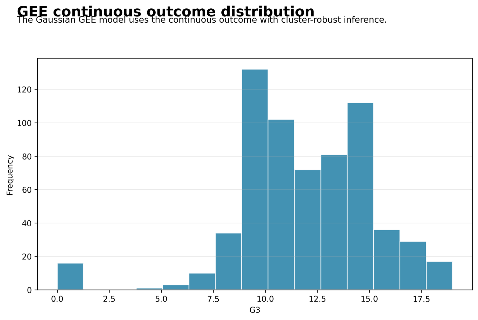
The Python continuous GEE uses G3, the final grade, as the outcome. The original file contained 649 rows, while 645 complete rows entered the model after variables required for clustering and regression were checked. G3 ranges from 0 to 19. Its mean in the full student data is approximately 11.906, with a standard deviation close to 3.231.
The histogram is concentrated between grades 8 and 16. The tallest interval is around 9–10, with roughly 130 observations; intervals around 10–11 and 14–15 also contain more than 100 observations. A small group of approximately 16 students has G3 near zero. These unusually low outcomes matter because several are much lower than predictions based on G1 and G2 and later produce residuals below −8.
This chart documents the scale analyzed by the Gaussian identity-link model. The fitted exchangeable GEE has RMSE = 1.2436, MAE = 0.7817, and pseudo-R² 0.8521. Therefore, even though the outcome includes a small lower-tail group, the marginal mean model reproduces most final grades with an average absolute error below one grade point.
Python Chart 2: Constructed Cluster-Size Distribution
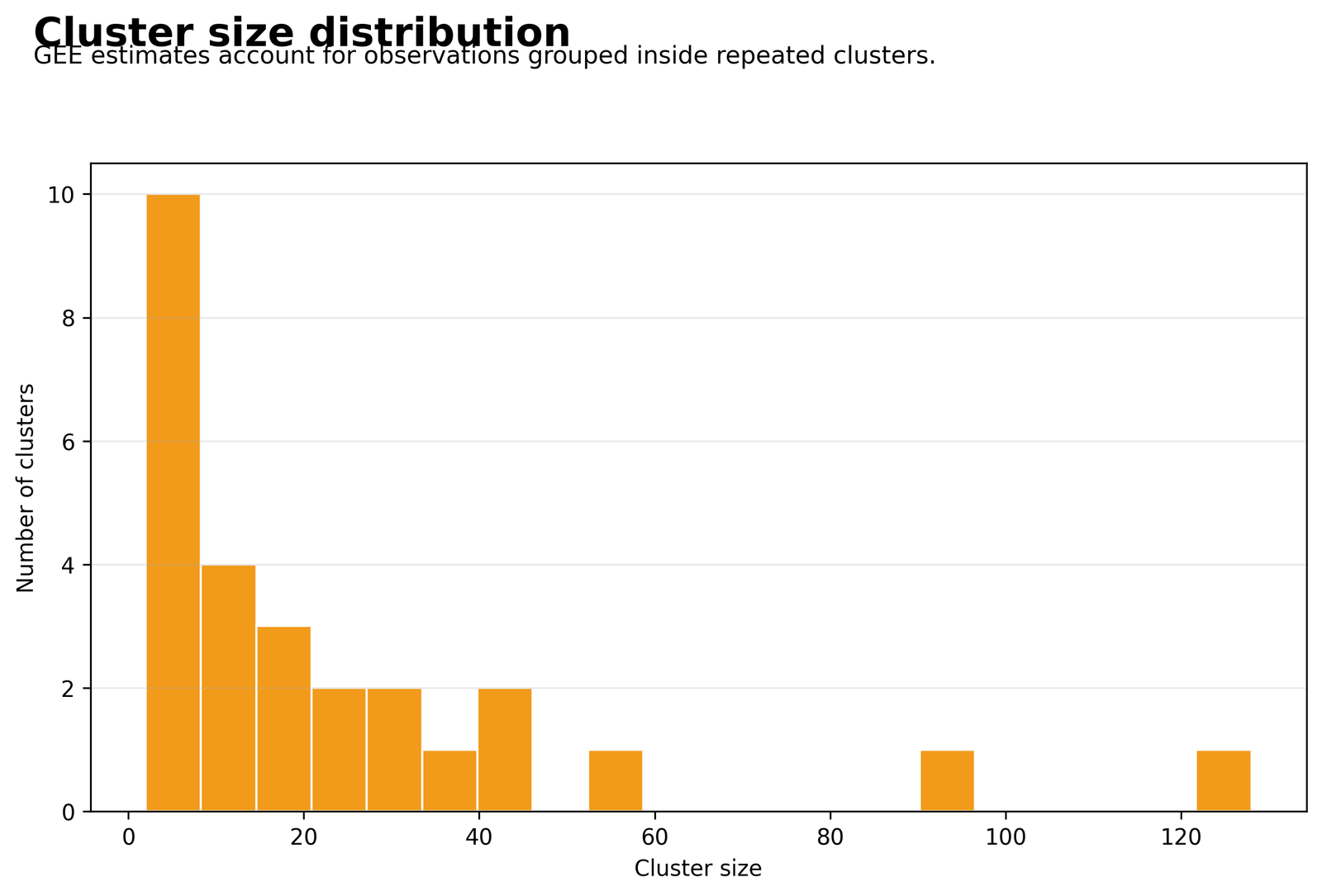
Python creates gee_cluster from the combination of school, sex, address, famsize, and Pstatus. After complete-case filtering, the model includes 27 clusters. Cluster size is highly unequal: the minimum is 2, the maximum is 128, and the mean is 23.8889 observations per cluster.
The histogram shows that most clusters are small. Approximately 10 clusters fall in the smallest size interval, four clusters are in the next interval, and three are in the following interval. Only a few clusters exceed 40 observations. The two largest clusters contain 92 and 128 students, while several clusters contain only two to five students.
This imbalance is important for robust inference. GEE can accommodate unequal cluster sizes, but very large clusters can contribute more information to the estimating equations, while very small clusters provide limited information about within-cluster association. The reported sandwich standard errors account for clustering, yet cluster influence and sensitivity to the largest groups should still be examined.
Python Chart 3: Observed vs Fitted Exchangeable GEE Values
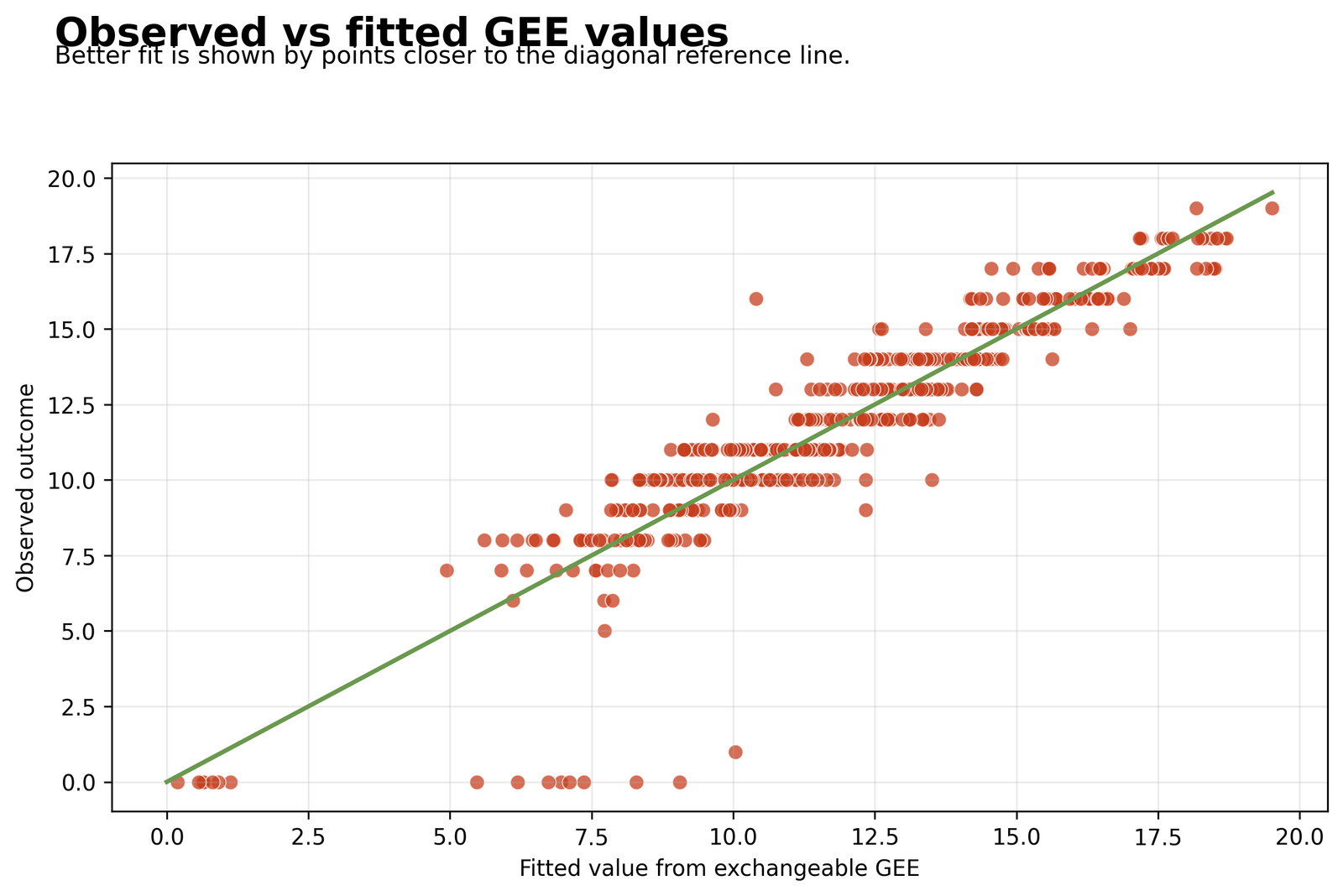
The observed-versus-fitted chart uses fitted marginal means from the exchangeable Gaussian GEE. Most of the 645 observations lie near the diagonal from fitted values of approximately 7 to 19. The step-like horizontal rows occur because observed G3 is integer-valued, whereas fitted values are continuous.
The close diagonal alignment agrees with pseudo-R² 0.8521, RMSE 1.2436, and MAE 0.7817. The model’s two strongest predictors are G2 and G1. For the exchangeable model, G2 has B = 0.8779 and G1 has B = 0.1344. Holding the other variables constant, one additional G2 grade point is associated with approximately 0.878 additional G3 points in the population-average outcome, while one additional G1 point is associated with approximately 0.134 additional G3 points.
The main departures occur among observed G3 = 0 cases that receive fitted values around 5.5 to 10. One observed value near 1 is also fitted near 10. These cases explain the large negative residuals and show why excellent overall fit does not imply that every student is predicted accurately.
Python Chart 4: Residuals vs Fitted Values
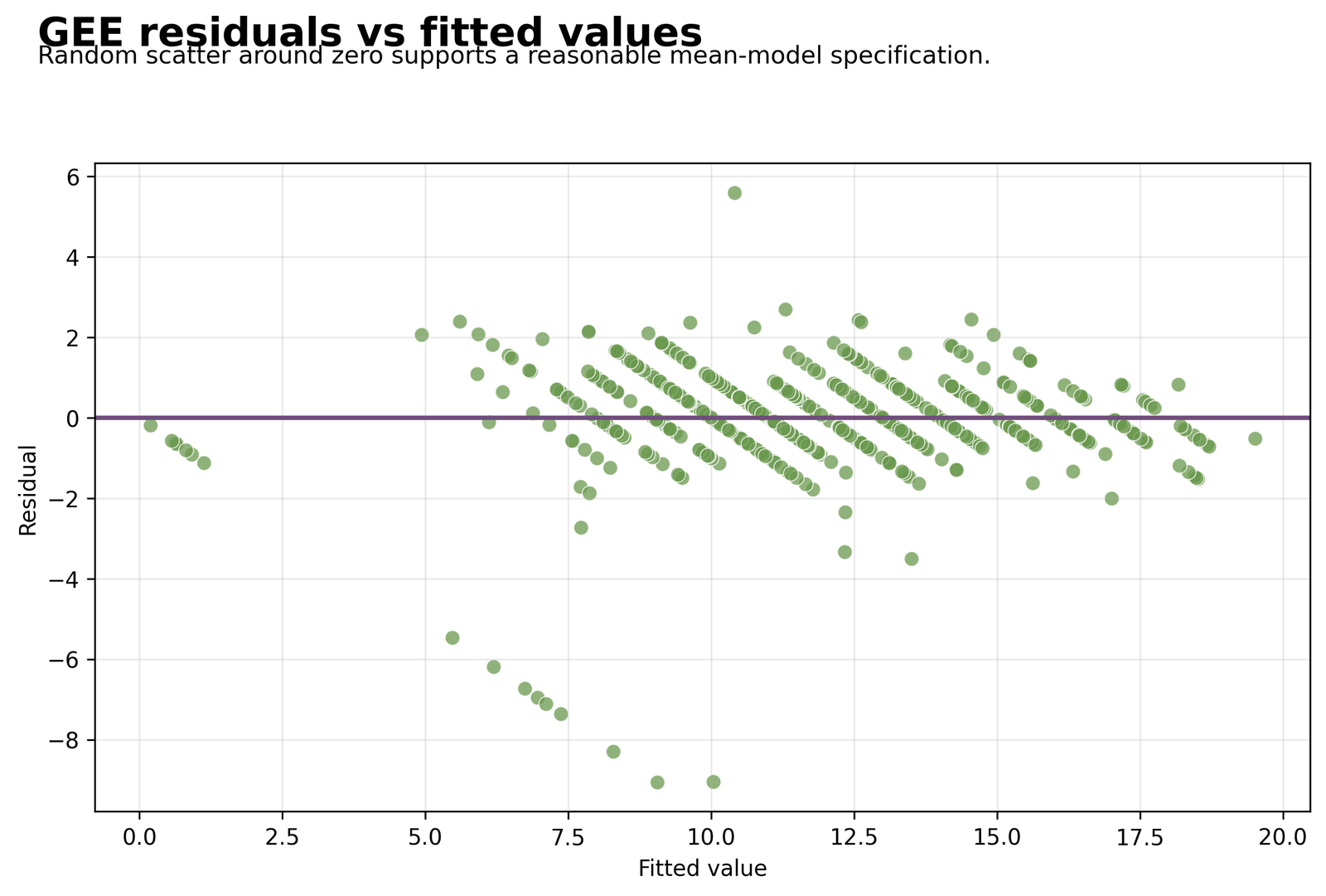
Python residuals are calculated as observed G3 minus the exchangeable GEE fitted marginal mean. Most residuals are distributed between approximately −2 and +2.5 around the horizontal zero line. This central band corresponds with MAE 0.7817 and indicates limited average bias for most observations.
Several large negative residuals occur between fitted values of approximately 5.5 and 10. The most extreme points reach about −9.2, −9.0, and −8.3. These represent students whose final grade was far below the marginal mean predicted from G1, G2, studytime, failures, absences, age, school, sex, and address. A large positive residual near +5.6 at a fitted value close to 10 represents an observed final grade much higher than predicted.
The residuals show diagonal stripes because the observed outcome takes integer values. No strong smooth curve is visible through the central cloud, which supports the linear mean specification. However, the heavy negative tail should be investigated through studentized residuals, Cook’s distance, Mahalanobis distance, and influence diagnostics.
Python Chart 5: Exchangeable GEE Coefficients with Robust 95% CIs
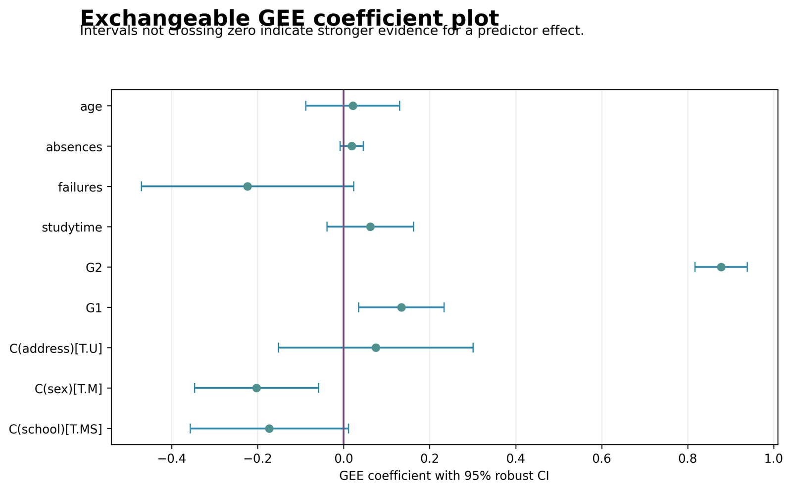
The coefficient plot reports population-average exchangeable GEE coefficients with robust sandwich 95% confidence intervals. The strongest effect is G2: B = 0.8779, robust SE 0.0310, z = 28.2876, p < .001, 95% CI [0.8171, 0.9388]. G1 is also significant: B = 0.1344, robust SE 0.0507, z = 2.6519, p = .0080, 95% CI [0.0351, 0.2337].
The male-versus-female contrast is significant and negative: B = −0.2026, robust SE 0.0735, z = −2.7556, p = .0059, 95% CI [−0.3468, −0.0585]. After the remaining variables are controlled, the population-average G3 for male students is about 0.203 grade points lower than for female students under this coded model.
The MS-versus-GP school contrast is negative but narrowly crosses zero: B = −0.1727, p = .0657, CI [−0.3566, 0.0112]. Address_U has B = 0.0748, p = .5162; studytime B = 0.0623, p = .2252; failures B = −0.2234, p = .0760; absences B = 0.0187, p = .1758; and age B = 0.0212, p = .7031. Their robust intervals cross zero, so they are not significant at α = .05.
Python Chart 6: Independence vs Exchangeable Working Correlation
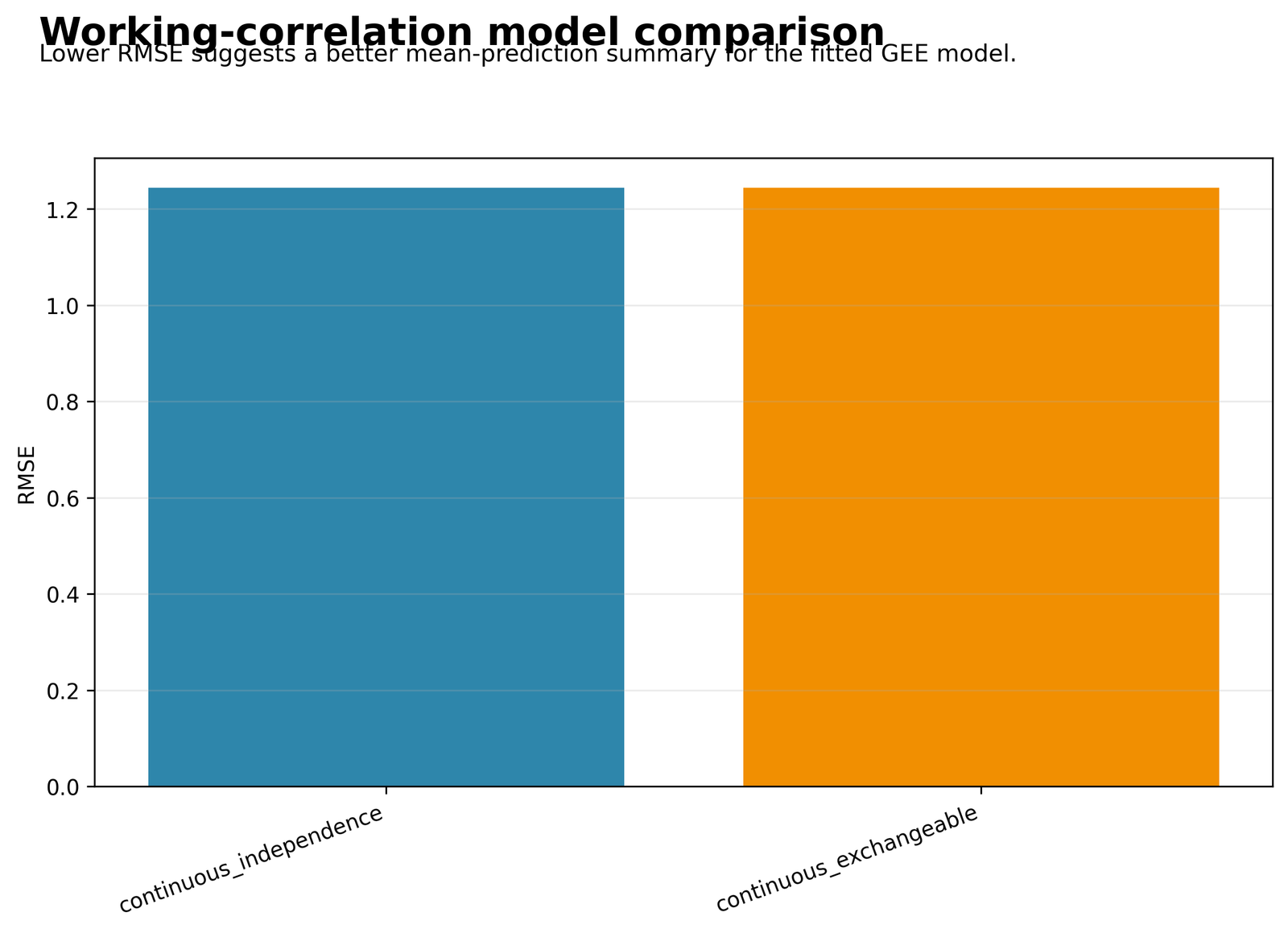
The working-correlation comparison shows almost identical fitted RMSE values. The independence model has RMSE = 1.243561 and the exchangeable model has RMSE = 1.243635. Their difference is only about 0.000073. MAE slightly favors exchangeable: 0.781680 compared with 0.782135 for independence.
The estimated exchangeable working-correlation parameter is −0.00505, which is extremely close to zero. This means that, under the constructed cluster definition, the estimated average residual association among observations within a cluster is negligible after the model predictors are included. It explains why the two fitted-value summaries and coefficient estimates are nearly identical.
A working correlation near zero does not make GEE unnecessary. Robust sandwich inference remains useful when the analyst wants cluster-robust population-average estimates and the independence structure may be misspecified. Nevertheless, this result should be reported honestly: for the Python constructed clusters, exchangeable dependence contributes almost no estimated correlation beyond the marginal mean model.
Python Chart 7: Cluster-Level Mean G3 Outcomes
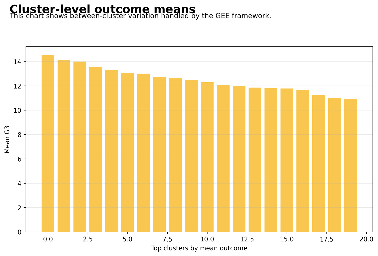
The cluster-mean chart ranks the highest cluster-level G3 means among the 27 constructed clusters. The highest displayed mean is 14.50 for a cluster containing four students. Other high means include 14.1429 for a seven-student cluster, 14.00 for a two-student cluster, 13.5385 for a 13-student cluster, and 13.3047 for the largest 128-student cluster.
At the lower end of the complete cluster table, means include 6.6667 for a three-student cluster, 8.50 for a 28-student cluster, 8.80 for a five-student cluster, and 9.00 for another five-student cluster. The overall mean outcome across the modeled rows is approximately 11.6270. Cluster pass rates range from 0.40 to 1.00, with an average cluster pass rate of approximately 0.8194.
Small clusters can produce extreme means because only a few observations determine the average. Therefore, the highest bar should not be assumed to represent the most consistently successful population. Cluster size, within-cluster standard deviation, and pass rate should be interpreted together. GEE estimates population-average coefficients without introducing a random intercept for each cluster.
Python Chart 8: Binary GEE Calibration by Predicted-Probability Group
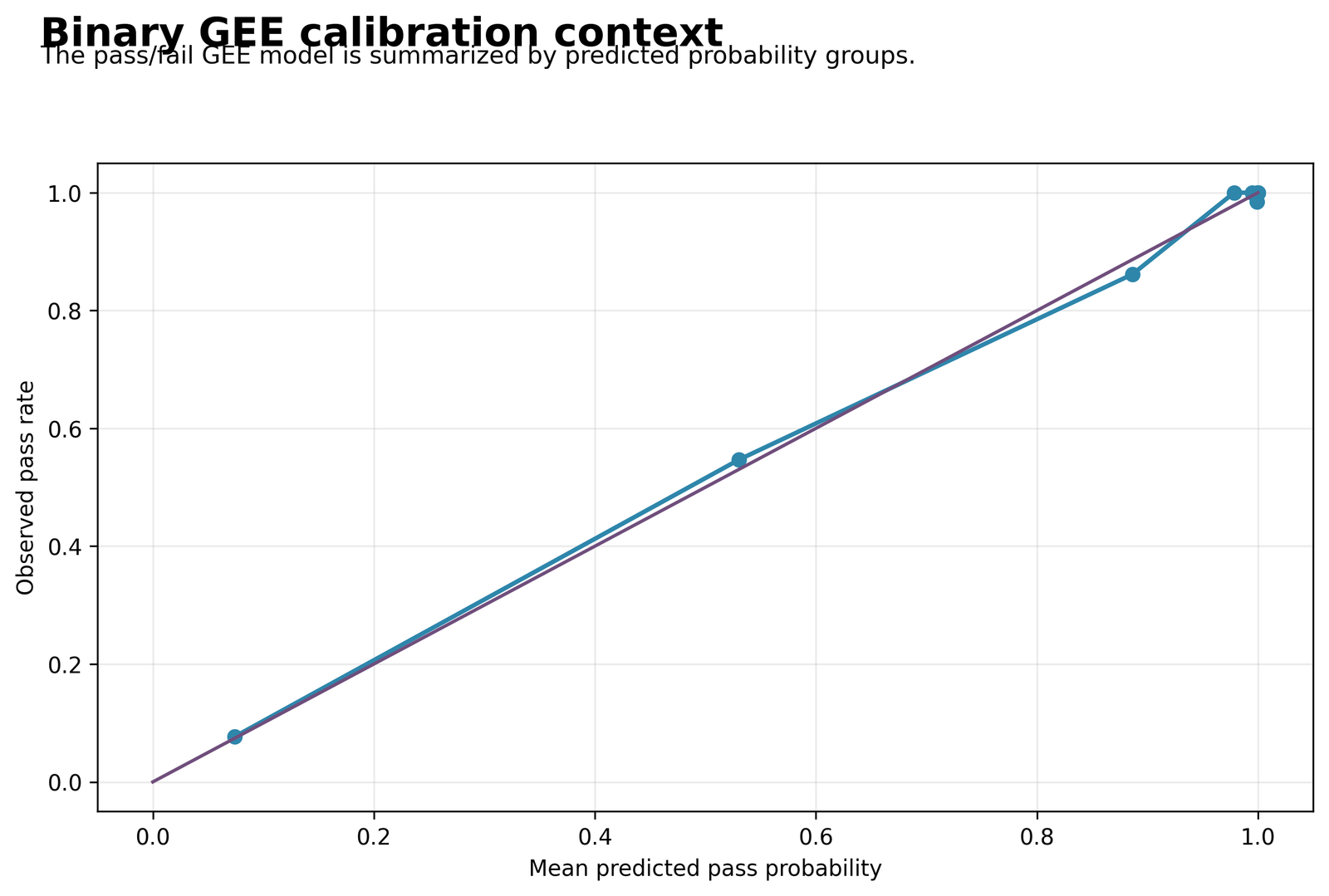
The binary calibration chart summarizes a separate binomial exchangeable GEE in which gee_pass = 1 when G3 ≥ 10 and 0 otherwise. Predicted probabilities are grouped, and each point compares the mean predicted probability with the observed pass rate. Points close to the diagonal indicate good grouped calibration.
The lowest-risk group has a mean predicted probability close to 0.08 and an observed pass rate near 0.07. A middle group is around 0.53 predicted and 0.55 observed. A high-risk group is around 0.89 predicted and 0.86 observed. The highest groups have predicted probabilities from approximately 0.98 to 1.00 and observed rates from approximately 0.98 to 1.00.
The binomial GEE coefficients show that G1 and G2 strongly increase population-average pass odds. G1 has B = 0.6248, p = .000108, giving OR = 1.868. G2 has B = 1.5438, p < .001, giving OR = 4.682. Age is positive, B = 0.4316, p = .00448, OR = 1.540. MS school and male sex have significant negative coefficients. Calibration is visually strong, but the chart should be supplemented with discrimination and classification statistics when the binary model is used for prediction.
Binary Generalized Estimating Equations Interpretation
The Python workbook also contains a binomial exchangeable GEE for gee_pass, coded 1 when G3 is at least 10. The model uses the same predictors and constructed cluster ID. Coefficients are log odds; exponentiated values are population-average odds ratios.
| Term | B | p | Approximate OR | 95% Log-Coefficient CI | Interpretation |
|---|---|---|---|---|---|
| school: MS vs GP | −1.0604 | .00040 | 0.346 | [−1.6470, −0.4738] | Lower population-average pass odds for MS. |
| sex: M vs F | −0.7116 | .04019 | 0.491 | [−1.3915, −0.0318] | Lower adjusted pass odds for male students. |
| address: U vs R | −0.2008 | .53338 | 0.818 | [−0.8327, 0.4311] | Not significant. |
| G1 | 0.6248 | .000108 | 1.868 | [0.3085, 0.9410] | Each point increases marginal pass odds. |
| G2 | 1.5438 | <.001 | 4.682 | [0.9920, 2.0956] | Strongest positive pass predictor. |
| studytime | 0.1285 | .5620 | 1.137 | [−0.3058, 0.5628] | Not significant. |
| failures | −0.3236 | .2651 | 0.724 | [−0.8927, 0.2456] | Not significant after adjustment. |
| absences | −0.0316 | .4321 | 0.969 | [−0.1104, 0.0472] | Not significant. |
| age | 0.4316 | .00448 | 1.540 | [0.1340, 0.7293] | Significant positive adjusted association. |
The model’s calibration plot is close to the diagonal. However, a full binary evaluation should also report ROC AUC, sensitivity, specificity, confusion counts and threshold choice. The supplied populated workbook focuses mainly on continuous GEE, while the second Excel workbook provides a template for binary GEE coefficients and predictions.
R Repeated-Grade GEE Design
R converts each student’s G1, G2 and G3 values into a long dataset. Every student becomes one cluster identified by subject_id and contributes three repeated rows. The resulting analysis contains 1,947 observations across 649 clusters.
The Gaussian identity-link model compares independence and exchangeable structures. Exchangeable assumes the same average correlation among G1, G2 and G3 within a student. The estimated rho is 0.8095698, supporting strong repeated-score dependence.
R GEE Model-Fit and Marginal Coefficient Results
R Fit Summary
| Statistic | Independence | Exchangeable |
|---|---|---|
| Repeated observations | 1,947 | 1,947 |
| Student clusters | 649 | 649 |
| Parameters | 12 | 12 |
| Working rho | 0 | 0.8095698 |
| Scale parameter | 6.445688 | 6.445688 |
| RMSE | 2.531 | 2.531 |
| MAE | 1.901495 | 1.901495 |
| Quasi-information | 3640.0248 | 3640.0248 to displayed precision |
R Exchangeable Marginal Coefficients
| Term | B | Robust SE | Wald χ² | p | 95% CI |
|---|---|---|---|---|---|
| Intercept | 9.9838 | 1.3942 | 51.2780 | <.001 | [7.2512, 12.7164] |
| grade_time linear | 0.3585 | 0.0505 | 50.3864 | <.001 | [0.2595, 0.4574] |
| grade_time quadratic | 0.0673 | 0.0333 | 4.0811 | .04336 | [0.0020, 0.1326] |
| studytime | 0.4640 | 0.1197 | 15.0261 | .000106 | [0.2294, 0.6986] |
| failures | −1.5047 | 0.1612 | 87.0882 | <.001 | [−1.8208, −1.1887] |
| absences | −0.0671 | 0.0217 | 9.5817 | .00197 | [−0.1096, −0.0246] |
| age | 0.0451 | 0.0808 | 0.3113 | .57685 | [−0.1133, 0.2034] |
| Medu | 0.2732 | 0.1179 | 5.3702 | .02048 | [0.0421, 0.5043] |
| Fedu | 0.1576 | 0.1159 | 1.8504 | .17373 | [−0.0695, 0.3848] |
| school: MS vs GP | −1.2579 | 0.2421 | 26.9964 | <.001 | [−1.7324, −0.7834] |
| sex: M vs F | −0.5800 | 0.1980 | 8.5860 | .00339 | [−0.9680, −0.1921] |
| address: U vs R | 0.2806 | 0.2354 | 1.4214 | .23318 | [−0.1807, 0.7419] |
R Chart-by-Chart Interpretation with Real Data Values
The R report contains eight repeated-measures figures. The following discussions use the exact number of observations and clusters, repeated-score means, marginal coefficients, robust confidence intervals, working correlation, error values and visible chart ranges.
R Chart 1: Repeated G1, G2 and G3 Outcome Distribution
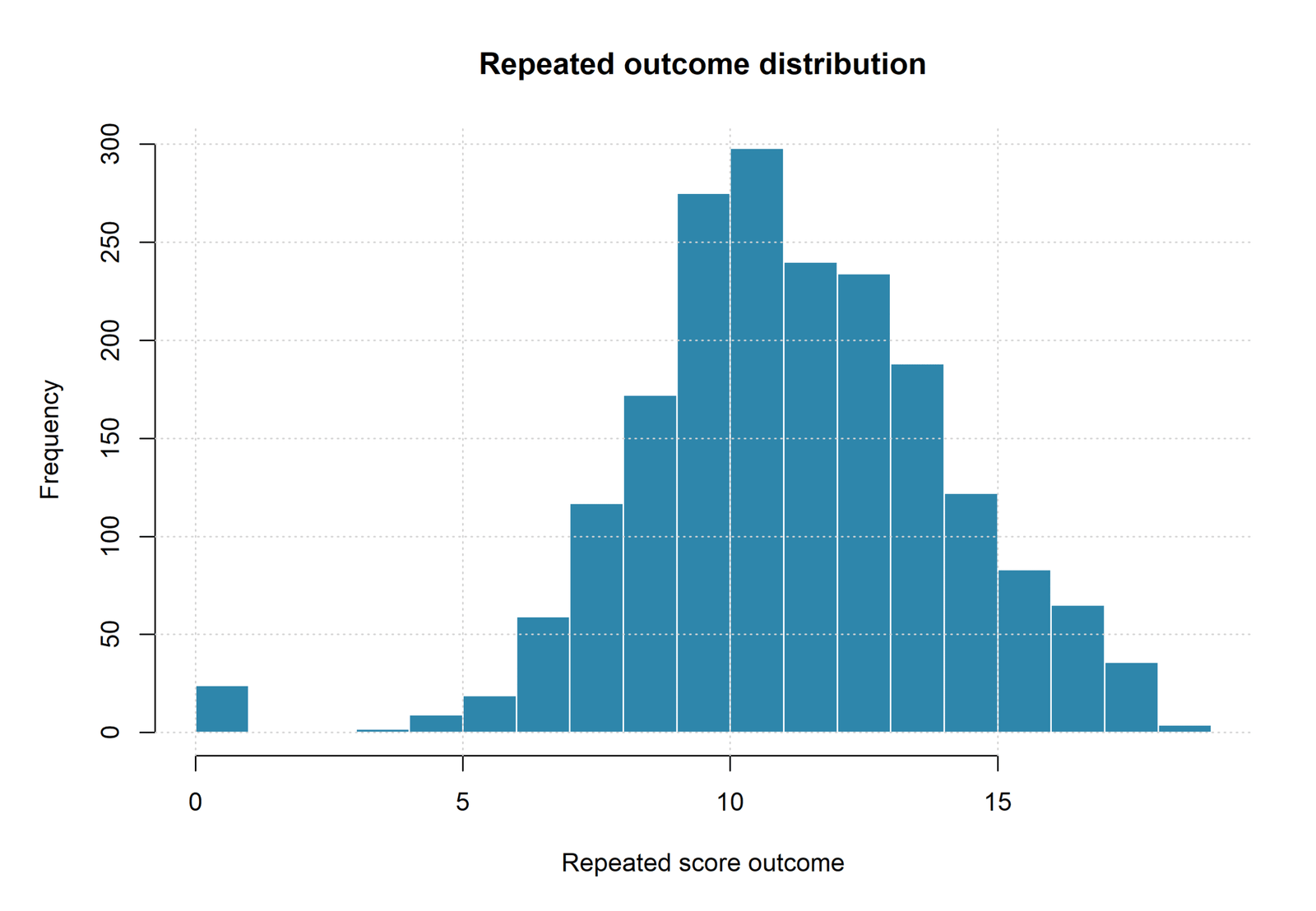
The R workflow restructures each student’s G1, G2, and G3 scores into a long repeated-outcome dataset. The model therefore uses 1,947 repeated observations nested within 649 student clusters, exactly three score occasions per student. The repeated score ranges from 0 to 19 and is concentrated around approximately 9 to 14.
The histogram’s tallest bars contain close to 300 repeated scores around grade 10 and about 275 around grade 9. Frequencies gradually decline above approximately 13, while a small group of roughly 20–25 repeated values occurs at zero. This distribution combines the three grade occasions rather than showing G3 alone.
The R exchangeable GEE estimates a strong within-student correlation of rho = 0.80957. That value is expected because G1, G2, and G3 from the same student are closely related repeated academic measurements. This design is conceptually different from the Python constructed-cluster analysis, where rho is approximately zero.
R Chart 2: Mean Repeated Score Profile Across Grade Time
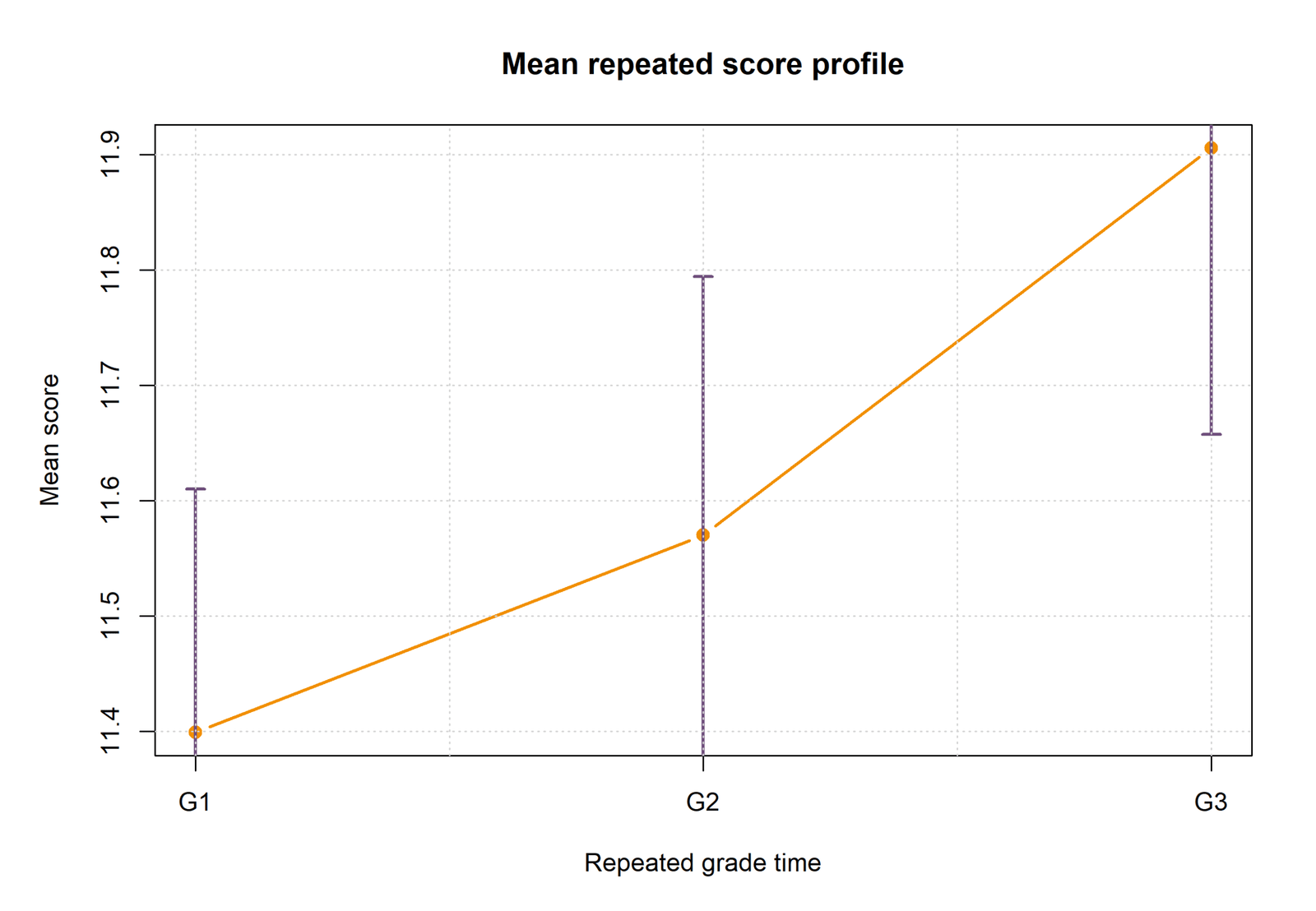
The mean-profile chart displays the average score at each repeated grade occasion. The mean is approximately 11.399 at G1, 11.570 at G2, and 11.906 at G3. The increase from G1 to G2 is about 0.171 points, while the increase from G2 to G3 is about 0.336 points. Across the first and final periods, the average rises by approximately 0.507 points.
The vertical intervals show the spread around each mean. They overlap substantially, demonstrating that the mean changes are small relative to between-student variation. The GEE time effect is represented with orthogonal polynomial contrasts. The linear time component is significant: B = 0.35846, robust SE 0.05050, Wald χ² 50.388, p < .001, CI [0.25948, 0.45743].
The quadratic component is also statistically significant but smaller: B = 0.06731, robust SE 0.03332, Wald χ² 4.081, p = .04336, CI [0.00201, 0.13261]. This indicates that the upward change is not perfectly constant: the increase from G2 to G3 is larger than the increase from G1 to G2.
R Chart 3: Observed vs Fitted Repeated GEE Values
The R observed-versus-fitted chart contains all 1,947 repeated scores. Fitted marginal means range from approximately 5.5 to 14.8, while observed scores range from 0 to 19. The green reference line shows perfect agreement. The model captures the central trend, but the cloud is more dispersed than in the Python G3-only model.
The reported R exchangeable GEE has RMSE = 2.531 and MAE = 1.901495. These errors are larger than the Python G3-only values because the R model predicts all three repeated grades using time and background variables rather than using G1 and G2 as direct predictors of G3. The two models answer different questions and their RMSE values must not be compared as though they were the same specification.
The chart shows many observations close to the fitted trend, especially around scores 9–15. However, several observed zero scores receive fitted means near 9–13, and some high observed scores of 17–19 receive fitted means near 11–14. This dispersion reflects substantial individual variation that a population-average GEE is not designed to model with subject-specific random effects.
R Chart 4: Repeated-Outcome Residuals vs Fitted Values
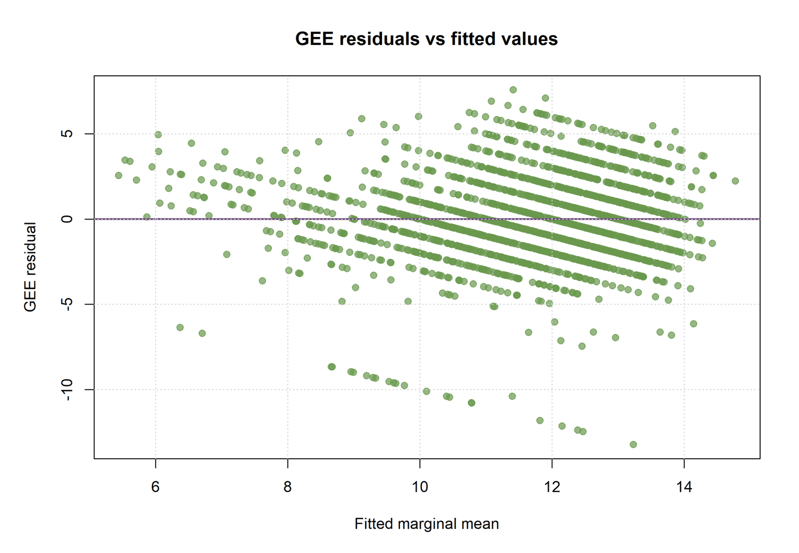
The repeated-outcome residual plot shows residuals from approximately −13 to +7.5. Most observations fall between −5 and +5, with dense diagonal stripes created by integer observed scores. The zero line passes through the middle of the main cloud, but the negative tail is longer than the positive tail.
Large negative residuals occur when observed repeated scores are zero or very low while fitted marginal means are around 9–13. The most extreme residual is approximately −13. Positive residuals reach about +7.5 when an observed grade is substantially higher than its population-average prediction.
The residual scale is consistent with RMSE = 2.531 and MAE = 1.901495. These values are not evidence that GEE failed; they show that a marginal model based on time and background characteristics leaves considerable individual-level heterogeneity. Subject-specific prediction would require a mixed-effects model rather than GEE alone.
R Chart 5: Exchangeable GEE Residual Distribution
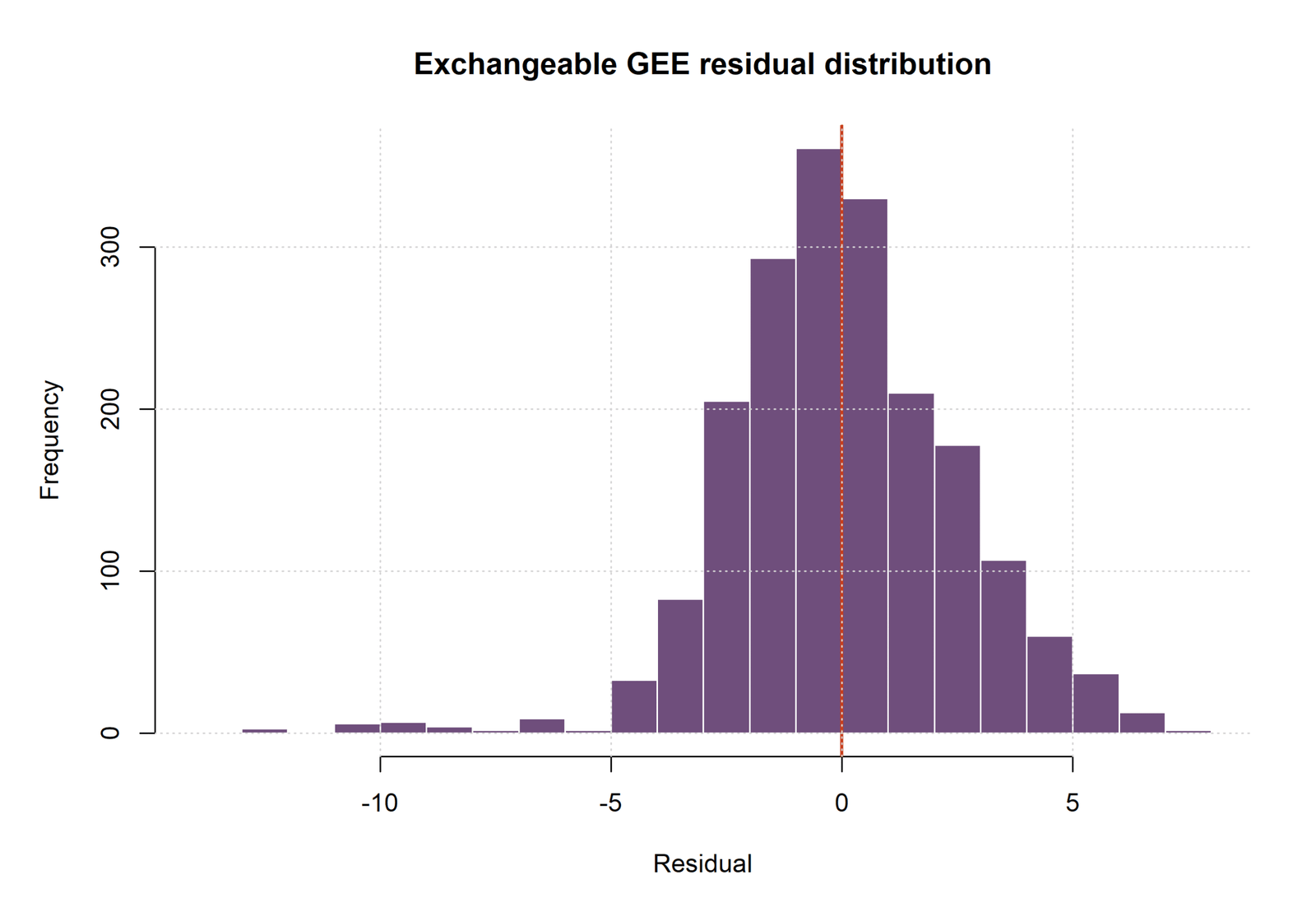
The R residual histogram is centered near zero, with the tallest interval containing approximately 350 residuals immediately below zero and another interval containing more than 320 immediately above zero. More than 200 observations occur in each of several neighboring bins from approximately −3 to +3.
The left tail extends below −10 and reaches approximately −13, while the right tail extends to about +8. The distribution is therefore negatively skewed by rare very low observed grades. The vertical zero line passes through the central concentration, supporting approximate centering of the marginal mean errors even though the tails are not symmetric.
For descriptive diagnostics, the distribution can be supplemented with a Q–Q plot, P–P plot, skewness and kurtosis check, and outlier review. Robust sandwich inference reduces reliance on perfectly specified variance, but the mean model and influential observations still require examination.
R Chart 6: Working-Correlation Quasi-Information Comparison
The R working-correlation comparison reports a quasi-information value of 3640.0248 for both independence and exchangeable structures to the displayed precision. The bars are therefore visually equal. The report states that exchangeable has the lower value, but the difference is smaller than the rounded display can show.
The estimated exchangeable correlation is rho = 0.8095698, indicating strong average correlation among G1, G2, and G3 from the same student. Independence sets rho to zero. Even when the quasi-information values are almost indistinguishable, exchangeable is substantively plausible because repeated grades from the same student are strongly associated.
Working-correlation choice affects efficiency rather than the basic meaning of the marginal coefficients. Robust sandwich standard errors protect inference against some correlation misspecification when the number of independent clusters is adequate. With 649 students, the R analysis has far more clusters than the Python constructed-cluster model and provides a strong basis for robust marginal inference.
R Chart 7: Marginal Coefficients with Robust 95% CIs
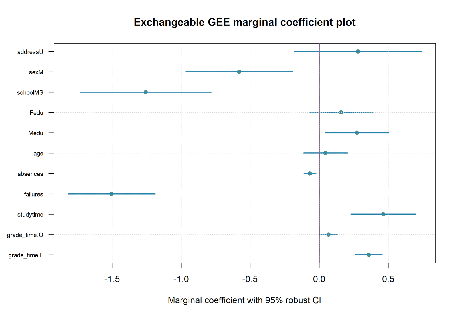
The R coefficient plot presents exchangeable GEE population-average effects with robust confidence intervals. The linear grade-time contrast is positive and significant: B = 0.35846, CI [0.25948, 0.45743]. The quadratic contrast is smaller but significant: B = 0.06731, CI [0.00201, 0.13261].
Studytime is positive: B = 0.46400, robust SE 0.11970, p = .000106, CI [0.22939, 0.69861]. Failures has the strongest negative effect: B = −1.50474, p < .001, CI [−1.82077, −1.18871]. Absences is also significantly negative: B = −0.06713, p = .00197, CI [−0.10964, −0.02462].
Mother’s education is positive and significant: B = 0.27320, p = .02048, CI [0.04213, 0.50426]. Father’s education is not significant: B = 0.15763, p = .17373. MS school is negative, B = −1.25793, p < .001; male sex is negative, B = −0.58003, p = .00339. Address_U and age are not significant because their robust intervals cross zero.
R Chart 8: Student-Cluster Observed vs Fitted Means
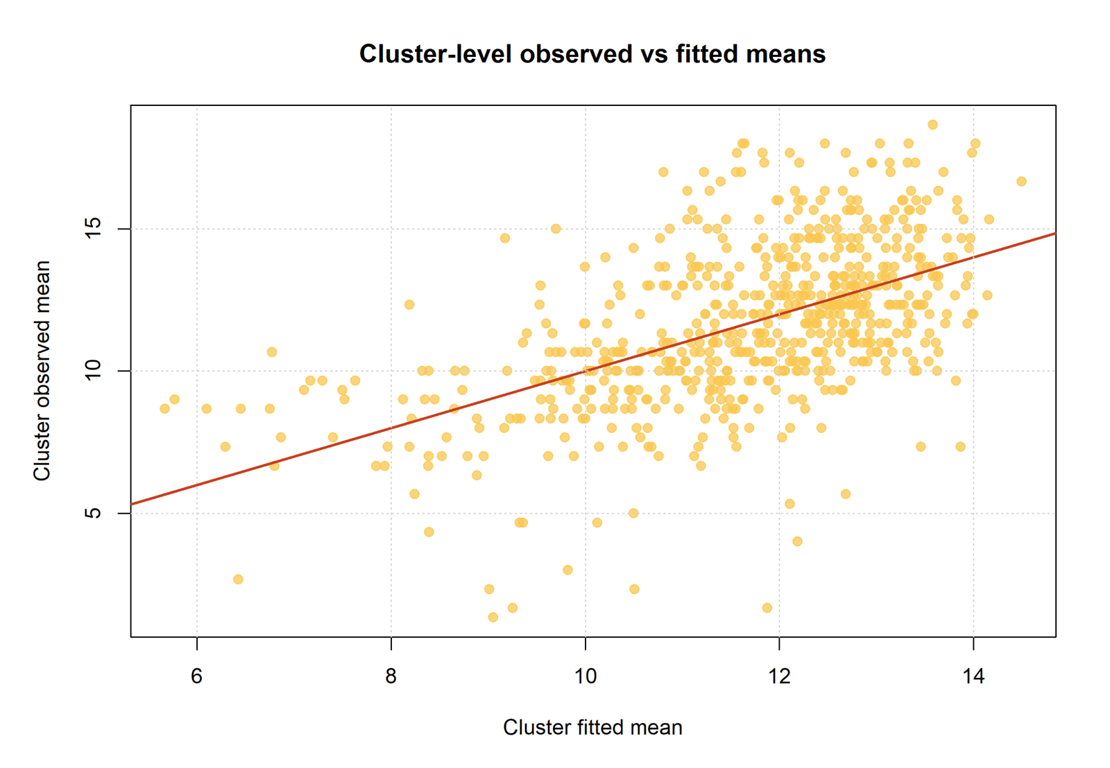
Each point in this chart represents one of the 649 student clusters. The horizontal axis is the student’s fitted mean across the three repeated score occasions, and the vertical axis is the observed mean of G1, G2, and G3. Fitted cluster means range from approximately 5.5 to 14.5, while observed means range from roughly 1.3 to 18.5.
The upward trend shows that students with higher fitted marginal means generally have higher observed average grades. The red line rises from approximately an observed mean of 5.5 at a fitted mean of 5.5 to about 14.8 at a fitted mean of 14.8. However, considerable vertical dispersion remains, especially among fitted means from 10 to 14.
This is expected for a population-average GEE. It estimates marginal effects and robust uncertainty but does not add a student-specific random intercept. Two students with similar background variables can therefore have different observed grade profiles. The chart supports useful average prediction while demonstrating why GEE coefficients should not be described as individualized forecasts.
How to Choose a GEE Working Correlation
The working correlation should reflect how measurements are expected to relate within clusters. Independence is a useful robust baseline. Exchangeable is appropriate when all within-cluster pairs can reasonably share one average correlation. AR(1) is more suitable when measurements are ordered and correlations should decline with time separation.
For the R data, only three grade occasions are available. Exchangeable rho = 0.8096 summarizes their strong common correlation. An AR(1) structure could distinguish adjacent and more separated grades, but with only three occasions the evidence may be limited.
For Python’s constructed clusters, rho = −0.0051. The mean predictions are nearly identical under independence and exchangeable. Independence may therefore be sufficient for efficiency, but the robust covariance should still be retained if clustering is part of the design.
Working-correlation choice should be based on scientific structure, fit summaries, coefficient stability and robust standard errors—not only the smallest displayed RMSE.
Cluster Definition and Cluster-Size Issues
A valid cluster ID groups observations that may be correlated and separates observations that can reasonably be treated as independent. A subject ID is natural for repeated measurements. A school ID is natural when students are nested in schools. A combined key created from several demographic categories may be useful for demonstration but should not replace a true design-based cluster when one exists.
Number of Clusters
R has 649 clusters and is well suited to large-sample sandwich inference. Python has 27 clusters, which is relatively small. Small-cluster corrections or alternative approaches may be considered when inference is sensitive.
Unequal Cluster Sizes
Python cluster sizes range from 2 to 128. The largest cluster contains nearly 20% of the 645 modeled observations. Analysts should conduct sensitivity checks that remove or down-weight unusually influential clusters and compare coefficient stability.
Singleton and Very Small Clusters
The Python minimum is two, so there are no singleton clusters in the reported model. Several two-, three-, four- and five-observation clusters remain. They contribute to the marginal mean but provide limited information for estimating within-cluster correlation.
GEE Residuals, Influence and Diagnostic Checks
GEE is robust to some covariance misspecification, but the mean model still requires diagnostic evaluation. Important checks include residual-versus-fitted patterns, extreme observations, influential clusters, link and family suitability, missingness, multicollinearity and coefficient stability across working structures.
Residual Pattern
Python residuals are mostly within ±2 but include several values near −9. R repeated-outcome residuals span approximately −13 to +7.5. The larger R errors reflect a different outcome structure and predictor set, not simply worse software.
Influential Clusters
Python clusters of 128 and 92 observations deserve special attention. Refit the model excluding each large cluster and compare G1, G2 and sex coefficients, robust SEs and working rho.
Multicollinearity
G1 and G2 are strongly related. Review multicollinearity, variance inflation factors and tolerance. GEE robust standard errors do not solve unstable coefficient separation caused by highly overlapping predictors.
Mean-Model Nonlinearity
Residual curvature may indicate transformations or smooth terms. Useful internal guides include log transformation, square-root transformation and Box–Cox transformation.
Validation
GEE coefficients target marginal association rather than machine-learning prediction. When prediction matters, use cluster-level cross-validation so all observations from one cluster remain in the same fold. Randomly splitting repeated rows across training and test sets would leak subject information.
Worked Excel Files for Generalized Estimating Equations
Two Excel workbooks were supplied. They serve different purposes and should not be treated as duplicate files.
Populated Continuous GEE Workbook
The populated workbook includes Summary, Model_Coefficients, Worked_Data, Cluster_Summary and Instructions sheets. It documents 649 dataset rows, 645 model rows, 27 clusters, G3 as the outcome, and exchangeable Gaussian GEE as the main model.
| Workbook Result | Value |
|---|---|
| Exchangeable rho | −0.0050503 |
| Exchangeable pseudo R² | 0.8521047 |
| Exchangeable RMSE | 1.2436346 |
| Exchangeable MAE | 0.7816798 |
| Clusters / mean size | 27 / 23.8889 |
| Minimum / maximum size | 2 / 128 |
| Mean modeled outcome | 11.6270 |
| Mean cluster pass rate | 0.81935 |
The Worked_Data sheet contains row-level fitted values, residuals and cluster identifiers. The Model_Coefficients sheet stores both independence and exchangeable continuous coefficients and binomial exchangeable coefficients. The Cluster_Summary sheet contains size, mean G3, standard deviation and pass rate for every cluster.
Binary GEE Template Workbook
The second workbook contains README, Setup, Data_Input, Coefficient_Input, Prediction_Template, Diagnostics and Report_Template sheets. It is an editable companion for a binomial logit-link GEE. The default outcome is gee_pass, the cutoff is 10, the main working correlation is exchangeable and the default cluster rule uses school, address, family size and parental status.
The Coefficient_Input sheet accepts B, robust SE, Wald z, p-value, log-confidence limits and odds ratios. The Prediction_Template calculates a population-average predicted probability for a new covariate pattern. This prediction does not include an individual random effect because GEE is marginal rather than subject-specific.
Core Excel Formulas
Binary outcome:
=IF(G3_cell>=Setup!$B$6,1,0)

Cluster key:
=school&"|"&sex&"|"&address&"|"&famsize&"|"&Pstatus

Continuous fitted value:
=Intercept
 + B_schoolMS*school_MS
 + B_sexM*sex_M
 + B_addressU*address_U
 + B_G1*G1
 + B_G2*G2
 + B_studytime*studytime
 + B_failures*failures
 + B_absences*absences
 + B_age*age

Residual:
=Observed_G3-Fitted_G3

Binary linear predictor:
=SUMPRODUCT(Predictor_Values,Coefficient_Values)

Predicted probability:
=1/(1+EXP(-Linear_Predictor))

Odds ratio:
=EXP(Coefficient_B)

Robust 95% log-CI:
Lower = B-1.96*Robust_SE
Upper = B+1.96*Robust_SE

Robust 95% OR-CI:
Lower_OR = EXP(Lower_Log_CI)
Upper_OR = EXP(Upper_Log_CI)
Excel limitation: Excel can organize coefficients, predictions, residuals and cluster summaries, but the robust sandwich covariance and iterative GEE estimation should be produced by Python, R or SPSS integration rather than recreated with simple worksheet formulas.
SPSS Generalized Estimating Equations Workflow
SPSS supports GEE through the Generalized Linear Models interface. The analyst specifies the subject variable, optional within-subject variable, outcome distribution, link, predictors, model effects and working-correlation structure.
Continuous Repeated-Score SPSS Setup
Reshape G1, G2 and G3 into long form with variables subject_id, grade_time and gee_score. Use subject_id as the subject variable, grade_time as within-subject, Gaussian distribution, identity link and exchangeable working correlation. Add studytime, failures, absences, age, Medu, Fedu, school, sex and address.
Binary GEE SPSS Setup
Create gee_pass from G3 ≥ 10. Use binomial distribution and logit link. Specify a scientifically meaningful subject or cluster ID, exchangeable or independence working correlation, robust covariance and confidence intervals for exponentiated coefficients.
No GEE-specific SPSS PDF URL was supplied in the current media list, so the article does not invent or link an SPSS output file.
Python, R and SPSS Code for Generalized Estimating Equations
Python Continuous GEE
import pandas as pd
import statsmodels.api as sm
import statsmodels.formula.api as smf
from statsmodels.genmod.cov_struct import Independence, Exchangeable

df = pd.read_csv("dataset.csv")
df["gee_cluster_key"] = (
    df["school"].astype(str) + "|" +
    df["sex"].astype(str) + "|" +
    df["address"].astype(str) + "|" +
    df["famsize"].astype(str) + "|" +
    df["Pstatus"].astype(str)
)
df["gee_cluster"] = pd.factorize(df["gee_cluster_key"])[0] + 1

formula = (
    "G3 ~ G1 + G2 + studytime + failures + absences + age "
    "+ C(school) + C(sex) + C(address)"
)

independence = smf.gee(
    formula=formula,
    groups="gee_cluster",
    data=df,
    family=sm.families.Gaussian(),
    cov_struct=Independence()
).fit()

exchangeable = smf.gee(
    formula=formula,
    groups="gee_cluster",
    data=df,
    family=sm.families.Gaussian(),
    cov_struct=Exchangeable()
).fit()

print(exchangeable.summary())
Python Binary GEE
df["gee_pass"] = (pd.to_numeric(df["G3"]) >= 10).astype(int)

binary_formula = (
    "gee_pass ~ G1 + G2 + studytime + failures + absences + age "
    "+ C(school) + C(sex) + C(address)"
)

binary_gee = smf.gee(
    formula=binary_formula,
    groups="gee_cluster",
    data=df,
    family=sm.families.Binomial(),
    cov_struct=Exchangeable()
).fit()

df["predicted_pass_probability"] = binary_gee.predict(df)
print(binary_gee.summary())
R Repeated-Grade GEE
library(geepack)

df <- read.csv("dataset.csv")
df$subject_id <- seq_len(nrow(df))

long <- reshape(
  df,
  varying = c("G1", "G2", "G3"),
  v.names = "gee_score",
  timevar = "grade_time",
  times = c("G1", "G2", "G3"),
  direction = "long"
)

long$grade_time <- ordered(
  long$grade_time,
  levels = c("G1", "G2", "G3")
)

formula <- gee_score ~ grade_time + studytime + failures +
  absences + age + Medu + Fedu + school + sex + address

gee_ind <- geeglm(
  formula,
  id = subject_id,
  data = long,
  family = gaussian(link = "identity"),
  corstr = "independence"
)

gee_exch <- geeglm(
  formula,
  id = subject_id,
  data = long,
  family = gaussian(link = "identity"),
  corstr = "exchangeable"
)

summary(gee_exch)
SPSS GEE Syntax Pattern
* Long-format repeated grade example.
GENLIN gee_score BY grade_time school sex address
  WITH studytime failures absences age Medu Fedu
  /MODEL grade_time studytime failures absences age Medu Fedu
         school sex address
    DISTRIBUTION=NORMAL LINK=IDENTITY
  /REPEATED SUBJECT=subject_id WITHINSUBJECT=grade_time
    SORT=YES CORRTYPE=EXCHANGEABLE ADJUSTCORR=YES COVB=ROBUST
  /PRINT CPS DESCRIPTIVES MODELINFO FIT SUMMARY SOLUTION
    WORKINGCORR.

OUTPUT SAVE
  OUTFILE='D:\DATA ANALYSIS\H Regression Tests and Models\Generalized Estimating Equations\SPSS_Output\spv\Generalized-Estimating-Equations.spv'.

OUTPUT EXPORT
  /CONTENTS EXPORT=ALL LAYERS=PRINTSETTING MODELVIEWS=PRINTSETTING
  /PDF DOCUMENTFILE='D:\DATA ANALYSIS\H Regression Tests and Models\Generalized Estimating Equations\SPSS_Output\pdf\Generalized-Estimating-Equations-SPSS-Output.pdf'.
APA-Style Reporting for Generalized Estimating Equations
Python Continuous GEE Report
A Gaussian generalized estimating equations model with an identity link was fitted to estimate population-average final-grade effects while accounting for students grouped into 27 constructed clusters based on school, sex, address, family size and parental status. The analysis included 645 complete observations. An exchangeable working correlation was specified and robust sandwich standard errors were used. The estimated working correlation was −.005. The model produced pseudo-R² = .852, RMSE = 1.244 and MAE = 0.782. G2 was positively associated with G3, B = 0.878, robust SE = 0.031, z = 28.29, p < .001, 95% CI [0.817, 0.939]. G1 was also positive, B = 0.134, p = .008, while male sex was negatively associated with G3, B = −0.203, p = .006. The remaining predictors were not statistically significant at α = .05.
R Repeated-Grade GEE Report
A Gaussian identity-link GEE was fitted to 1,947 repeated G1, G2 and G3 observations nested within 649 students. An exchangeable working correlation was used with robust sandwich standard errors. The estimated within-student correlation was ρ = .810. The linear grade-time contrast was positive, B = 0.358, robust SE = 0.050, p < .001, and the quadratic contrast was also significant, B = 0.067, p = .043. Studytime and maternal education were positively associated with repeated grade score, whereas failures, absences, MS school and male sex were negatively associated. The model had RMSE = 2.531 and MAE = 1.901.
Binary GEE Report
A binomial logit-link exchangeable GEE was fitted to predict gee_pass, coded 1 when G3 was at least 10. Robust population-average results indicated that G1, G2 and age increased pass odds, whereas MS school and male sex decreased pass odds. G2 was the strongest predictor, B = 1.544, OR = 4.682, p < .001. Grouped predicted probabilities closely followed observed pass rates across the calibration curve.
Common Generalized Estimating Equations Mistakes
| Mistake | Why It Is Incorrect | Better Practice |
|---|---|---|
| Not naming the cluster variable | The dependence structure cannot be understood. | State gee_cluster or subject_id and explain how it was defined. |
| Treating repeated rows as independent | Standard errors may be misleading. | Use subject ID and a plausible working correlation. |
| Calling GEE coefficients subject-specific | GEE coefficients are marginal population-average effects. | Use population-average wording. |
| Choosing correlation only by RMSE | Working correlation concerns dependence and efficiency. | Use scientific structure, quasi-information and coefficient stability. |
| Assuming robust means assumption-free | Mean misspecification and influential clusters still matter. | Check residuals, predictors, link and influence. |
| Ignoring number of clusters | Sandwich inference may be biased with few clusters. | Report cluster count and consider small-sample corrections. |
| Comparing Python and R RMSE directly | The models use different outcomes and data structures. | Explain each design separately. |
| Using individual-row cross-validation | Repeated observations can leak across folds. | Split by cluster or subject. |
| Interpreting a non-significant working rho as no clustering concern | Robust inference may still be required by design. | Distinguish design clustering from estimated residual correlation. |
| Using an arbitrary cluster key without justification | Clusters should represent a real dependence mechanism. | Prefer subject, school, classroom, household or clinic IDs. |
| Reporting only p-values | Magnitude and uncertainty are hidden. | Report B, robust SE, CI, p and practical interpretation. |
| Adding random-effects wording | GEE does not estimate random intercepts in the standard model. | Use a mixed model when variance components are required. |
Generalized Estimating Equations Downloads
FAQs About Generalized Estimating Equations
What are Generalized Estimating Equations?
GEE is a regression framework for correlated observations that estimates population-average effects using a marginal mean model, working correlation and commonly robust sandwich standard errors.
When should GEE be used?
Use GEE when observations are repeated within subjects or clustered in groups and the research question concerns average population effects.
What is the cluster variable in Python?
Python constructs gee_cluster from school, sex, address, famsize and Pstatus, producing 27 clusters from 645 complete rows.
What is the cluster variable in R?
R uses subject_id. Each of the 649 students contributes G1, G2 and G3, producing 1,947 repeated observations.
Why are the Python and R working correlations so different?
Python uses constructed demographic clusters and estimates rho near zero. R clusters three repeated grades within the same student and estimates a strong rho of 0.8096.
What does exchangeable correlation mean?
It assumes every pair of observations within a cluster shares the same average working correlation.
What does a GEE coefficient mean?
It is a population-average adjusted association. In a Gaussian identity model, it is measured in outcome units; in a logit model, exp(B) is a marginal odds ratio.
Which Python continuous predictors are significant?
G2, G1 and the male-versus-female contrast are significant in the exchangeable Gaussian GEE.
Which R repeated-model predictors are significant?
Linear and quadratic grade time, studytime, failures, absences, Medu, MS school and male sex are significant.
What is the strongest Python predictor?
G2 is strongest, B = 0.8779, robust SE = 0.0310, p < .001.
What is the strongest negative R predictor?
Failures is strongest, B = −1.5047, p < .001.
Is GEE the same as a mixed-effects model?
No. GEE estimates marginal population-average effects. Mixed models estimate subject-specific effects and random-effect variance components.
Does robust covariance fix every model problem?
No. It helps with covariance misspecification but does not correct an incorrect mean model, poor cluster definition, influential clusters or too few clusters.
How many clusters are needed?
More independent clusters generally improve sandwich inference. R has 649 clusters; Python has 27 and therefore requires greater caution.
Can GEE handle a binary outcome?
Yes. The supplementary Python model uses binomial family and logit link for gee_pass.
Can GEE be run in SPSS?
Yes. SPSS GENLIN supports repeated subject structures, outcome families, links, working correlations and robust covariance.
Can Excel estimate GEE directly?
Excel is suitable for organizing coefficients, predictions and summaries, but Python, R or SPSS should perform the iterative GEE and robust covariance estimation.
How should GEE be validated?
Use cluster-level resampling or cross-validation so all observations from the same subject or cluster remain together.

