
Post hoc tests, adjusted p-values and worked example
Pairwise Comparisons After ANOVA: Tests & Examples
Pairwise comparisons after ANOVA identify which group means differ after a significant overall test. Compare Tukey, Bonferroni and Holm adjustments with formulas, a verified example, and SPSS, R, Python and Excel steps.
Quick Answer: Pairwise Comparisons After ANOVA Result
The worked example compares G3 final grade across four studytime groups. The sample contains 649 students. The one-way ANOVA is statistically significant, with the between-groups variation larger than expected from within-group error alone. That means at least one studytime group has a different mean G3 score, so pairwise comparisons are needed.
The group means show the practical pattern. Studytime group 1 has the lowest mean G3 score, about 10.84. Group 2 has a higher mean, about 12.09. Group 4 has a mean near 13.06, and group 3 has the highest mean, about 13.23. The strongest pairwise differences involve group 1 compared with the higher studytime groups.
Final interpretation: Pairwise comparisons after ANOVA show that the lowest studytime group is clearly separated from several higher studytime groups. The highest two groups, especially groups 3 and 4, are close in mean value and should not be described as strongly different unless the adjusted pairwise p-value supports that decision. The correct report should include group means, mean differences, adjusted p-values and the adjustment method used.
Important reporting point: Do not stop at “ANOVA was significant.” A significant ANOVA only says that not all group means are equal. Pairwise comparisons explain exactly where the differences are.
Table of Contents
- What Are Pairwise Comparisons After ANOVA?
- When to Use Pairwise Comparisons After ANOVA
- Pairwise Comparison Formula
- Null and Alternative Hypotheses
- Dataset and Variables Used
- ANOVA Result and Pairwise Decision Table
- Python Chart-by-Chart Interpretation
- R Chart-by-Chart Validation
- SPSS, R, Python and Excel Workflows
- Code Blocks for Pairwise Comparisons After ANOVA
- APA Reporting Wording
- Common Mistakes
- Downloads and Resources
- Related Guides
- FAQs
What Are Pairwise Comparisons After ANOVA?
Pairwise Comparisons After ANOVA are follow-up tests that compare every pair of group means after the overall ANOVA test. If there are four groups, there are six pairwise comparisons. If there are five groups, there are ten pairwise comparisons. The number of comparisons increases quickly as more groups are added.
The purpose is simple. ANOVA tells whether the group means are not all equal, but it does not tell which specific means differ. Pairwise comparisons answer questions like “Is group 1 different from group 2?” and “Is group 3 different from group 4?” Each pair has a mean difference, standard error, confidence interval and p-value.
Because many pairwise tests are performed at the same time, researchers usually adjust p-values. Common adjustment methods include Tukey HSD, Bonferroni, Holm-Bonferroni, Games-Howell, Gabriel, Hochberg’s GT2, Fisher’s LSD and Student-Newman-Keuls. The best method depends on sample size balance, variance assumptions and how strict the researcher wants to be about false positives.
Simple definition: Pairwise comparisons after ANOVA are post hoc tests that compare group means two at a time to find out exactly which groups differ after the overall ANOVA is significant.
Before using pairwise comparisons, review one-way ANOVA, ANOVA assumptions, Levene test, p-values, confidence intervals and effect size.
When to Use Pairwise Comparisons After ANOVA
Use Pairwise Comparisons After ANOVA when the ANOVA includes three or more groups and the overall F test is significant. In this example, the factor is studytime, the dependent variable is G3 final grade, and the four studytime groups create six pairwise comparisons.
| Use Pairwise Comparisons When | Why It Matters | Example in This Guide |
|---|---|---|
| The ANOVA is significant | The overall F test shows that at least one group differs. | G3 differs across studytime groups. |
| There are three or more groups | ANOVA does not show which exact groups differ. | Four studytime groups require six pairwise tests. |
| You need adjusted p-values | Multiple comparisons increase false-positive risk. | Tukey, Bonferroni and Holm-style adjustments can be compared. |
| You need reportable mean differences | Direction and size are as important as significance. | Group 1 is lower than several higher studytime groups. |
When not to use them mechanically: If the ANOVA is not significant and there were no planned contrasts, post hoc pairwise testing can inflate false-positive interpretation. Also, if variances are unequal, choose a robust method such as Games-Howell instead of a pooled-variance method.
Pairwise Comparison Formula
The basic pairwise mean difference between groups i and j is:
For an equal-variance ANOVA-based comparison, the standard error is usually based on the residual mean square error from the ANOVA:
The pairwise t statistic is:
After the unadjusted p-values are calculated, a multiple-comparison adjustment is applied. The adjusted p-value is the p-value that should be used for the final post hoc decision.
| Symbol | Meaning | Interpretation |
|---|---|---|
| Mi, Mj | Group means | The two studytime means being compared. |
| MSE | Mean square error | The pooled within-group error from ANOVA. |
| ni, nj | Group sample sizes | The sample sizes for the two compared groups. |
| SEij | Pairwise standard error | Uncertainty around the mean difference. |
| Adjusted p-value | Corrected post hoc significance value | The value used for the final decision after multiple-comparison correction. |
Decision rule: A pair is significant when the adjusted p-value is below .05 or when the adjusted confidence interval excludes zero.
Null and Alternative Hypotheses
Each pairwise comparison has its own null and alternative hypothesis. The adjustment method protects the full family of pairwise tests from too many false-positive claims.
| Pairwise Test | Hypothesis | Meaning |
|---|---|---|
| Null hypothesis | H0: μi = μj | The two compared studytime groups have equal mean G3 scores. |
| Alternative hypothesis | H1: μi ≠ μj | The two compared studytime groups have different mean G3 scores. |
| Post hoc decision | Adjusted p < .05 | The two means are significantly different after correction. |
Decision for this example: The most important pairwise differences involve group 1 against groups 2, 3 and 4, plus group 2 against group 3. The comparisons between groups 2 and 4 and between groups 3 and 4 are much weaker because those means are closer.
Dataset and Variables Used
The worked example uses a student performance dataset. The dependent variable is G3 final grade. The factor is studytime, coded into four weekly study-time categories. The analysis first tests the overall ANOVA and then compares all studytime pairs.
| Studytime Group | N | Mean G3 | Interpretation |
|---|---|---|---|
| Group 1 | 212 | 10.84 | Lowest mean final grade. |
| Group 2 | 305 | 12.09 | Higher than group 1 and lower than group 3. |
| Group 3 | 97 | 13.23 | Highest mean final grade. |
| Group 4 | 35 | 13.06 | High mean but smallest group size. |
Before interpreting pairwise comparisons, review the group means, group sizes, distributions and variance context. Helpful related guides include descriptive statistics, box plot interpretation, standard deviation, ANOVA in SPSS and F distribution.
ANOVA Result and Pairwise Decision Table
The ANOVA result gives the reason for doing pairwise comparisons. In this example, the between-group sum of squares is about 465.078, the within-group sum of squares is about 6298.189, and the total sum of squares is about 6763.267. The ANOVA F statistic is about 15.876, which supports the conclusion that average G3 differs across studytime groups.
| ANOVA Source | Sum of Squares | df | Mean Square | F | Interpretation |
|---|---|---|---|---|---|
| Between Groups | 465.078 | 3 | 155.026 | 15.876 | Studytime explains meaningful variation in G3. |
| Within Groups | 6298.189 | 645 | 9.765 | Residual variation inside studytime groups. | |
| Total | 6763.267 | 648 | Total variation in G3. |
Pairwise Interpretation Summary
| Comparison | Mean Difference Pattern | Expected Adjusted Decision Pattern | Plain Interpretation |
|---|---|---|---|
| 1 vs 2 | Group 1 lower than group 2 | Significant in common adjusted workflows | Lowest studytime group scores lower than group 2. |
| 1 vs 3 | Group 1 much lower than group 3 | Strongly significant | Largest practical separation. |
| 1 vs 4 | Group 1 lower than group 4 | Often significant despite smaller group 4 size | Group 4 has higher mean G3 than group 1. |
| 2 vs 3 | Group 2 lower than group 3 | Usually significant in this dataset | Group 3 performs higher than group 2. |
| 2 vs 4 | Group 2 slightly lower than group 4 | Often not significant after adjustment | The difference is not strong enough for a clear adjusted claim. |
| 3 vs 4 | Group 3 and group 4 are very close | Not significant in most workflows | The highest two groups are statistically similar. |
Result summary: The pairwise story is not that every group differs from every other group. The main result is that the lowest studytime group differs from higher groups, while the highest two studytime groups are close.
Python Chart-by-Chart Interpretation
The Python charts show the complete workflow for pairwise comparisons after ANOVA. They begin with group means and distributions, then show ANOVA variation, adjusted p-values, mean differences, adjustment-method comparison, group size context and group histograms.
Python Chart 1: Group Means with Confidence Intervals
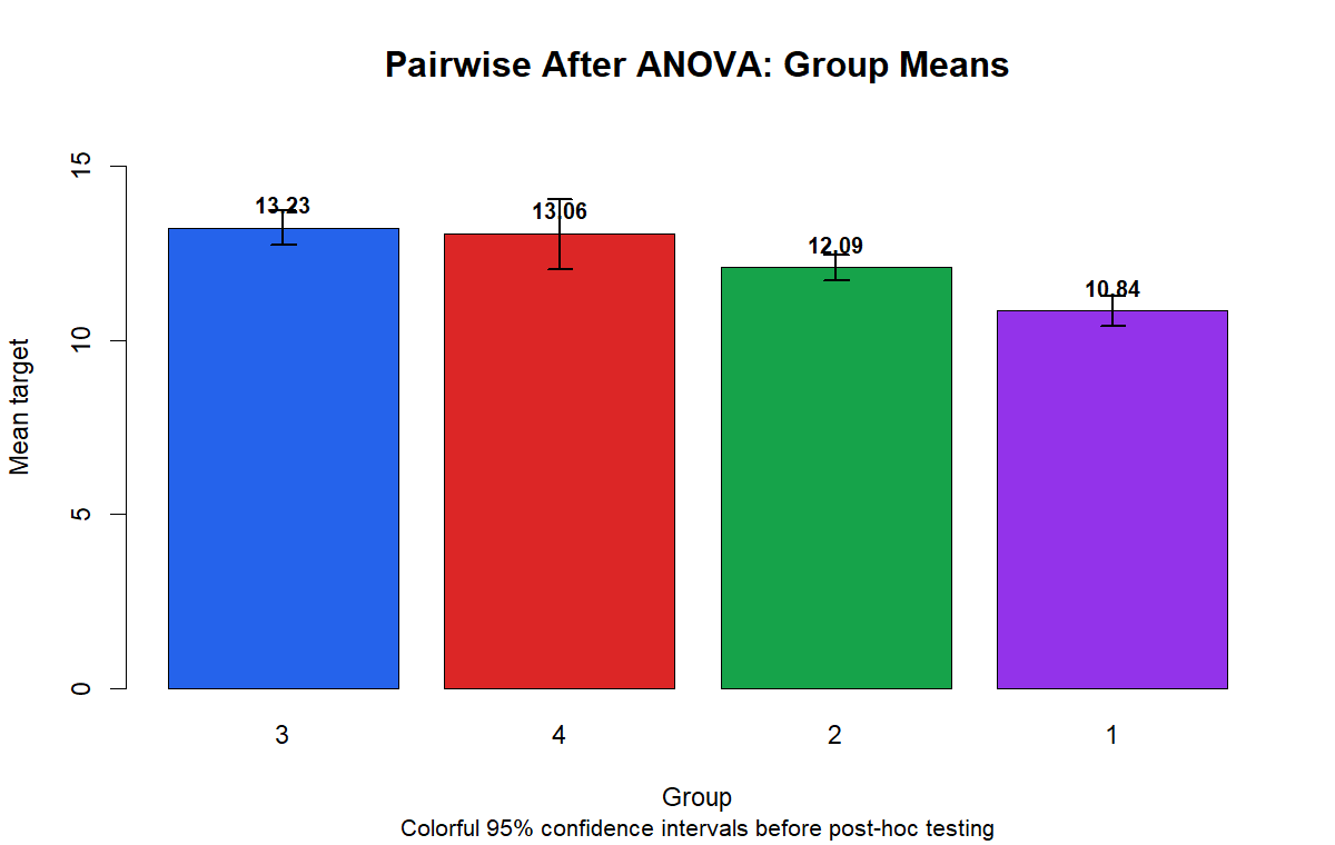
The group means chart shows the practical reason for post hoc testing. Group 1 has the lowest average G3 score, group 2 is higher, and groups 3 and 4 have the highest means. This pattern explains why the overall ANOVA was significant.
The confidence intervals show uncertainty around each group mean. The smallest group has a wider interval, so its mean should be interpreted with sample-size context. Pairwise comparisons convert these visible differences into adjusted statistical decisions.
Python Chart 2: Group Distribution Boxplots
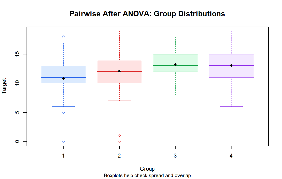
The boxplots show how G3 scores are distributed within each studytime group. Group 1 is centered lower than the other groups, while groups 3 and 4 are centered higher. This supports the same mean pattern shown in the confidence interval chart.
The chart also shows that group distributions overlap. This is why statistical testing is needed. Overlap does not automatically mean no difference; the test compares mean differences relative to sample size and within-group variation.
Python Chart 3: ANOVA Sum of Squares Breakdown
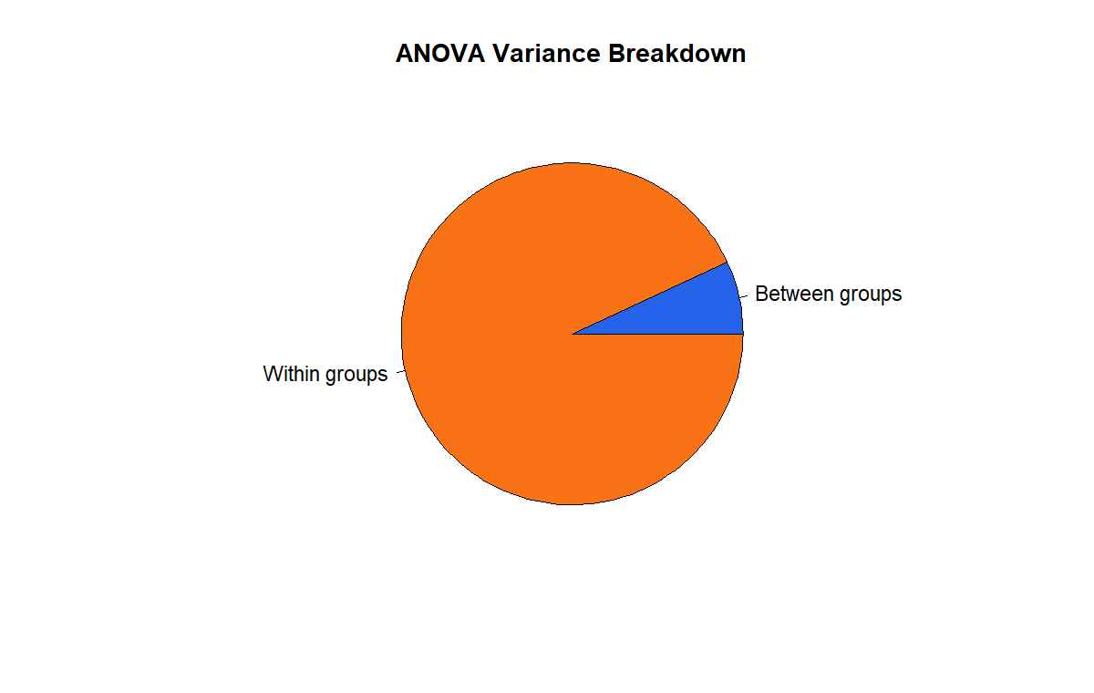
The sum of squares chart explains the overall ANOVA result. Between-group variation represents differences among studytime group means. Within-group variation represents variation among students inside the same studytime groups.
The ANOVA becomes significant because the between-group mean square is large relative to the within-group mean square. Pairwise comparisons then identify which group means produce that overall difference.
Python Chart 4: Pairwise Adjusted p-values
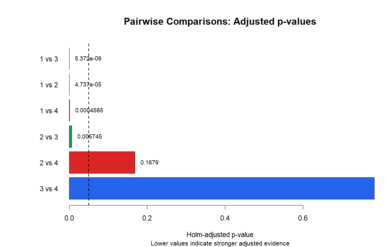
The adjusted p-value chart is the main post hoc decision chart. Pairs below the .05 line are interpreted as significant after correction. The strongest comparisons involve group 1 against the higher studytime groups and group 2 against group 3.
The chart also shows which comparisons should not be overstated. Groups 2 and 4 are closer, and groups 3 and 4 are very close. These pairs typically do not support strong adjusted significance claims.
Python Chart 5: Pairwise Mean Difference Heatmap
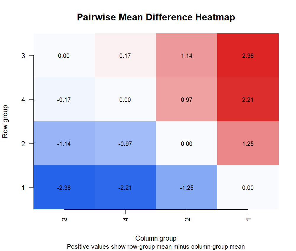
The mean difference heatmap shows the direction and size of group gaps. The biggest gap is between group 1 and group 3. Group 1 compared with group 4 is also large, and group 1 compared with group 2 is moderate.
The smallest gap is between group 3 and group 4. This explains why those two groups should be interpreted as similar unless a specific post hoc method says otherwise.
Python Chart 6: Adjustment Method Comparison
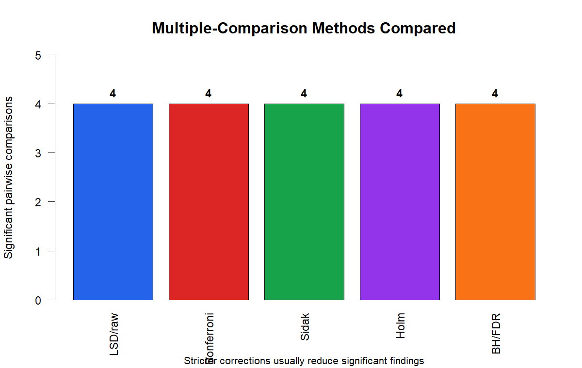
The adjustment method comparison chart shows why the selected post hoc method matters. Less conservative methods may mark more pairs as significant, while stricter methods may retain only the strongest differences.
This chart is useful for teaching because it shows that “significant” is not only about the raw mean difference. It also depends on the correction used to control false positives across multiple tests.
Python Chart 7: Group Size and Mean
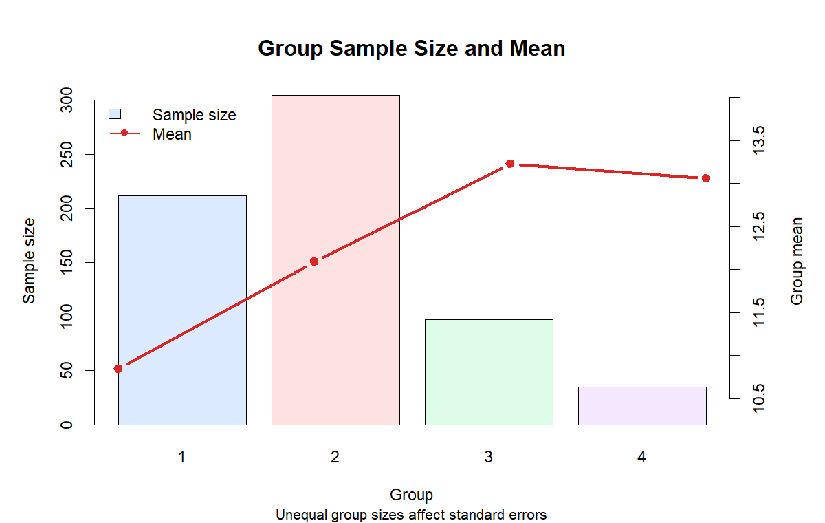
The group size and mean chart shows that group sizes are unequal. Group 2 is the largest, group 1 is also large, group 3 is smaller and group 4 is the smallest. This matters because smaller groups have less precise mean estimates.
Pairwise comparisons should therefore be interpreted with both mean size and sample size in mind. A high mean in a small group may still have a wider uncertainty interval.
Python Chart 8: Group Histograms
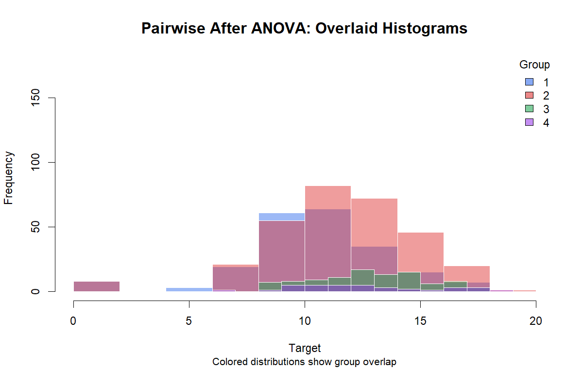
The histograms show the shape of G3 scores inside each studytime group. They help readers see whether group means summarize the data reasonably and whether some groups have unusual distribution patterns.
The histograms support a practical conclusion: the lowest studytime group contains more lower scores, while the higher studytime groups shift toward higher G3 values. This distribution context strengthens the pairwise interpretation.
R Chart-by-Chart Validation
The R charts validate the same pairwise comparison workflow using a separate analysis environment. The same group mean pattern, ANOVA interpretation, adjusted p-value logic and distribution context appear again.
R Chart 1: Group Means with Confidence Intervals
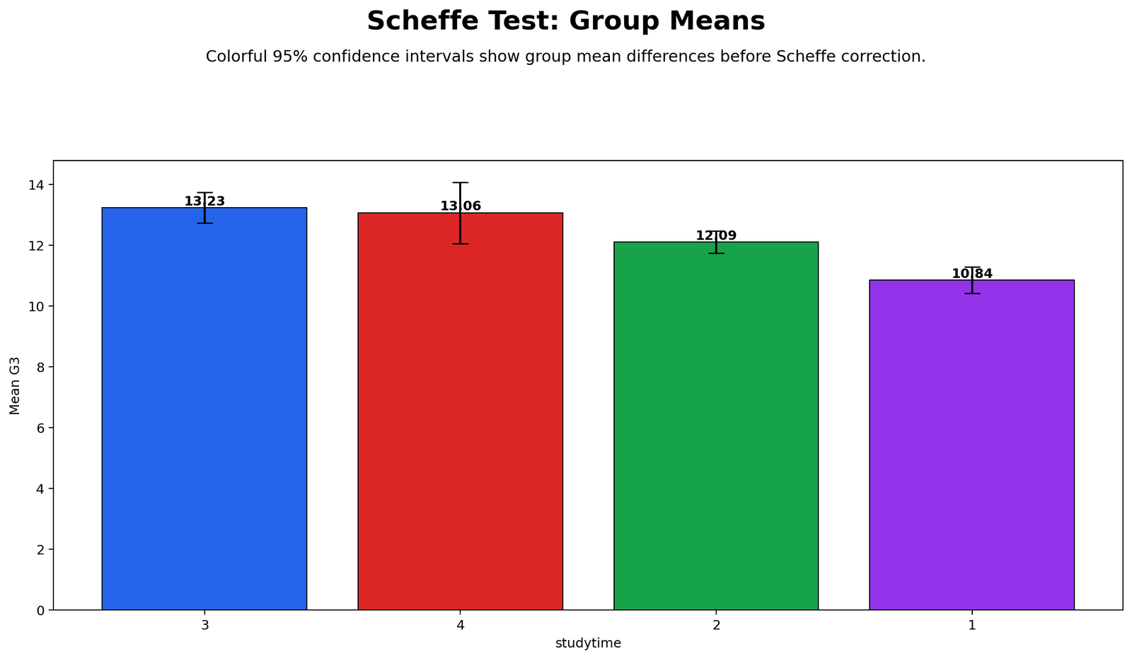
The R group means chart confirms the Python pattern. Group 1 is the lowest group, group 2 is higher, and groups 3 and 4 have the highest means. This software-to-software agreement supports the final interpretation.
The chart also reinforces that groups 3 and 4 are close. Their small mean difference should be treated carefully in the final report.
R Chart 2: Group Distribution Boxplots
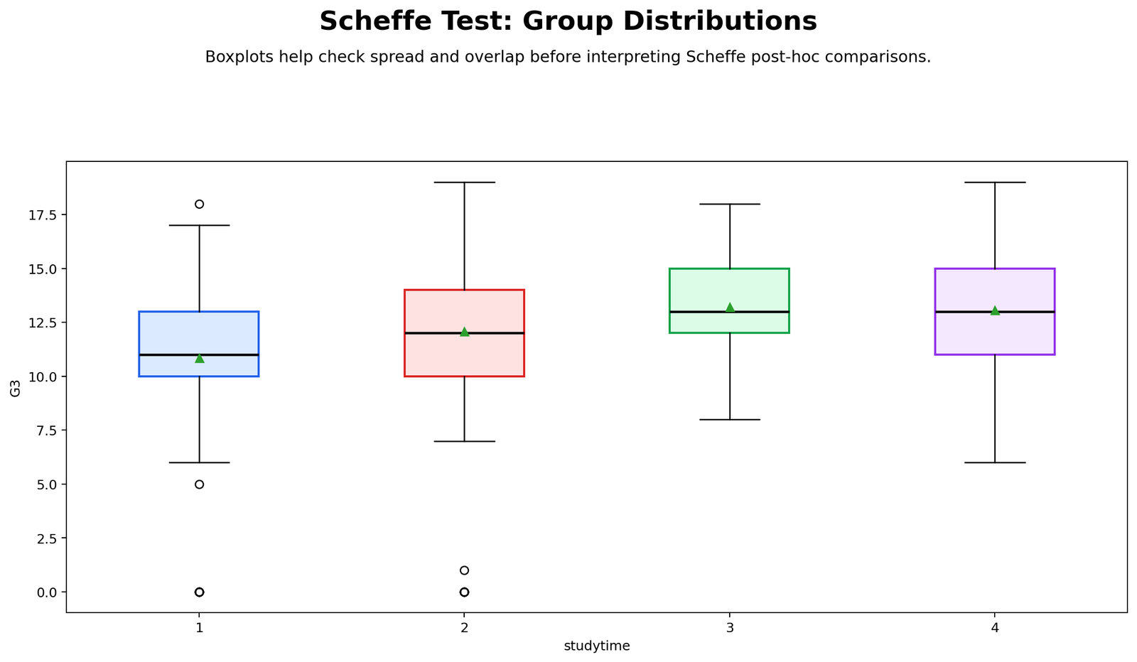
The R boxplots validate the distribution pattern. Group 1 has a lower center, while higher studytime groups are shifted upward.
This distribution view helps readers understand why pairwise comparisons involving group 1 are the strongest. It also shows that group overlap remains, which is normal in real data.
R Chart 3: ANOVA Sum of Squares Breakdown
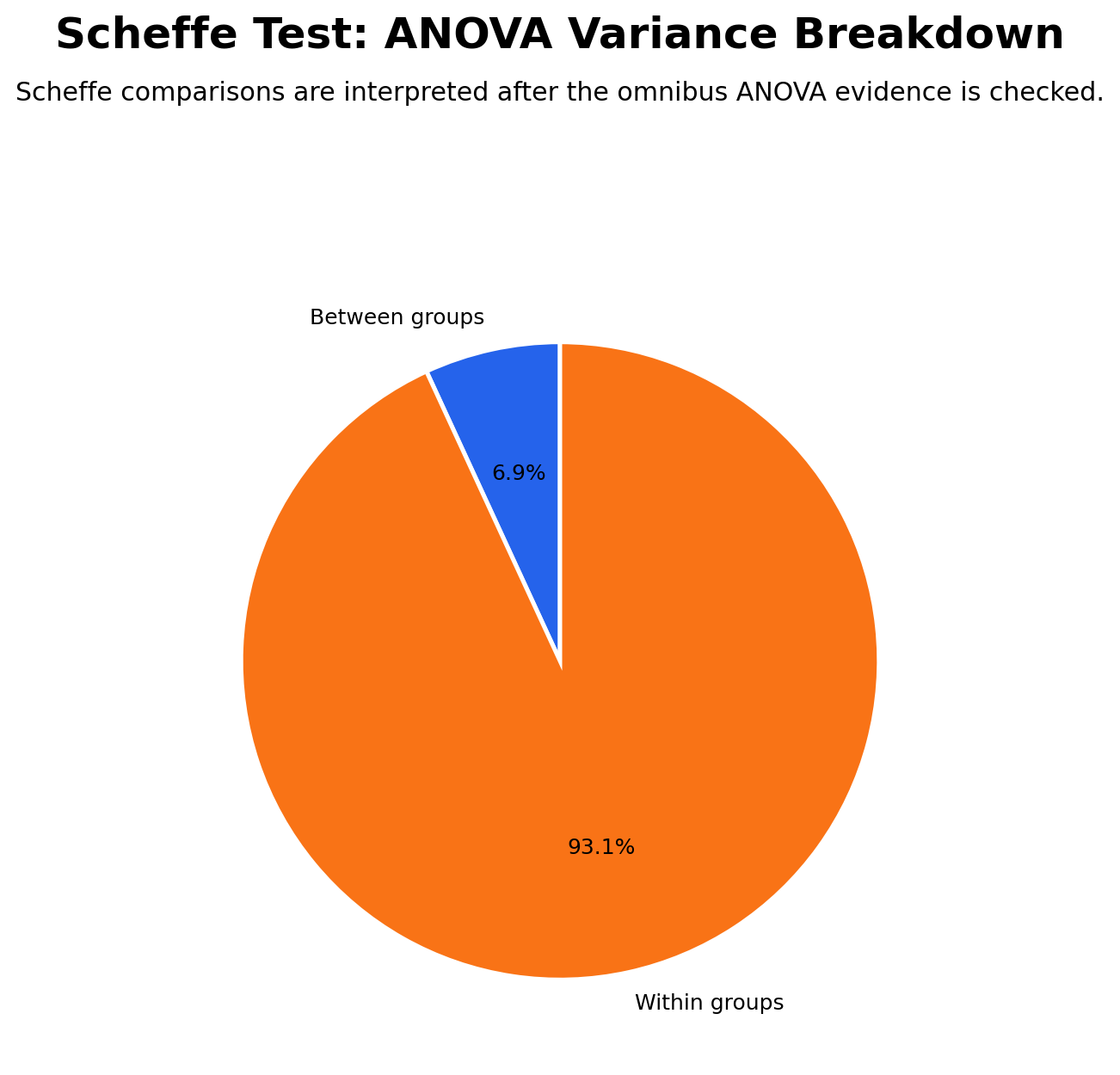
The R sum of squares chart confirms the same ANOVA logic. Between-group variation is large enough compared with within-group variation to justify post hoc interpretation.
This chart connects the ANOVA table to the pairwise tests. The post hoc comparisons are not separate from ANOVA; they explain the overall ANOVA result.
R Chart 4: Pairwise Adjusted p-values
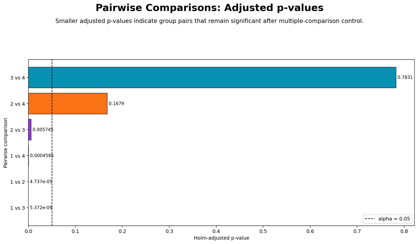
The R adjusted p-value chart validates the same decision pattern. The strongest comparisons are those involving group 1 and the higher studytime groups.
The weaker comparisons, especially between groups 3 and 4, should not be described as strong differences. This keeps the report accurate and prevents overclaiming.
R Chart 5: Pairwise Mean Difference Heatmap
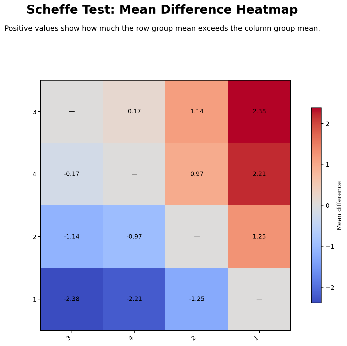
The R heatmap confirms the same mean difference structure. The largest difference is between the lowest and highest mean groups, while groups 3 and 4 remain very close.
The heatmap is useful because it shows direction and size, not just statistical significance. Pairwise reporting should always include mean difference interpretation.
R Chart 6: Adjustment Method Comparison
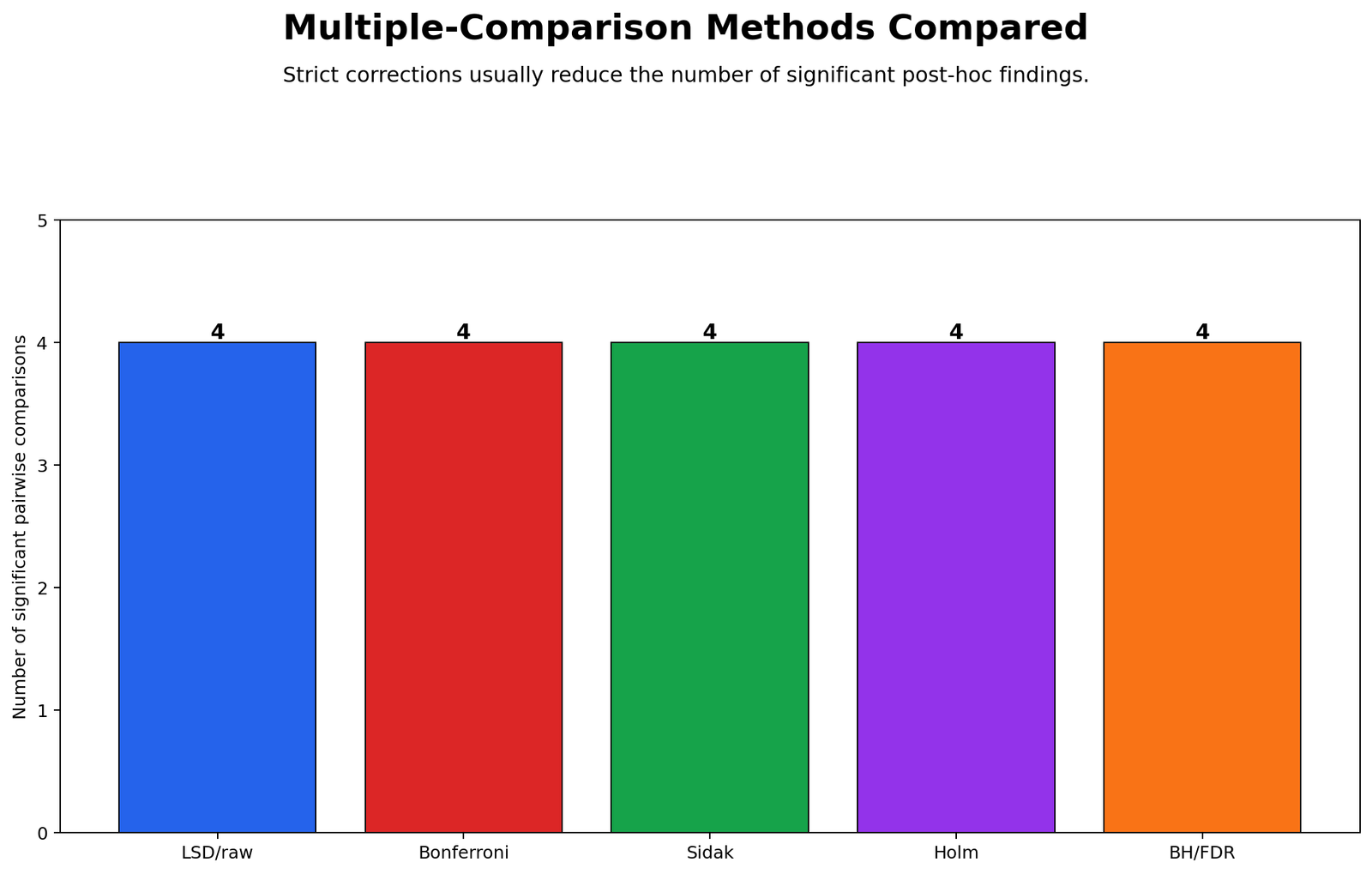
The R method comparison chart confirms that different correction methods can produce different levels of strictness. Holm and Tukey-style methods usually protect against false positives more than unadjusted p-values.
This chart supports the best reporting practice: always name the adjustment method. A sentence that says “pairwise comparisons were significant” is incomplete unless the correction method is stated.
R Chart 7: Group Size and Mean
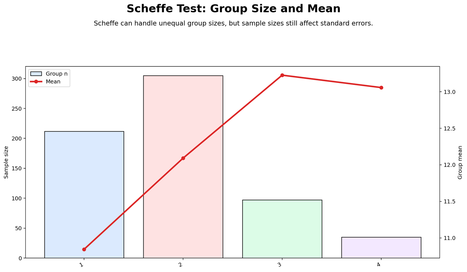
The R group size chart confirms the unequal sample-size structure. Group 4 has the smallest sample size, so comparisons involving group 4 should be read with more uncertainty.
This chart explains why a mean difference can look visible but still fail to become significant after adjustment. Sample size and variability both affect the final decision.
R Chart 8: Group Histograms
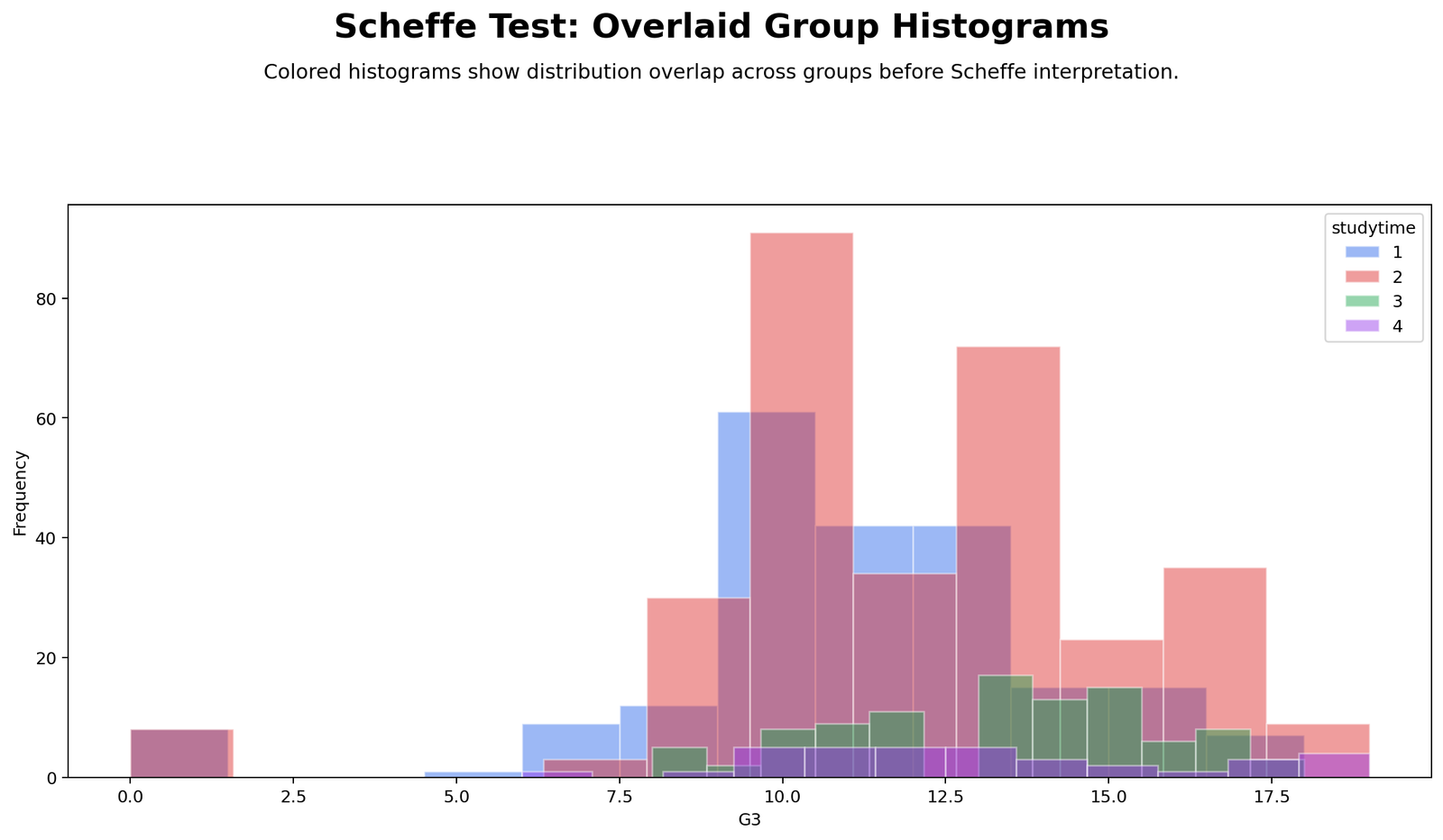
The R histograms confirm that group distributions differ in center and spread. The lowest studytime group contains more lower scores, while higher studytime groups shift upward.
This final validation chart supports the whole post hoc story. The ANOVA shows an overall difference, the pairwise tests identify the group pairs, and the histograms show the raw distribution context behind the results.
SPSS, R, Python and Excel Workflows for Pairwise Comparisons After ANOVA
Pairwise comparisons after ANOVA can be completed in SPSS, R, Python and Excel. SPSS is easiest for menu-based post hoc tests. R and Python are best for reproducible adjusted p-values and custom charts. Excel is useful for teaching the formulas but is weaker for full post hoc automation.
SPSS Workflow
| Step | SPSS Action | Purpose |
|---|---|---|
| Open data | File > Open > Data | Load the cleaned dataset containing G3 and studytime. |
| Run ANOVA | Analyze > Compare Means > One-Way ANOVA | Set G3 as dependent variable and studytime as factor. |
| Check assumptions | Options > Descriptive and Homogeneity of variance test | Review group means, standard deviations and Levene test. |
| Select post hoc method | Post Hoc > Tukey, Bonferroni, Gabriel, Games-Howell or others | Choose the method based on assumptions and group sizes. |
| Interpret output | Read Multiple Comparisons table | Report mean differences, adjusted p-values and confidence intervals. |
R Workflow
| Step | R Action | Purpose |
|---|---|---|
| Read data | read.csv() | Import the dataset. |
| Fit ANOVA | aov(G3 ~ factor(studytime)) | Run one-way ANOVA. |
| Run pairwise tests | pairwise.t.test() or TukeyHSD() | Calculate pairwise comparisons. |
| Adjust p-values | p.adjust.method = "holm", "bonferroni" or Tukey output | Control multiple-comparison error. |
Python Workflow
| Step | Python Action | Purpose |
|---|---|---|
| Read data | pandas.read_csv() | Load G3 and studytime variables. |
| Fit ANOVA | statsmodels.formula.api.ols() | Estimate the one-way ANOVA model. |
| Run Tukey HSD | pairwise_tukeyhsd() | Get adjusted pairwise comparisons. |
| Run custom comparisons | multipletests() | Compare adjustment methods such as Bonferroni and Holm. |
Excel Workflow
Excel can run the ANOVA through the Analysis ToolPak and can calculate mean differences and simple pairwise t tests manually. However, Excel does not provide a complete post hoc comparison system as easily as SPSS, R or Python.
| Excel Item | Formula Idea | Purpose |
|---|---|---|
| Group mean | =AVERAGEIF(group_range, group_id, value_range) | Calculate each group mean. |
| Group sample size | =COUNTIF(group_range, group_id) | Count observations in each group. |
| Mean difference | =mean_i-mean_j | Calculate pairwise difference. |
| Standard error | =SQRT(MSE*(1/n_i+1/n_j)) | Calculate pairwise uncertainty. |
| Bonferroni threshold | =0.05/number_of_comparisons | Apply a simple multiple-comparison correction. |
Code Blocks for Pairwise Comparisons After ANOVA
SPSS Syntax
ONEWAY G3 BY studytime
  /STATISTICS DESCRIPTIVES HOMOGENEITY
  /POSTHOC = TUKEY BONFERRONI ALPHA(0.05).
R Code
data <- read.csv("dataset.csv")
data$studytime <- factor(data$studytime)

# One-way ANOVA

model <- aov(G3 ~ studytime, data = data)
summary(model)

# Tukey pairwise comparisons

TukeyHSD(model)

# Holm adjusted pairwise t tests

pairwise.t.test(
x = data$G3,
g = data$studytime,
p.adjust.method = "holm",
pool.sd = TRUE
)
Python Code
import pandas as pd
import itertools
from scipy import stats
import statsmodels.api as sm
import statsmodels.formula.api as smf
from statsmodels.stats.multicomp import pairwise_tukeyhsd
from statsmodels.stats.multitest import multipletests

df = pd.read_csv("dataset.csv")
df["studytime"] = df["studytime"].astype("category")

# One-way ANOVA

model = smf.ols("G3 ~ C(studytime)", data=df).fit()
anova = sm.stats.anova_lm(model, typ=2)
print(anova)

# Tukey HSD

tukey = pairwise_tukeyhsd(
endog=df["G3"],
groups=df["studytime"],
alpha=0.05
)
print(tukey)

# Pairwise t tests with Holm correction

summary = df.groupby("studytime")["G3"].agg(["count", "mean", "std", "var"])

rows = []
for g1, g2 in itertools.combinations(summary.index, 2):
x1 = df.loc[df["studytime"] == g1, "G3"]
x2 = df.loc[df["studytime"] == g2, "G3"]
t_stat, p_value = stats.ttest_ind(x1, x2, equal_var=True)
rows.append([g1, g2, x1.mean() - x2.mean(), t_stat, p_value])

pairwise = pd.DataFrame(rows, columns=[
"group_1", "group_2", "mean_difference", "t_statistic", "p_unadjusted"
])

reject, p_holm, _, _ = multipletests(pairwise["p_unadjusted"], method="holm")
pairwise["p_holm_adjusted"] = p_holm
pairwise["significant_holm"] = reject

print(pairwise)
Excel Formula Pattern
Group mean:
=AVERAGEIF(group_range, group_id, value_range)

Group sample size:
=COUNTIF(group_range, group_id)

Mean difference:
=Mean_Group_i - Mean_Group_j

Pairwise standard error:
=SQRT(MSE*(1/n_i + 1/n_j))

Pairwise t value:
=Mean_Difference/Standard_Error

Two-tailed p-value:
=T.DIST.2T(ABS(t_value), df_error)

Bonferroni adjusted p-value:
=MIN(unadjusted_p*number_of_comparisons, 1)

Decision:
=IF(adjusted_p<0.05,"Significant","Not significant")
APA Reporting Wording for Pairwise Comparisons After ANOVA
A one-way ANOVA was conducted to compare G3 final grade across four studytime groups. The ANOVA was statistically significant, indicating that mean final grade differed across studytime levels. Pairwise comparisons were then conducted using adjusted p-values to identify which groups differed.
The pairwise results showed that the lowest studytime group had lower mean G3 scores than several higher studytime groups. The largest difference was between group 1 and group 3. The difference between groups 3 and 4 was small and should not be interpreted as a strong post hoc difference unless the adjusted comparison table supports that decision.
Short APA version: A one-way ANOVA showed a significant effect of studytime on G3. Adjusted pairwise comparisons showed that group 1 had lower G3 scores than the higher studytime groups, while the highest two groups were not clearly separated.
Common Mistakes in Pairwise Comparisons After ANOVA
| Mistake | Why It Is a Problem | Better Practice |
|---|---|---|
| Reporting only the ANOVA p-value | The ANOVA does not identify which groups differ. | Report adjusted pairwise comparisons after a significant ANOVA. |
| Using unadjusted p-values for many tests | Multiple testing increases false-positive risk. | Use Tukey, Bonferroni, Holm or another correction method. |
| Not naming the adjustment method | Different methods can lead to different decisions. | State the correction method clearly. |
| Ignoring mean differences | P-values do not show direction or practical size. | Report group means and mean differences. |
| Claiming all groups differ | Some pairs are close and may not be significant after adjustment. | Report each pair accurately. |
Most important warning: Do not say “all studytime groups are different” unless every adjusted pairwise comparison is significant. In this example, the safest interpretation is that group 1 is the main low group and groups 3 and 4 are close.
Downloads and Resources
Use the following downloadable outputs to verify the Pairwise Comparisons After ANOVA result and compare the Python and R workflows.
FAQs About Pairwise Comparisons After ANOVA
What are pairwise comparisons after ANOVA?
Pairwise comparisons after ANOVA are post hoc tests that compare group means two at a time after the overall ANOVA shows that at least one group mean differs.
Why are pairwise comparisons needed after ANOVA?
ANOVA tells whether not all group means are equal, but it does not identify the exact groups that differ. Pairwise comparisons identify those specific group differences.
How many pairwise comparisons are there for four groups?
There are six pairwise comparisons for four groups: 1 vs 2, 1 vs 3, 1 vs 4, 2 vs 3, 2 vs 4 and 3 vs 4.
Should I use adjusted p-values?
Yes. Because multiple tests are performed, adjusted p-values help control false-positive risk. Common methods include Tukey HSD, Bonferroni and Holm-Bonferroni.
What did this example show?
The example showed that group 1 had the lowest mean G3 score and group 3 had the highest. The strongest pairwise differences involved group 1 compared with higher studytime groups.
Can pairwise comparisons after ANOVA be done in Excel?
Yes, Excel can calculate group means, mean differences, t statistics and Bonferroni-adjusted p-values, but SPSS, R or Python is better for complete post hoc workflows.

