
Multiple Comparisons Correction, Holm Step-Down Procedure, Family-Wise Error Control
Holm Bonferroni Method: Formula, Interpretation, SPSS, Python, R and Excel Guide
Holm Bonferroni Method, also called the Holm-Bonferroni correction or Holm step-down procedure, is used to adjust multiple p-values while controlling the family-wise error rate. It is less conservative than the simple Bonferroni correction but still protects against false positives when many pairwise tests are performed. This guide explains the Holm Bonferroni Method with SPSS context, Python charts, R validation, Excel formulas, adjusted p-values, step-down decisions, APA reporting and downloadable resources.
Quick Answer: Holm Bonferroni Method Result
The worked example compares G3 final grade across four studytime groups. The sample contains 649 students. The one-way ANOVA was statistically significant, F(3, 645) = 15.876, p < .001, so pairwise follow-up tests were justified. The Holm Bonferroni Method was then applied to the six pairwise p-values to control family-wise error.
The group means increased from the lowest studytime group to the higher studytime groups. Group 1 had the lowest mean G3 score, M = 10.84. Group 2 had M = 12.09. Group 4 had M = 13.06. Group 3 had the highest mean, M = 13.23. After Holm adjustment, 4 pairwise comparisons remained significant out of 6 total comparisons.
Final interpretation: The Holm Bonferroni Method shows that studytime group 1 differs significantly from groups 2, 3 and 4. Group 2 also differs significantly from group 3. The comparisons 2 vs 4 and 3 vs 4 are not statistically significant after Holm adjustment. In plain language, the lowest studytime group had lower final grades than the higher studytime groups, while the highest studytime categories were not clearly different from each other.
Important reporting point: Holm-Bonferroni is not a separate ANOVA model. It is a p-value adjustment method. First calculate the pairwise p-values, then sort them from smallest to largest, then apply the Holm step-down rule.
Table of Contents
- What Is Holm Bonferroni Method?
- When to Use Holm Bonferroni Method
- Holm Bonferroni Method Formula
- Null and Alternative Hypotheses
- Dataset and Variables Used
- SPSS Output Interpretation
- Python Chart-by-Chart Interpretation
- R Chart-by-Chart Validation
- SPSS, R, Python and Excel Workflows
- Code Blocks for Holm Bonferroni Method
- APA Reporting Wording
- Common Mistakes
- Downloads and Resources
- Related Guides
- FAQs
What Is Holm Bonferroni Method?
Holm Bonferroni Method is a multiple comparison correction used when a researcher tests several hypotheses at the same time. Without adjustment, testing many pairwise p-values increases the chance of getting at least one false-positive result. Holm-Bonferroni controls this family-wise error problem while keeping more statistical power than the classic Bonferroni correction.
The method works by ordering p-values from smallest to largest. The smallest p-value is tested against the strictest threshold. If it passes, the next smallest p-value is tested against a slightly less strict threshold. This continues until a p-value fails. After the first failure, the remaining larger p-values are not rejected.
In post hoc analysis, Holm Bonferroni Method is commonly used after an ANOVA or after a planned set of pairwise t tests. It is flexible because it can adjust any list of p-values, whether they came from pairwise t tests, correlation tests, regression contrasts or other multiple testing situations.
Simple definition: Holm Bonferroni Method is a step-down p-value correction that controls family-wise error by testing the smallest p-values first and using progressively less strict thresholds.
Before using this method, review one-way ANOVA, p-values, null and alternative hypothesis, confidence intervals, and Type I and Type II error.
When to Use Holm Bonferroni Method
Use Holm Bonferroni Method when you have several p-values and you want to control the family-wise error rate. In this guide, the method is used after one-way ANOVA to adjust six pairwise comparisons among four studytime groups.
| Use Holm Bonferroni When | Why It Matters | Example in This Guide |
|---|---|---|
| You test multiple pairwise comparisons | Multiple testing increases the chance of false positives. | Four studytime groups create six pairwise tests. |
| You want stronger control than unadjusted p-values | Unadjusted p-values can overstate significance when many tests are run. | Unadjusted p-values were corrected using Holm adjustment. |
| You want more power than simple Bonferroni | Holm-Bonferroni is usually less conservative than applying α/m to every test. | Four comparisons remained significant after adjustment. |
| You have planned or post hoc hypotheses | The method can adjust a family of p-values from many sources. | Pairwise pooled t tests after ANOVA were adjusted. |
When not to use it alone: Holm-Bonferroni adjusts p-values, but it does not replace assumption checking. For ANOVA pairwise comparisons, still review group distributions, variance context, sample sizes and the logic of the original pairwise tests.
Holm Bonferroni Method Formula
Suppose there are m p-values in one family of tests. First sort the p-values from smallest to largest:
The Holm step-down threshold for the kth ordered p-value is:
The decision rule is:
For adjusted p-values, the Holm adjusted value is calculated in sorted order by multiplying each p-value by the number of remaining tests and applying a cumulative maximum:
| Symbol | Meaning | Interpretation |
|---|---|---|
| m | Number of tests | Six pairwise tests in this example. |
| p(k) | kth smallest p-value | The p-value being tested at step k. |
| α | Overall significance level | Usually .05. |
| α/(m-k+1) | Holm step-down threshold | The cutoff used for the kth ordered p-value. |
| pHolm | Holm adjusted p-value | The p-value after family-wise error correction. |
Holm Step-Down Decisions in This Example
| Step | Comparison | Unadjusted p | Holm Threshold | Holm Adjusted p | Decision |
|---|---|---|---|---|---|
| 1 | 1 vs 3 | 8.952930e-10 | .00833 | 5.371758e-09 | Reject equal means |
| 2 | 1 vs 2 | 9.473280e-06 | .01000 | 4.736640e-05 | Reject equal means |
| 3 | 1 vs 4 | 1.146236e-04 | .01250 | 4.584943e-04 | Reject equal means |
| 4 | 2 vs 3 | .001914916 | .01667 | .005744748 | Reject equal means |
| 5 | 2 vs 4 | .08393031 | .02500 | .1678606 | Fail to reject equal means |
| 6 | 3 vs 4 | .7831343 | .05000 | .7831343 | Fail to reject equal means |
Null and Alternative Hypotheses for Holm Bonferroni Method
The Holm Bonferroni Method is applied to a family of individual hypotheses. Each pairwise comparison has a null and alternative hypothesis, and Holm adjusts the decision so the whole family of tests is protected.
| Pairwise Test | Hypothesis | Meaning |
|---|---|---|
| Null hypothesis | H0: μi = μj | The two studytime groups have equal mean G3 scores. |
| Alternative hypothesis | H1: μi ≠ μj | The two studytime groups have different mean G3 scores. |
| Family-wise decision | Holm adjusted p < .05 | The pair remains significant after multiple-comparison correction. |
Decision for this example: Holm adjustment rejected equal means for 1 vs 3, 1 vs 2, 1 vs 4, and 2 vs 3. It failed to reject equal means for 2 vs 4 and 3 vs 4.
Dataset and Variables Used
The worked example uses a student performance dataset. The dependent variable is G3 final grade. The grouping variable is studytime, coded into four weekly study-time groups. The analysis asks whether average final grade differs across studytime groups and which pairwise differences remain significant after Holm correction.
| Variable | Role | How It Is Used in Holm Bonferroni Method |
|---|---|---|
| G3 | Dependent variable | The final grade score being compared across groups. |
| studytime | Grouping factor | The four-level factor used to create six pairwise tests. |
| Group 1 | < 2 hours | Lowest studytime group and lowest mean G3 score. |
| Group 2 | 2 to 5 hours | Middle studytime group with higher mean than group 1. |
| Group 3 | 5 to 10 hours | Highest mean G3 score in this example. |
| Group 4 | > 10 hours | High mean G3 score but not significantly different from groups 2 or 3 after Holm correction. |
Before interpreting Holm-adjusted p-values, review the group means, distributions and variance context. Helpful related guides include descriptive statistics, box plot interpretation, Levene test, and ANOVA in SPSS.
SPSS Output Interpretation for Holm Bonferroni Method
The SPSS output confirms the ANOVA context and gives a Bonferroni comparison table for reference. SPSS one-way ANOVA menus do not always provide a direct Holm-Bonferroni post hoc option in the same way that Python and R can adjust p-values directly. Therefore, the correct workflow is to use SPSS for group descriptives, assumption context and ANOVA, then apply Holm adjustment to the pairwise p-values in Python, R or Excel.
SPSS Group Descriptives
| Studytime Group | N | Mean G3 | Std. Deviation | Variance | Minimum | Maximum | Interpretation |
|---|---|---|---|---|---|---|---|
| 1 | 212 | 10.84 | 3.219 | 10.360 | 0 | 18 | Lowest average final grade. |
| 2 | 305 | 12.09 | 3.243 | 10.518 | 0 | 19 | Higher than group 1. |
| 3 | 97 | 13.23 | 2.502 | 6.261 | 8 | 18 | Highest average final grade. |
| 4 | 35 | 13.06 | 3.038 | 9.232 | 6 | 19 | High mean but smallest group size. |
| Total | 649 | 11.91 | 3.231 | 10.437 | 0 | 19 | Overall final grade mean. |
SPSS Homogeneity of Variances
| Test | Statistic | df1 | df2 | p-value | Interpretation |
|---|---|---|---|---|---|
| Levene test based on mean | 0.985 | 3 | 645 | .400 | Not significant; no strong equal-variance problem is indicated. |
| Levene test based on median | 1.026 | 3 | 645 | .380 | Also not significant. |
| Levene test based on trimmed mean | 1.081 | 3 | 645 | .356 | No strong variance warning from the trimmed mean version. |
SPSS One-Way ANOVA Table
| Source | Sum of Squares | df | Mean Square | F | Sig. | Interpretation |
|---|---|---|---|---|---|---|
| Between Groups | 465.078 | 3 | 155.026 | 15.876 | < .001 | At least one studytime group mean differs. |
| Within Groups | 6298.189 | 645 | 9.765 | Pooled error term for the ANOVA context. | ||
| Total | 6763.267 | 648 | Total variation in G3. |
Holm-Adjusted Pairwise Results
| Comparison | Mean Difference | Unadjusted p | Holm Adjusted p | Holm Decision | Plain Interpretation |
|---|---|---|---|---|---|
| 1 vs 3 | -2.382 | 8.952930e-10 | 5.371758e-09 | Significant | Group 1 scored significantly lower than group 3. |
| 1 vs 2 | -1.247 | 9.473280e-06 | 4.736640e-05 | Significant | Group 1 scored significantly lower than group 2. |
| 1 vs 4 | -2.213 | 1.146236e-04 | 4.584943e-04 | Significant | Group 1 scored significantly lower than group 4. |
| 2 vs 3 | -1.135 | .001914916 | .005744748 | Significant | Group 2 scored significantly lower than group 3. |
| 2 vs 4 | -0.965 | .08393031 | .1678606 | Not significant | Groups 2 and 4 do not differ clearly after Holm correction. |
| 3 vs 4 | 0.170 | .7831343 | .7831343 | Not significant | Groups 3 and 4 are statistically similar in this analysis. |
SPSS interpretation summary: SPSS confirms the group means, variance context and significant ANOVA. The exact Holm-Bonferroni decisions show four significant pairwise differences after p-value adjustment. The main difference pattern is that group 1 is lower than the higher studytime groups, while groups 3 and 4 are not significantly different.
Python Chart-by-Chart Interpretation
The Python charts show the full Holm Bonferroni workflow visually. They show group means, group distributions, unadjusted versus Holm-adjusted p-values, the step-down decision path, pairwise confidence intervals, a p-value heatmap and group standard deviation context.
Python Chart 1: Group Means with 95% Confidence Intervals
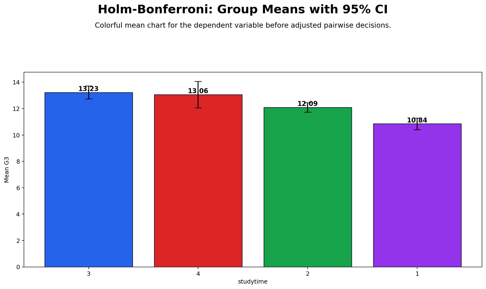
The group means chart shows that group 1 has the lowest mean G3 score, while groups 3 and 4 have the highest means. Group 2 sits between the lowest and highest categories. This visual pattern explains why the ANOVA was significant and why pairwise testing was useful.
The chart also shows that group 3 and group 4 have very close mean values. This explains why the Holm-adjusted comparison between groups 3 and 4 is not significant even though both groups are higher than group 1.
Python Chart 2: Group Distribution Boxplots
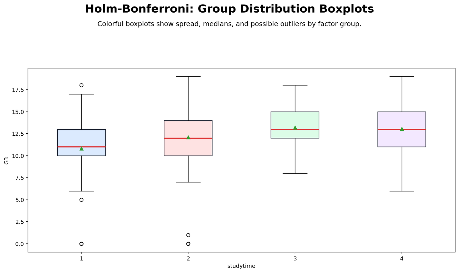
The boxplot shows the spread of G3 values inside each studytime group. Group 1 has the lowest central position and includes several very low scores. Groups 3 and 4 are centered higher, while group 2 is in the middle.
Holm-Bonferroni adjusts p-values, not distributions. The boxplot is therefore used as context. It helps readers understand why some pairs have strong evidence and why some high-studytime groups remain statistically similar.
Python Chart 3: Unadjusted vs Holm Adjusted p-values
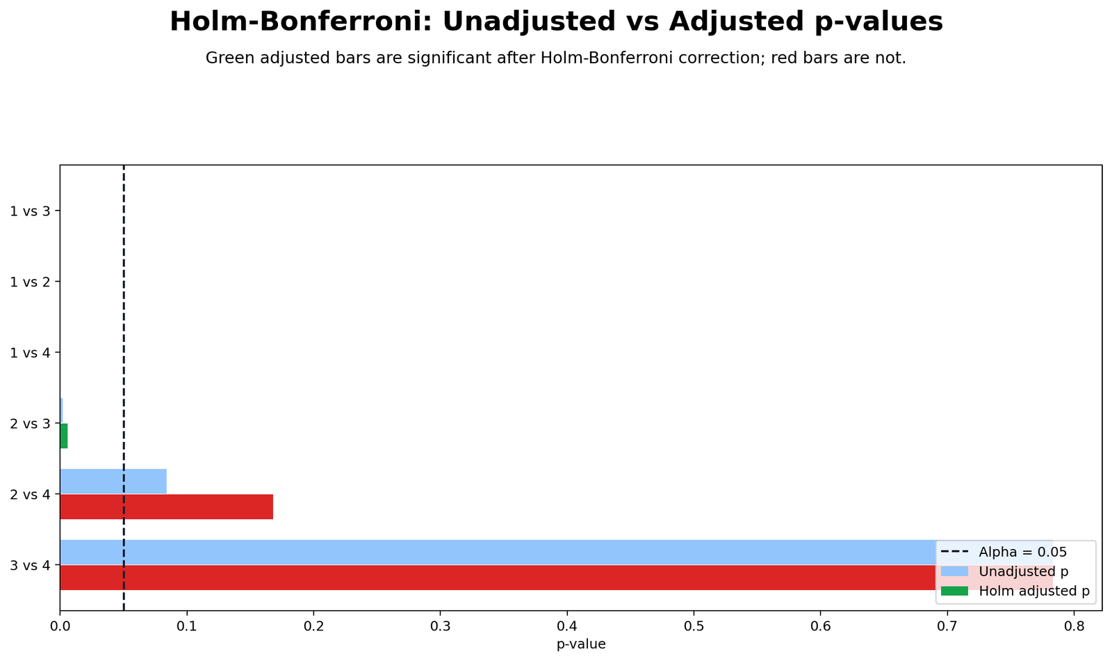
This chart shows how Holm correction changes the pairwise p-values. The smallest p-values remain very small after adjustment, so the comparisons 1 vs 3, 1 vs 2, 1 vs 4, and 2 vs 3 remain significant.
The comparison 2 vs 4 becomes clearly non-significant after adjustment, and 3 vs 4 is already far from significance. This chart is useful because it shows both the original evidence and the family-wise-error-controlled result.
Python Chart 4: Holm Step-Down Decision Path
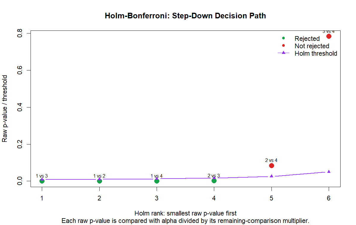
The step-down decision path shows the ordered p-values and the changing Holm thresholds. The first four p-values are smaller than their step-specific thresholds, so those four hypotheses are rejected. The fifth comparison, 2 vs 4, fails the Holm rule.
This chart is the core of the Holm Bonferroni Method. It shows why the method is not the same as applying one fixed Bonferroni threshold to every p-value. Holm starts strict and then becomes less strict as earlier tests are rejected.
Python Chart 5: Pairwise Mean Difference Confidence Intervals
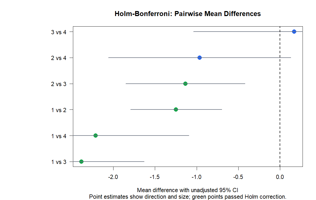
The mean difference chart uses zero as the no-difference reference line. Comparisons whose intervals stay away from zero are the strongest pairwise differences. In this example, the major differences involve group 1 compared with groups 2, 3 and 4, plus group 2 compared with group 3.
The intervals for 2 vs 4 and 3 vs 4 are consistent with non-significant Holm-adjusted decisions. These comparisons do not show a clear enough difference after accounting for multiple testing.
Python Chart 6: Holm Adjusted p-value Heatmap
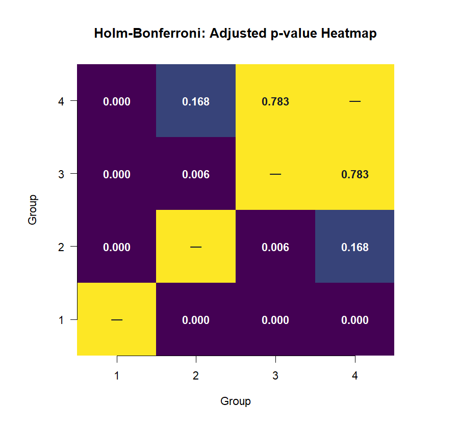
The heatmap gives a compact matrix view of Holm-adjusted pairwise decisions. It highlights that group 1 differs from groups 2, 3 and 4, and that group 2 differs from group 3.
The heatmap also makes the non-significant comparisons easy to see. Groups 2 and 4 do not differ clearly, and groups 3 and 4 are almost the same in mean G3 after adjustment.
Python Chart 7: Group Standard Deviation Context
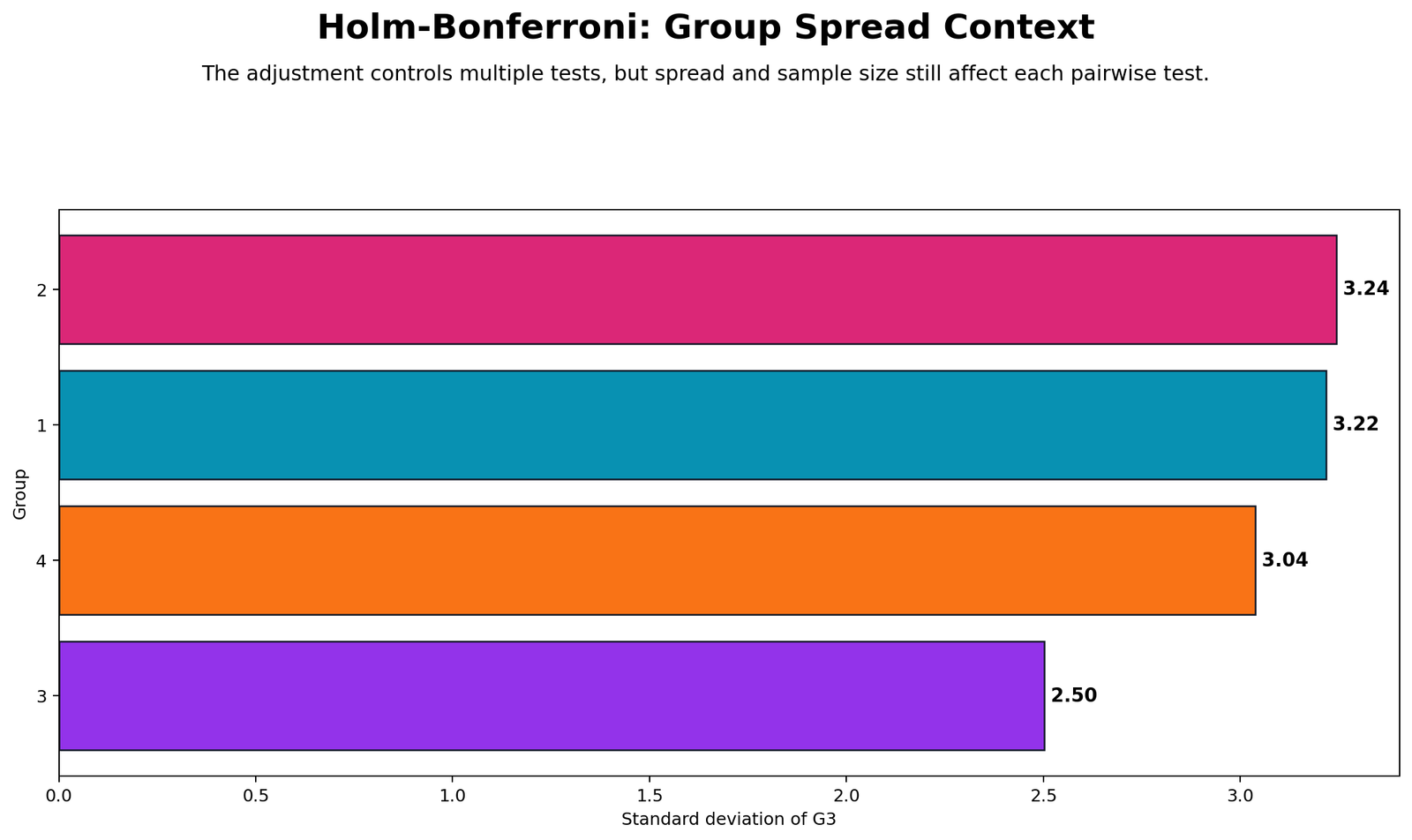
The standard deviation chart shows that group spread differs somewhat across the studytime groups. Group 3 has the smallest standard deviation, while groups 1 and 2 have larger standard deviations.
This chart does not change the Holm adjustment itself, but it improves interpretation. Pairwise tests depend on mean differences relative to uncertainty, so standard deviation context helps explain why some mean differences are significant and others are not.
R Chart-by-Chart Validation
The R validation charts confirm the Python result. The same group mean pattern appears, the same adjusted p-value decisions are reached, and the same four comparisons remain significant after Holm correction.
R Chart 1: Group Means with 95% Confidence Intervals
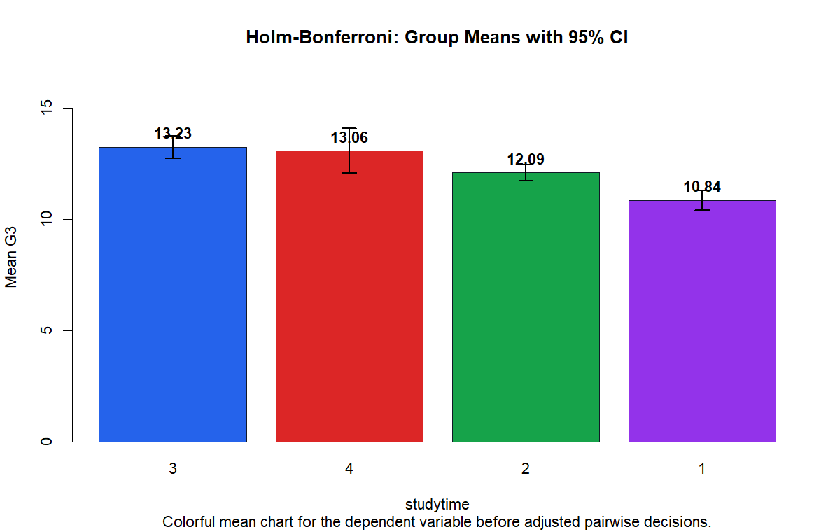
The R group means chart validates the same mean order: group 1 is lowest, group 2 is higher, and groups 3 and 4 are highest. This agreement supports the interpretation that the group mean pattern is stable across software.
The chart also reinforces that group 3 and group 4 are close together. This explains the non-significant adjusted result for the 3 vs 4 comparison.
R Chart 2: Group Distribution Boxplots
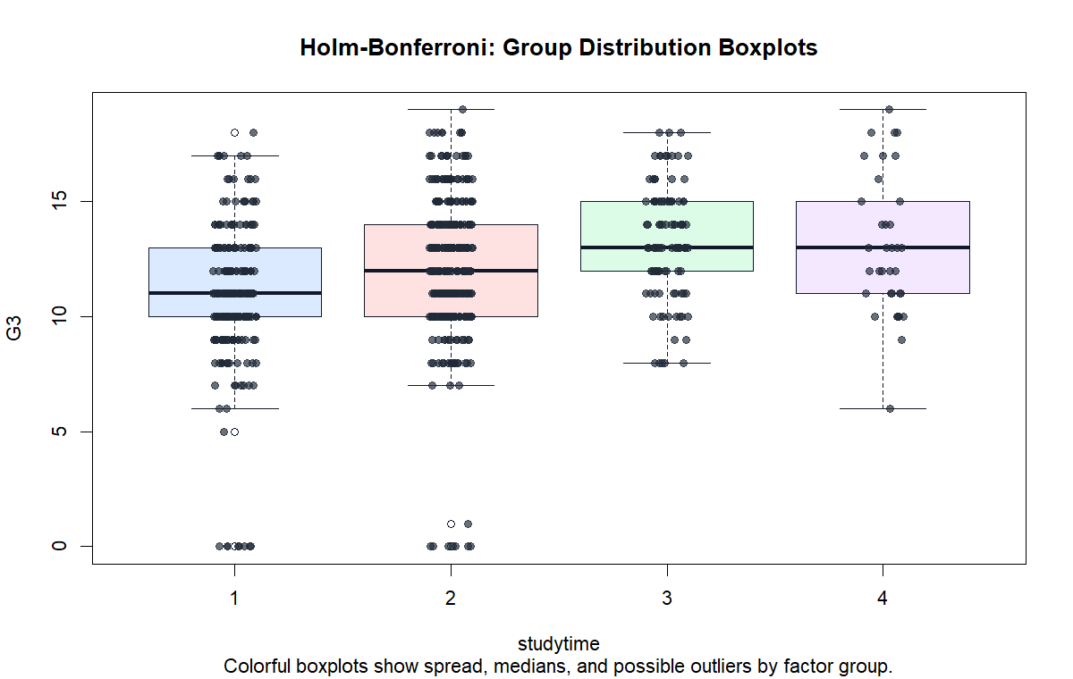
The R boxplot confirms the distribution pattern seen in Python. Group 1 is lower, groups 3 and 4 are higher, and group 2 sits in between.
This visual validation matters because Holm-Bonferroni decisions should be interpreted alongside the actual data structure. The plot shows that the significant p-values correspond to visible mean separation.
R Chart 3: Unadjusted vs Holm Adjusted p-values
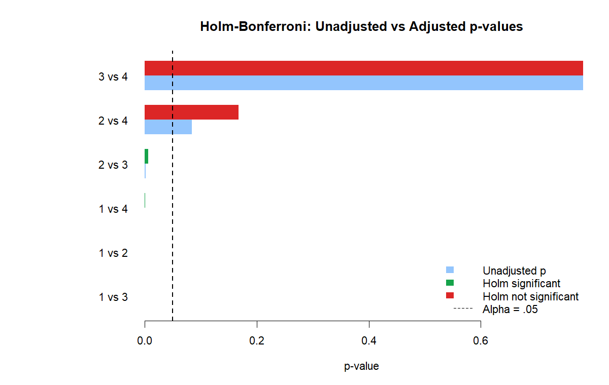
The R p-value chart confirms that the smallest four p-values remain below .05 after Holm adjustment. These are the comparisons involving group 1 and the comparison between group 2 and group 3.
The non-significant comparisons remain above the threshold after adjustment. This confirms that the result is not dependent on one software implementation.
R Chart 4: Holm Step-Down Decision Path
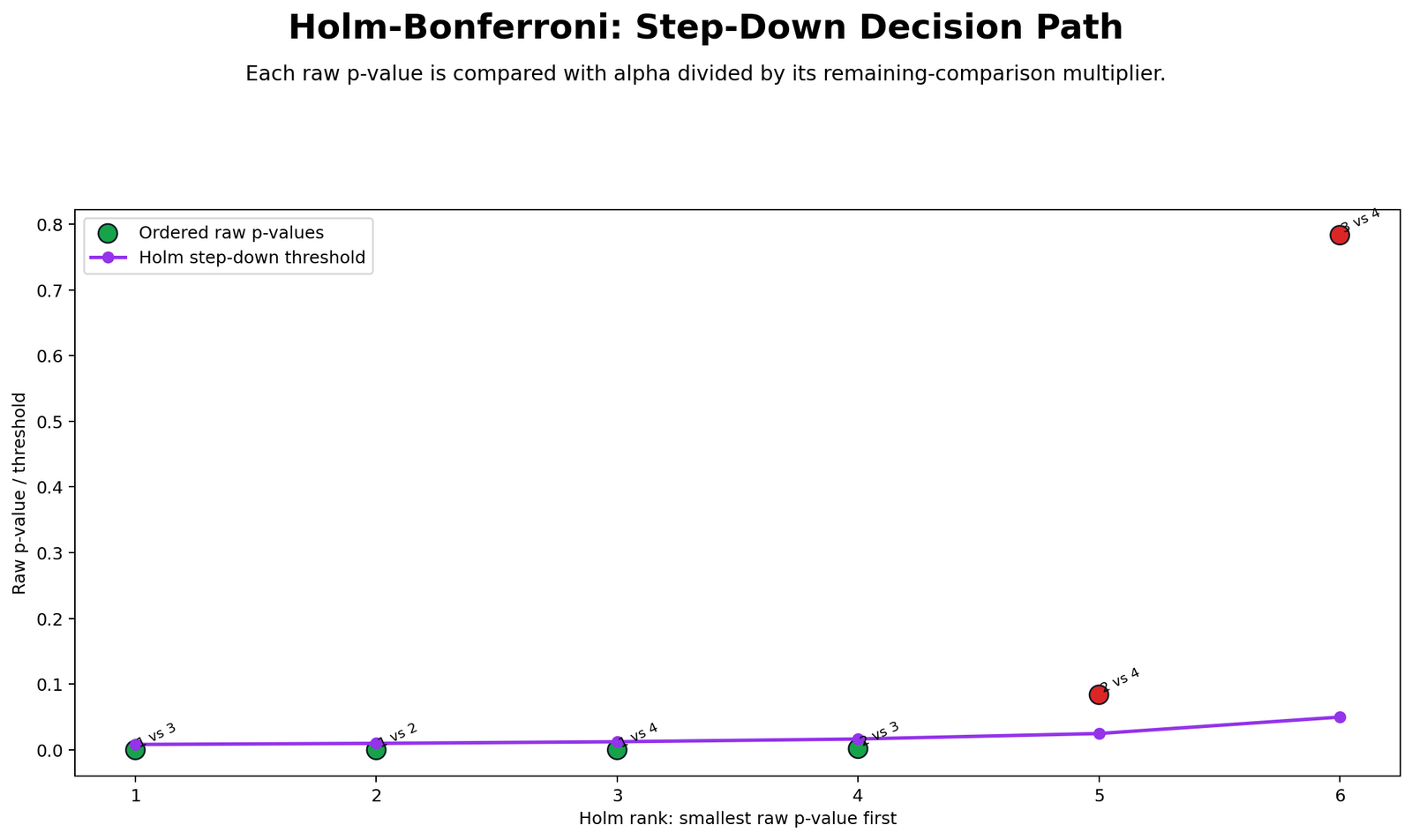
The R step-down chart validates the Holm procedure visually. The first four ordered p-values pass their Holm thresholds, while the fifth comparison does not. After the first failure, the remaining larger p-values are not rejected.
This chart is useful for teaching because it shows the exact reason the method is called a step-down procedure. It tests the strongest evidence first and stops rejecting when the evidence is no longer strong enough.
R Chart 5: Pairwise Mean Difference Confidence Intervals
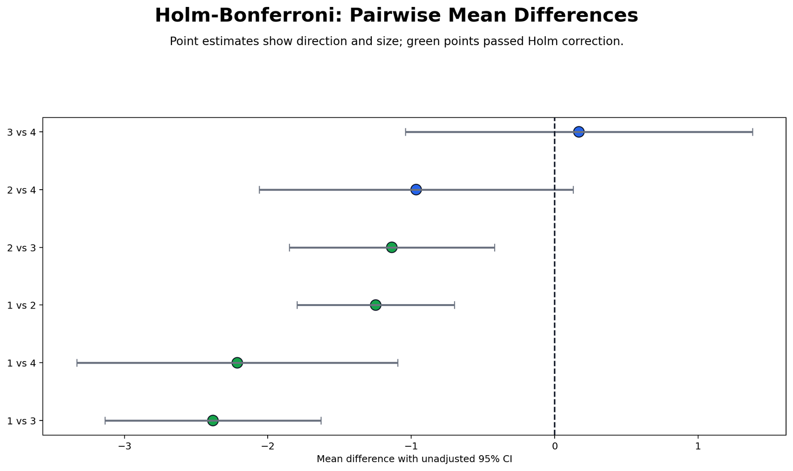
The R interval chart confirms the same direction of differences. Group 1 is lower than groups 2, 3 and 4, and group 2 is lower than group 3.
The comparisons between groups 2 and 4 and between groups 3 and 4 do not show a clear adjusted difference. This supports the final post hoc interpretation.
R Chart 6: Holm Adjusted p-value Heatmap
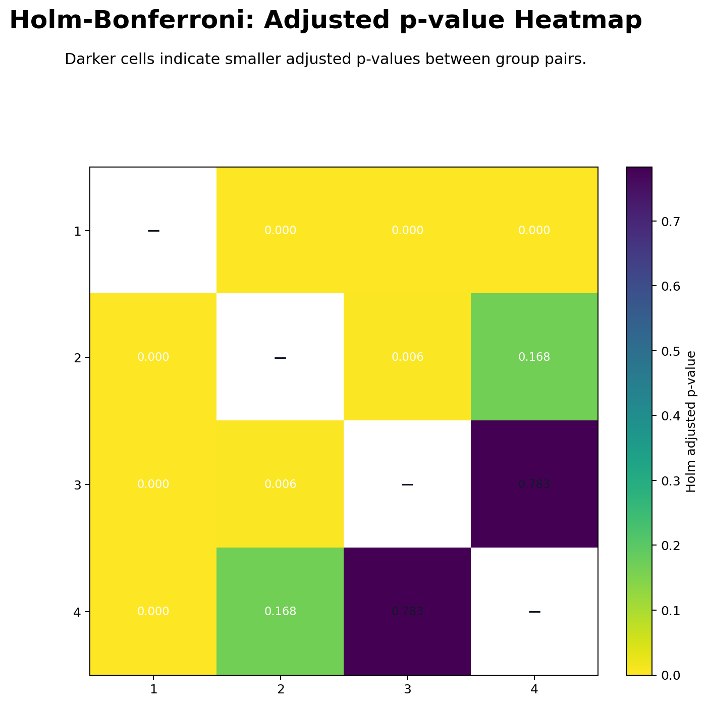
The R heatmap summarizes the adjusted p-values in a matrix format. It confirms that group 1 is the main separated group and that group 2 differs from group 3.
The non-significant cells for 2 vs 4 and 3 vs 4 support a careful report: the higher studytime groups are not all statistically different from one another.
R Chart 7: Group Standard Deviation Context
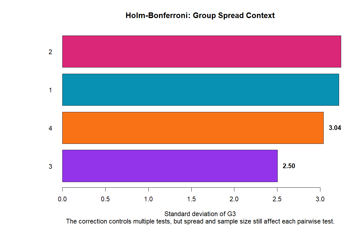
The R standard deviation chart confirms the spread pattern across groups. Group 3 is relatively tighter, while groups 1 and 2 show larger spread.
This validates the Python context chart and supports the overall interpretation that mean differences should be read together with uncertainty, not as raw differences alone.
SPSS, R, Python and Excel Workflows for Holm Bonferroni Method
The Holm Bonferroni Method can be reproduced in SPSS, R, Python and Excel. SPSS is useful for ANOVA and pairwise comparison context. R and Python can directly produce Holm adjusted p-values. Excel is useful for teaching the step-down calculation manually.
SPSS Workflow
| Step | SPSS Action | Purpose |
|---|---|---|
| Open data | File > Open > Data | Load the cleaned dataset with G3 and studytime. |
| Run one-way ANOVA | Analyze > Compare Means > One-Way ANOVA | Confirm whether group means differ overall. |
| Check assumptions | Options > Descriptive and Homogeneity of variance test | Review group means, group sizes and Levene test. |
| Generate pairwise p-values | Use Bonferroni or pairwise comparison context as reference | Obtain pairwise comparison structure. |
| Apply Holm adjustment | Export p-values to Excel, Python or R | Calculate Holm adjusted p-values and decisions. |
R Workflow
| Step | R Action | Purpose |
|---|---|---|
| Read data | read.csv() | Import the dataset. |
| Fit ANOVA | aov(G3 ~ factor(studytime)) | Confirm overall group difference. |
| Run pairwise tests | pairwise.t.test(..., p.adjust.method="holm") | Calculate Holm adjusted pairwise p-values. |
| Plot results | ggplot2 charts | Visualize p-values, step-down path and mean differences. |
Python Workflow
| Step | Python Action | Purpose |
|---|---|---|
| Read data | pandas.read_csv() | Load G3 and studytime variables. |
| Fit ANOVA | statsmodels.formula.api.ols() | Estimate the one-way ANOVA model. |
| Calculate pairwise p-values | Use pooled pairwise t tests | Get unadjusted p-values for each group pair. |
| Apply Holm correction | multipletests(method="holm") | Get Holm adjusted p-values and reject/fail decisions. |
Excel Workflow
Excel can reproduce the Holm Bonferroni Method manually. Put the comparison names in one column, unadjusted p-values in another column, sort p-values from smallest to largest, calculate the Holm threshold, and calculate Holm adjusted p-values.
| Excel Item | Formula Idea | Purpose |
|---|---|---|
| Rank p-values | =RANK.EQ(p_value, p_range, 1) | Order p-values from smallest to largest. |
| Number of tests | =COUNT(p_range) | Get total number of comparisons. |
| Holm threshold | =alpha/(m-rank+1) | Calculate step-specific decision cutoff. |
| Raw Holm value | =(m-rank+1)*p_value | Calculate adjusted value before cumulative max. |
| Decision | =IF(p_value<=threshold,"Reject","Fail to reject") | Make the Holm step-down decision. |
Code Blocks for Holm Bonferroni Method
SPSS Syntax for ANOVA and Reference Pairwise Output
ONEWAY G3 BY studytime
  /STATISTICS DESCRIPTIVES HOMOGENEITY
  /POSTHOC = BONFERRONI ALPHA(0.05).
R Code
data <- read.csv("dataset.csv")
data$studytime <- factor(data$studytime)

# One-way ANOVA context

model <- aov(G3 ~ studytime, data = data)
summary(model)

# Holm-Bonferroni adjusted pairwise t tests

holm_result <- pairwise.t.test(
x = data$G3,
g = data$studytime,
p.adjust.method = "holm",
pool.sd = TRUE
)

print(holm_result)
Python Code
import pandas as pd
import itertools
from scipy import stats
import statsmodels.api as sm
import statsmodels.formula.api as smf
from statsmodels.stats.multitest import multipletests

df = pd.read_csv("dataset.csv")
df["studytime"] = df["studytime"].astype("category")

# ANOVA context

model = smf.ols("G3 ~ C(studytime)", data=df).fit()
anova = sm.stats.anova_lm(model, typ=2)

mse = anova.loc["Residual", "sum_sq"] / anova.loc["Residual", "df"]
df_error = anova.loc["Residual", "df"]

summary = df.groupby("studytime")["G3"].agg(["count", "mean", "std", "var"])

rows = []
for g1, g2 in itertools.combinations(summary.index, 2):
n1 = summary.loc[g1, "count"]
n2 = summary.loc[g2, "count"]
m1 = summary.loc[g1, "mean"]
m2 = summary.loc[g2, "mean"]

```
diff = m1 - m2
se = (mse * (1/n1 + 1/n2)) ** 0.5
t_value = diff / se
p_unadjusted = 2 * stats.t.sf(abs(t_value), df_error)

rows.append([g1, g2, diff, se, t_value, p_unadjusted])
```

pairwise = pd.DataFrame(rows, columns=[
"group_1", "group_2", "mean_difference",
"standard_error", "t_value", "p_unadjusted"
])

reject, p_holm, _, _ = multipletests(
pairwise["p_unadjusted"],
alpha=0.05,
method="holm"
)

pairwise["p_holm_adjusted"] = p_holm
pairwise["holm_significant"] = reject
pairwise["decision"] = pairwise["holm_significant"].map(
{True: "Reject equal means", False: "Fail to reject equal means"}
)

print(anova)
print(summary)
print(pairwise.sort_values("p_unadjusted"))
Excel Formula Pattern
Step 1: Sort unadjusted p-values from smallest to largest.

Number of tests:
m = COUNT(p_value_range)

Holm threshold:
=0.05/(m-rank+1)

Raw Holm adjusted p-value:
=(m-rank+1)*p_value

Decision:
=IF(p_value<=holm_threshold,"Reject equal means","Fail to reject equal means")

Important:
After the first failure in the sorted list, all remaining larger p-values are treated as not significant.
APA Reporting Wording for Holm Bonferroni Method
A one-way ANOVA was conducted to compare G3 final grade across four studytime groups. The ANOVA was statistically significant, F(3, 645) = 15.876, p < .001, indicating that mean final grade differed across studytime groups. Levene's test based on the mean was not significant, p = .400, supporting the homogeneity of variance assumption for this example.
Pairwise comparisons were adjusted using the Holm Bonferroni Method. Holm-adjusted comparisons showed that group 1 had significantly lower G3 scores than group 2, group 3 and group 4. Group 2 also had significantly lower G3 scores than group 3. The comparisons between group 2 and group 4 and between group 3 and group 4 were not statistically significant after Holm adjustment.
Short APA version: A one-way ANOVA showed a significant effect of studytime on G3, F(3, 645) = 15.876, p < .001. Holm-Bonferroni adjusted pairwise tests showed significant differences for 1 vs 3, 1 vs 2, 1 vs 4 and 2 vs 3, but not for 2 vs 4 or 3 vs 4.
Common Mistakes in Holm Bonferroni Method
| Mistake | Why It Is a Problem | Better Practice |
|---|---|---|
| Using unadjusted p-values after many tests | This increases false-positive risk. | Use Holm, Bonferroni or another multiple-comparison correction. |
| Thinking Holm uses one fixed threshold | Holm is a step-down method with changing thresholds. | Sort p-values and apply α/(m-k+1). |
| Reporting only adjusted p-values | Readers cannot see direction or size of the difference. | Report mean differences and group means too. |
| Ignoring the first failure rule | Holm step-down decisions stop rejecting after the first failed ordered test. | Interpret the ordered decision path correctly. |
| Claiming all groups differ | Groups 2 vs 4 and 3 vs 4 are not significant after Holm adjustment. | Report only the significant adjusted comparisons. |
Most important warning: Do not say every studytime group is significantly different from every other group. The Holm Bonferroni Method supports four significant comparisons, not all six.
Downloads and Resources
Use the following downloadable outputs to verify the Holm Bonferroni Method result and compare the SPSS, Python and R workflows.
SPSS Output PDF
SPSS output with group descriptives, assumption context, ANOVA and Bonferroni reference table.
Python Report PDF
Python verification report with ANOVA table, group summaries, Holm adjusted p-values and decisions.
R Report PDF
R validation report with Holm-adjusted pairwise decisions and supporting charts.
FAQs About Holm Bonferroni Method
What is Holm Bonferroni Method?
Holm Bonferroni Method is a step-down multiple comparison correction used to adjust p-values while controlling the family-wise error rate.
When should I use Holm Bonferroni Method?
Use it when you have several p-values from the same family of tests and want to reduce the chance of false-positive results.
Is Holm Bonferroni the same as Bonferroni correction?
No. Bonferroni uses one fixed threshold, α divided by the number of tests. Holm-Bonferroni uses a step-down procedure and is usually less conservative.
What were the significant Holm-adjusted pairs in this example?
The significant pairs were 1 vs 3, 1 vs 2, 1 vs 4 and 2 vs 3. The pairs 2 vs 4 and 3 vs 4 were not significant.
Does Holm Bonferroni require ANOVA?
No. Holm-Bonferroni can adjust any family of p-values. In this guide it is applied after one-way ANOVA pairwise comparisons.
Can Holm Bonferroni Method be done in Excel?
Yes. Sort p-values from smallest to largest, calculate the Holm threshold α/(m-k+1), compare each p-value with its threshold and stop rejecting after the first failure.
Why is Holm Bonferroni better than unadjusted p-values?
Unadjusted p-values increase false-positive risk when many tests are performed. Holm adjustment controls family-wise error while keeping more power than simple Bonferroni correction.
What is the main limitation of Holm Bonferroni Method?
The method adjusts p-values but does not check model assumptions or effect size. It should be reported with group means, mean differences and assumption context.

