
Categorical Data Analysis in R: Complete Tutorial with Code, Model Results and Interpretation
Categorical data analysis in R provides a reproducible framework for
frequency tables, cross-tabulations, chi-square procedures, exact methods,
generalized linear models and multiway contingency-table analysis. The analysis
below develops a hierarchical log-linear model for school, student sex and pass
status using 649 records, fitted counts, Pearson residuals, deviance components
and six R figures.
2 × 2 × 2 table
G²(1) = 4.177
p = 0.041
Three-way interaction detected
Categorical Data Analysis in R Model Overview
What the Worked R Model Tests
The worked categorical data analysis in R uses a three-way table formed from school, sex and a binary pass_status variable derived from G3. A hierarchical Poisson log-linear model contains all main effects and every two-way interaction but omits the school × sex × pass three-way interaction.
The omitted-interaction test asks whether the association between any two variables is constant across the levels of the third variable. In practical terms, it tests whether the sex–pass association is the same at GP and MS.
Primary Worked Result
The pairwise-interaction model has residual deviance 4.176750 with 1 degree of freedom, p = 0.040982. Pearson X² = 4.066339, p = 0.043746.
Both tests reject the model without the three-way interaction at α = .05. The sex–pass relationship therefore differs significantly by school.
Observed Structure
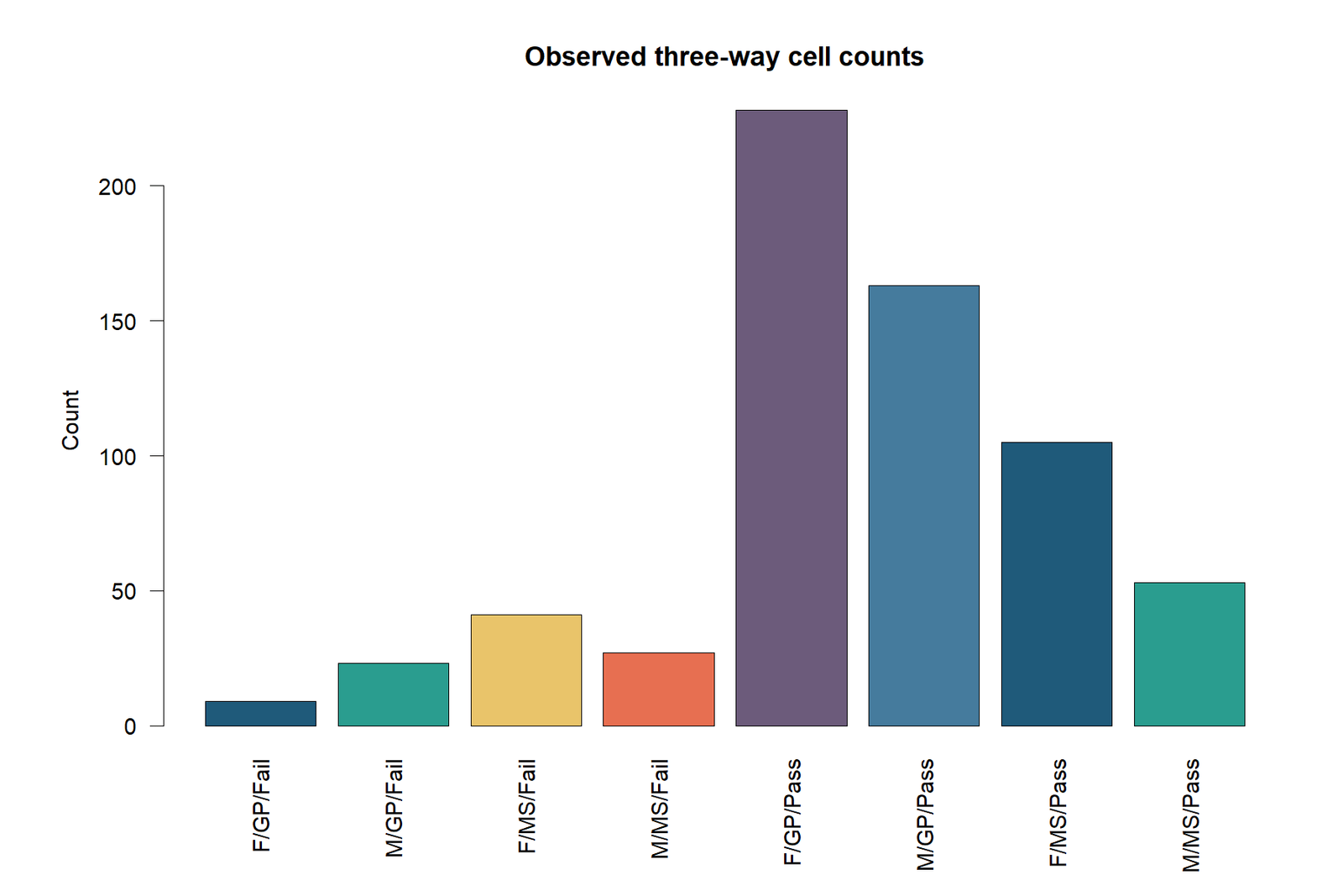
The 2 × 2 × 2 table contains eight cells: female and male students, GP and MS schools, and Pass or Fail status.
Model Structure
The fitted model includes school × sex, school × pass and sex × pass interactions. It omits only the school × sex × pass interaction.
Substantive Direction
Female students have higher pass rates in both schools, but the female–male difference is larger at GP. The male-versus-female pass odds ratio is 0.280 at GP and 0.766 at MS.
Hierarchical Log-Linear Formula
The model deliberately excludes λSXPijk. A significant residual deviance means that all two-way relationships are not sufficient to reproduce the observed eight-cell table.
Quick Answer: Categorical Data Analysis in R Result
Inferential Decision
- Null: no school × sex × pass interaction.
- Alternative: the two-variable association changes across the third variable.
- Decision: reject the pairwise-only model at α = .05.
- Conclusion: a three-way interaction is needed.
Substantive Interpretation
- GP female pass rate: 96.20%.
- GP male pass rate: 87.63%.
- MS female pass rate: 71.92%.
- MS male pass rate: 66.25%.
- The sex–pass odds ratio is more unequal at GP.
Table of Contents
- What is categorical data analysis in R?
- R methods for categorical variables
- Preparing categorical data for analysis in R
- Variables and data dictionary
- Observed three-way contingency table
- Hierarchical log-linear model
- Hypotheses and interaction meaning
- Complete model results
- Observed and fitted counts
- Residual and deviance diagnostics
What Is Categorical Data Analysis in R?
Definition
Categorical data analysis in R is the descriptive and inferential analysis of variables whose values represent categories. R supports one-way frequencies, two-way contingency tables, exact tests, binary models, multinomial models, ordinal models, survey-weighted analysis and multiway log-linear models.
R is particularly useful because one script can prepare factors, create tables, fit statistical models, calculate diagnostics and generate figures from the same reproducible analysis.
Why a Three-Way Example Is Valuable
A two-way chi-square test asks whether two categorical variables are associated. A three-way analysis asks whether that association remains stable after a third categorical variable is introduced.
The worked school × sex × pass table demonstrates how categorical data analysis in R moves from simple counts to a formal interaction test.
Descriptive, Inferential and Model-Based Layers
Frequency tables, percentages, bar charts, mosaic plots and observed cell counts.
Chi-square, exact conditional tests and likelihood-ratio comparisons.
Poisson log-linear models, logistic models, multinomial models and ordinal models.
Expected counts, fitted counts, Pearson residuals, deviance residuals and cell influence.
Conditional odds ratios, pass probabilities, interaction contrasts and uncertainty intervals.
Model formula, test statistic, df, p-value, cells driving the result and substantive limitations.
Why R Factors Matter
R factor levels determine table order, reference categories and coefficient interpretation. The worked categorical data analysis in R fixes school as GP then MS, sex as F then M, and pass status as Fail then Pass.
Choosing a Categorical Data Analysis Method in R
Use table(), prop.table(), binomial intervals or a goodness-of-fit test.
Use xtabs(), Pearson chi-square, exact methods and effect-size measures.
Use hierarchical log-linear models or a regression model with interaction terms.
Use binary logistic regression when predictors and adjusted effects are central.
Use ordinal logistic regression when category order should affect the model.
Why a Log-Linear Model Is Appropriate Here
All three variables are categorical and the research question concerns the association structure of the complete table. No single variable has to be declared the outcome in a log-linear model. The Poisson mean of each cell is modelled through main effects and interactions.
When Logistic Regression Gives an Equivalent View
If pass status is explicitly treated as the response, a logistic model containing school, sex and a school × sex interaction tests the same practical effect modification. The log-linear approach remains useful because it treats the three-way table symmetrically.
When Not to Use the Worked Model
The model is not appropriate for repeated observations, longitudinal responses, survey weights, multilevel clusters or continuous predictors without modification. Those settings require specialized categorical data analysis in R methods.
Preparing Categorical Data for Analysis in R
Clean the Original Fields
Inspect spelling, leading spaces, capitalization, missing values and unexpected codes. Convert empty strings to NA and print all levels before constructing the table.
Create the Binary Pass Variable
The worked R analysis defines Pass when G3 ≥ 10 and Fail when G3 < 10. The threshold must be stated because changing it creates a different contingency table and research question.
Recommended R Preparation Code
df <- read.csv("dataset.csv", stringsAsFactors = FALSE)

df$school <- factor(
  trimws(df$school),
  levels = c("GP", "MS")
)

df$sex <- factor(
  trimws(df$sex),
  levels = c("F", "M")
)

df$pass_status <- factor(
  ifelse(df$G3 >= 10, "Pass", "Fail"),
  levels = c("Fail", "Pass")
)

analysis <- df[
  complete.cases(df[, c("school", "sex", "pass_status")]),
]
Verify the Levels Before Fitting
levels(analysis$school)
levels(analysis$sex)
levels(analysis$pass_status)

table(analysis$school)
table(analysis$sex)
table(analysis$pass_status)
Why Category Preparation Changes Interpretation
R uses reference levels when producing model coefficients. Reversing F and M or Fail and Pass changes coefficient signs and odds-ratio direction. The fitted cell counts and global interaction test remain equivalent when the recoding is internally consistent.
See Variables in Statistics, Frequency Distribution and Cross-Tabulation for additional preparation and table-reading guidance.
Variables and Data Dictionary for Categorical Data Analysis in R
| Variable | Model role | Type | Coding | Valid N | Interpretation |
|---|---|---|---|---|---|
| school | Categorical factor | Nominal | GP, MS | 649 | School membership. |
| sex | Categorical factor | Binary nominal | F, M | 649 | Dataset variable for female and male students. |
| G3 | Source variable | Quantitative | Final grade | 649 | Used to derive pass status. |
| pass_status | Categorical factor | Binary | Fail when G3 < 10; Pass when G3 ≥ 10 | 649 | Final binary outcome category. |
| Freq | Poisson response | Count | Observed cell frequency | 8 cells | Response used by the log-linear model. |
GP Students
423 records.
MS Students
226 records.
Female Students
383 records.
Male Students
266 records.
Overall Pass and Fail Totals
The table contains 549 passes and 100 failures. Female students contribute 333 passes and 50 failures; male students contribute 216 passes and 50 failures. These margins do not reveal the significant three-way pattern until school is included.
Observed Three-Way Contingency Table
| Cell | Sex | School | Status | Observed count | Percent of all records |
|---|---|---|---|---|---|
| F/GP/Fail | F | GP | Fail | 9 | 1.39% |
| M/GP/Fail | M | GP | Fail | 23 | 3.54% |
| F/MS/Fail | F | MS | Fail | 41 | 6.32% |
| M/MS/Fail | M | MS | Fail | 27 | 4.16% |
| F/GP/Pass | F | GP | Pass | 228 | 35.13% |
| M/GP/Pass | M | GP | Pass | 163 | 25.12% |
| F/MS/Pass | F | MS | Pass | 105 | 16.18% |
| M/MS/Pass | M | MS | Pass | 53 | 8.17% |
| Total | — | — | — | 649 | 100.00% |
Failure Pattern
GP has 32 failures: 9 female and 23 male. MS has 68 failures: 41 female and 27 male. Failure counts must be interpreted with the sex-specific denominators in each school.
Pass Pattern
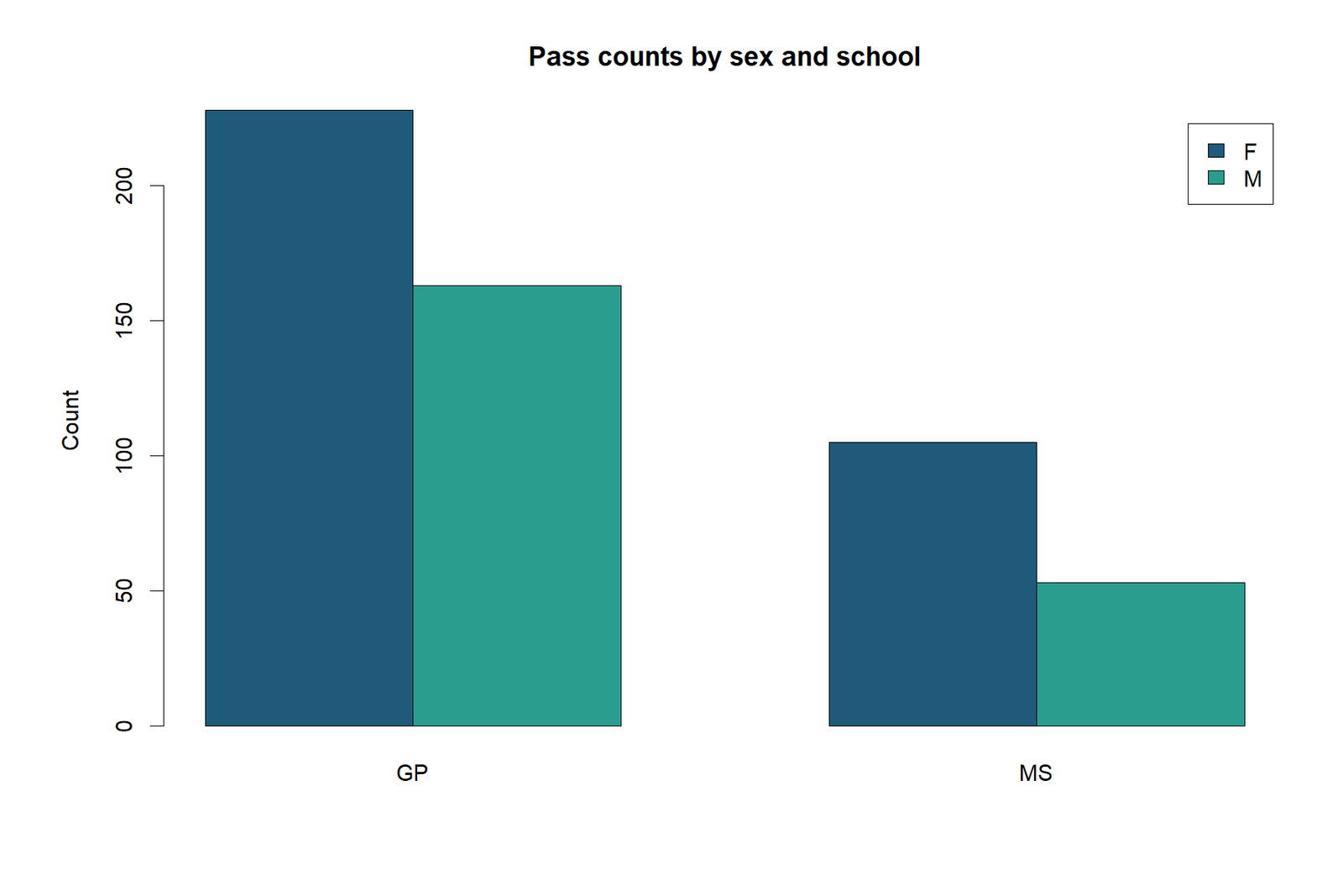
GP has 391 passes: 228 female and 163 male. MS has 158 passes: 105 female and 53 male. The pass-profile figure displays these four counts.
Why Eight Cells Are Needed
Collapsing over school would hide the fact that the sex–pass relationship changes between GP and MS. Collapsing over sex would similarly hide conditional pass differences. Multiway categorical data analysis in R preserves all eight combinations.
Hierarchical Log-Linear Model in R
Pairwise-Interaction Model
The fitted model contains all three main effects and all three two-way interactions:
In R formula syntax, this is Freq ~ (school + sex + pass_status)^2.
Saturated Comparison Model
The saturated model adds the three-way interaction:
With eight cells, the saturated model reproduces all observed counts exactly and has zero residual degrees of freedom.
Likelihood-Ratio Comparison
The residual deviance of the pairwise-interaction model equals its likelihood-ratio difference from the saturated model. A significant result indicates that the omitted three-way interaction explains remaining structure.
Worked Model Fit
Residual df = 1
Likelihood-ratio p = 0.040982
Pearson X² = 4.066339
Pearson p = 0.043746
AIC = 64.412
Meaning of Hierarchy
A hierarchical model containing the three-way interaction must also contain every lower-order main effect and two-way interaction. The pairwise-only model is also hierarchical because each included interaction retains its component main effects.
Hypotheses and Three-Way Interaction Meaning
Null Hypothesis
The school × sex, school × pass and sex × pass relationships fully explain the table. The sex–pass odds ratio is constant across schools.
Alternative Hypothesis
The association between two variables changes across the third. At least one conditional odds ratio differs.
Conditional Odds-Ratio Interpretation
| School | Female pass/fail | Male pass/fail | Male-vs-female pass OR | 95% CI |
|---|---|---|---|---|
| GP | 228/9 | 163/23 | 0.279748 | [0.126150, 0.620368] |
| MS | 105/41 | 53/27 | 0.766490 | [0.425989, 1.379161] |
The male-versus-female pass odds ratio is 0.280 at GP and 0.766 at MS. The MS-to-GP ratio of those odds ratios is 2.740, corresponding to a log interaction contrast of 1.008.
Direction of the Interaction
Female students have higher pass rates at both schools. The female advantage is stronger at GP because the male-versus-female odds ratio is farther below 1. The significant three-way test shows that the two sex-specific pass patterns cannot be summarized by one school-invariant sex–pass association.
Complete Categorical Data Analysis in R Results
| Model test | Statistic | df | P-value | Decision |
|---|---|---|---|---|
| Likelihood-ratio deviance | 4.176749826 | 1 | 0.040982223 | Reject no-three-way interaction. |
| Pearson goodness of fit | 4.066339335 | 1 | 0.043745981 | Confirms inadequate pairwise-only fit. |
Likelihood-Ratio Evidence
G²(1) = 4.177, p = 0.041. The pairwise-interaction model leaves statistically significant structure.
Pearson Confirmation
X²(1) = 4.066, p = 0.044. The alternative goodness-of-fit statistic supports the same decision.
Practical Meaning
The school-specific female–male pass differences are not proportional. The conditional association changes rather than remaining fixed.
Why a p-Value Near .04 Requires Careful Reporting
The result is just below .05, not overwhelmingly small. The appropriate interpretation reports the exact statistic, table counts and model diagnostics rather than describing the result as “highly significant.” A small change in coding, threshold or sampling could affect the boundary decision.
What the Result Does Not Establish
The model does not prove a causal school effect, a biological sex mechanism or an intervention effect. It identifies a conditional association pattern in the observed dataset.
Observed and Fitted Cell Counts
| Cell | Observed | Fitted without three-way interaction | Observed − fitted | Absolute difference |
|---|---|---|---|---|
| F/GP/Fail | 9 | 13.221167 | -4.221167 | 4.221167 |
| M/GP/Fail | 23 | 18.778833 | +4.221167 | 4.221167 |
| F/MS/Fail | 41 | 36.778833 | +4.221167 | 4.221167 |
| M/MS/Fail | 27 | 31.221167 | -4.221167 | 4.221167 |
| F/GP/Pass | 228 | 223.778833 | +4.221167 | 4.221167 |
| M/GP/Pass | 163 | 167.221167 | -4.221167 | 4.221167 |
| F/MS/Pass | 105 | 109.221167 | -4.221167 | 4.221167 |
| M/MS/Pass | 53 | 48.778833 | +4.221167 | 4.221167 |
Balanced Deviation Pattern
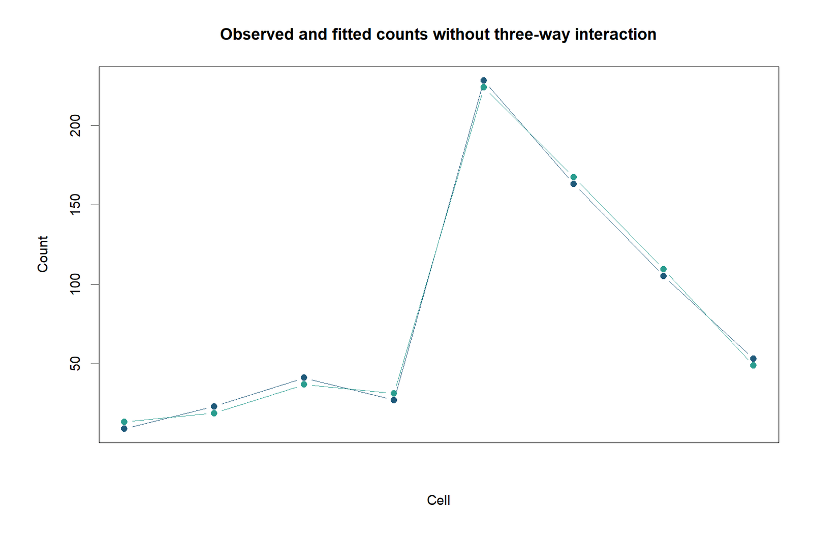
Every observed count differs from its fitted count by approximately 4.221 in absolute value. The signs alternate across the eight cells because the model preserves all two-way margins while omitting the single remaining three-way degree of freedom.
Cells Below the Fitted Count
F/GP/Fail, M/MS/Fail, M/GP/Pass and F/MS/Pass are below their pairwise-model fitted counts.
Cells Above the Fitted Count
M/GP/Fail, F/MS/Fail, F/GP/Pass and M/MS/Pass are above their pairwise-model fitted counts.
Why Fitted Counts Matter
Observed-versus-fitted comparisons show the direction of model failure. They also prevent the three-way interaction from being treated as an abstract p-value without a visible cell pattern.
Pearson Residuals and Deviance Components
| Cell | Pearson residual | Deviance component | Share of total deviance | Direction |
|---|---|---|---|---|
| F/GP/Fail | -1.160907 | 1.519632 | 36.38% | Below fitted |
| M/GP/Fail | +0.974088 | 0.884805 | 21.18% | Above fitted |
| F/MS/Fail | +0.696039 | 0.466931 | 11.18% | Above fitted |
| M/MS/Fail | -0.755454 | 0.598325 | 14.33% | Below fitted |
| F/GP/Pass | +0.282178 | 0.079128 | 1.89% | Above fitted |
| M/GP/Pass | -0.326428 | 0.107463 | 2.57% | Below fitted |
| F/MS/Pass | -0.403905 | 0.165282 | 3.96% | Below fitted |
| M/MS/Pass | +0.604389 | 0.355183 | 8.50% | Above fitted |
Largest Cell Contribution
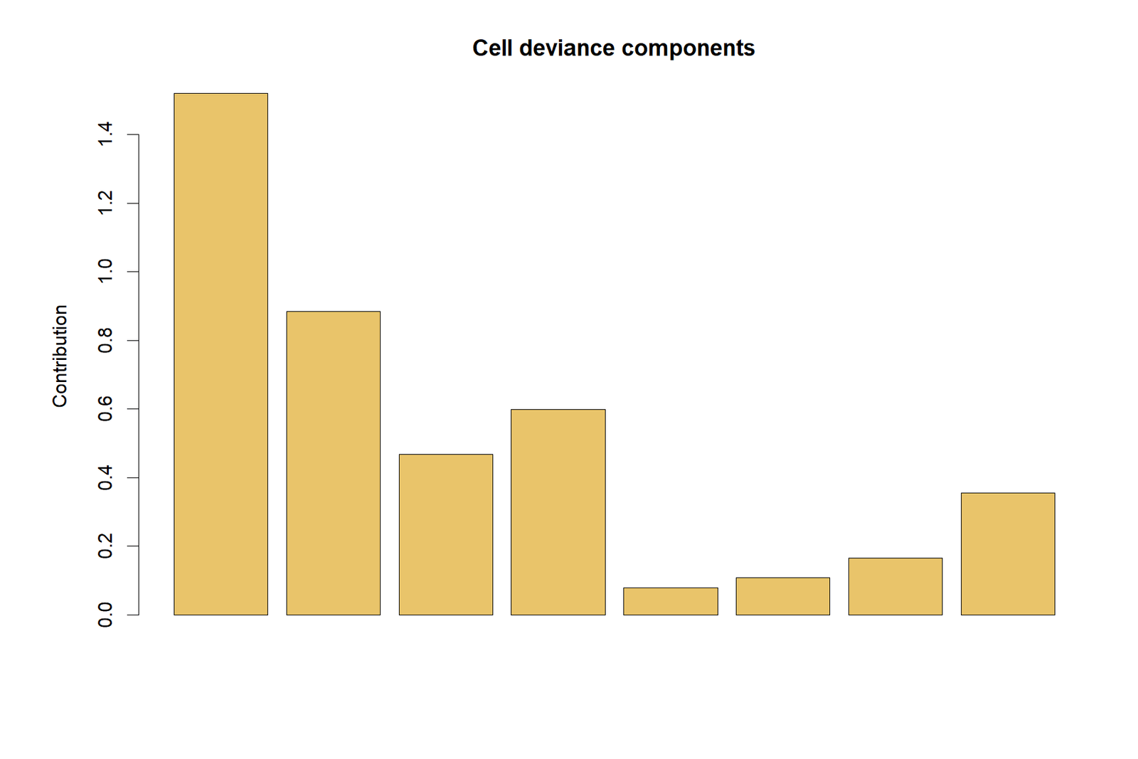
F/GP/Fail contributes 1.520, or 36.38% of total deviance. Its observed count of 9 is below the fitted count of 13.22.
Residual Magnitudes
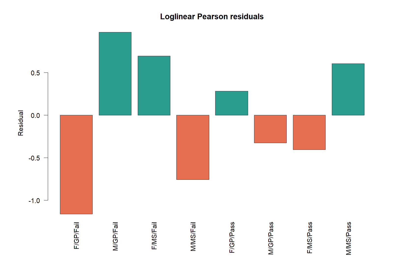
The largest absolute Pearson residual is 1.161. No single residual exceeds 2, but the structured eight-cell pattern produces a significant one-degree-of-freedom test.
Why Small Residuals Can Produce a Significant Interaction
The omitted three-way interaction has only one degree of freedom. All eight deviations represent the same structured contrast under fixed lower-order margins. The test aggregates that coordinated pattern rather than treating each cell as an unrelated discrepancy.
Deviance Contribution Formula
The eight cell components sum to the model deviance of 4.176750. Cell contributions identify where the model fails but should not be interpreted as eight independent hypothesis tests.
Pass Profiles by School and Student Sex
| School | Sex | Pass | Fail | Total | Pass rate |
|---|---|---|---|---|---|
| GP | F | 228 | 9 | 237 | 96.20% |
| GP | M | 163 | 23 | 186 | 87.63% |
| MS | F | 105 | 41 | 146 | 71.92% |
| MS | M | 53 | 27 | 80 | 66.25% |
GP Profile
Female students pass at 96.20% and male students at 87.63%. The difference is 8.57 percentage points.
MS Profile
Female students pass at 71.92% and male students at 66.25%. The difference is 5.67 percentage points.
Counts Versus Rates
The pass-profile figure displays pass counts, which are useful for showing the data volume. Statistical interpretation also needs the within-sex denominators because GP and MS have different sample sizes.
Conditional Effect Interpretation
The female advantage appears in both schools, but it is larger on the odds scale at GP. This changing conditional association is the substantive form of the significant three-way interaction.
R Analysis Procedure
1. Prepare Factors
Clean labels, set factor levels and derive pass status.
2. Build the Three-Way Table
Use xtabs() or table() and verify all eight cells.
3. Convert to Cell Data
Use as.data.frame() so each row contains factor levels and a frequency.
4. Fit the Pairwise Model
Use a Poisson GLM with every two-way interaction.
5. Compare With Saturated Fit
Test whether adding the three-way interaction improves fit.
6. Diagnose and Report
Extract fitted counts, residuals, deviance components and conditional profiles.
Recommended Base-R Functions
factor()
ifelse()
xtabs()
as.data.frame()
glm()
anova()
fitted()
residuals()
pchisq()
Why Base R Is Sufficient
This categorical data analysis in R can be reproduced with
base and recommended R functions. External packages may extend presentation,
exact testing or survey support, but they are not required for the hierarchical
Poisson model used here.
Reproducibility and Result Verification
Reproducibility is strengthened by retaining the observed table, fitted-count table, model summary, likelihood-ratio comparison, residual diagnostics and pass profiles with the analysis script. These results make every reported statistic traceable to the underlying cell counts.
Visual Results and Model Findings
The six R figures are organized into three result groups. Each figure is followed by its statistical meaning, exact values and interpretive takeaway.
Observed Three-Way Frequency Structure
Pattern: Pass cells are much larger than fail cells. F/GP/Pass is the largest cell, while F/GP/Fail is the smallest.
Statistical meaning: The plot verifies the complete 2 × 2 × 2 table before the log-linear model is fitted. It also shows why percentages and conditional effects are needed beside raw counts.
Interpretive takeaway: State all eight counts or provide the complete three-way table.
Where the Pairwise Model Misses the Data
Pattern: Observed and fitted series are close but consistently separated by about 4.22 counts in alternating directions.
Statistical meaning: The coordinated deviations form the single omitted three-way contrast. The global test determines whether that contrast is larger than expected by sampling variation.
Interpretive takeaway: Explain model failure through observed-versus-fitted cells, not only the p-value.
Direction of the Remaining Interaction Pattern
Pattern: Four residuals are positive and four are negative. F/GP/Fail has the largest negative residual, and M/GP/Fail has the largest positive residual.
Statistical meaning: The residual signs identify cells above or below the fitted pairwise model. Their alternating pattern is characteristic of the remaining three-way contrast.
Interpretive takeaway: Use residuals to explain direction, while the global one-df test controls the formal decision.
Cells Contributing Most to Model Deviance
Pattern: F/GP/Fail supplies the largest contribution, followed by M/GP/Fail and M/MS/Fail.
Statistical meaning: The failure cells are especially informative for the three-way interaction because their conditional proportions differ sharply across school and sex.
Interpretive takeaway: Identify influential cells without converting each component into a separate significance test.
Conditional Pass Profiles by School
Pattern: Female pass counts exceed male pass counts in both schools, but the count plot reflects unequal sex and school sample sizes.
Statistical meaning: Within-group pass rates and conditional odds ratios show that the female–male pass association is stronger at GP than at MS.
Interpretive takeaway: Pair pass counts with pass rates of 96.20%, 87.63%, 71.92% and 66.25%.
Final Interaction-Test Decision
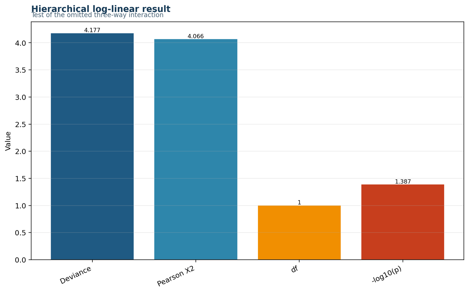
Pattern: The likelihood-ratio and Pearson statistics are both just above 4 with one degree of freedom. The negative log10 p-value is approximately 1.387.
Statistical meaning: Both goodness-of-fit measures reject the pairwise-only model at the .05 level and support including the three-way interaction.
Interpretive takeaway: Report the exact p-value as .041 rather than describing it only as significant.
Expandable Categorical Data Analysis in R Code
Prepare factors and build the three-way table
df <- read.csv(
  "dataset.csv",
  stringsAsFactors = FALSE
)

df$school <- factor(
  df$school,
  levels = c("GP", "MS")
)

df$sex <- factor(
  df$sex,
  levels = c("F", "M")
)

df$pass_status <- factor(
  ifelse(df$G3 >= 10, "Pass", "Fail"),
  levels = c("Fail", "Pass")
)

three_way_table <- xtabs(
  ~ sex + school + pass_status,
  data = df
)

print(three_way_table)
Convert the table to cell-frequency data
cells <- as.data.frame(
  three_way_table
)

names(cells)[
  names(cells) == "Freq"
] <- "Freq"

cells <- cells[
  order(
    cells$pass_status,
    cells$school,
    cells$sex
  ),
]

print(cells)
Fit the model without the three-way interaction
pairwise_model <- glm(
  Freq ~ (
    sex + school + pass_status
  )^2,
  family = poisson(link = "log"),
  data = cells
)

summary(pairwise_model)

deviance_value <- deviance(
  pairwise_model
)

df_value <- df.residual(
  pairwise_model
)

deviance_p <- pchisq(
  deviance_value,
  df = df_value,
  lower.tail = FALSE
)
Fit and compare the saturated model
saturated_model <- glm(
  Freq ~ sex * school * pass_status,
  family = poisson(link = "log"),
  data = cells
)

anova(
  pairwise_model,
  saturated_model,
  test = "Chisq"
)
The deviance difference is the test of the omitted school × sex × pass interaction.
Calculate Pearson goodness of fit
pearson_residuals <- residuals(
  pairwise_model,
  type = "pearson"
)

pearson_x2 <- sum(
  pearson_residuals^2
)

pearson_p <- pchisq(
  pearson_x2,
  df = df.residual(pairwise_model),
  lower.tail = FALSE
)

c(
  Pearson_X2 = pearson_x2,
  df = df.residual(pairwise_model),
  p_value = pearson_p
)
Extract fitted counts and deviance components
diagnostics <- transform(
  cells,
  Fitted = fitted(pairwise_model),
  PearsonResidual = residuals(
    pairwise_model,
    type = "pearson"
  ),
  DevianceComponent = residuals(
    pairwise_model,
    type = "deviance"
  )^2
)

diagnostics$Difference <-
  diagnostics$Freq - diagnostics$Fitted

print(diagnostics)
Calculate pass rates by school and sex
pass_table <- xtabs(
  ~ school + sex + pass_status,
  data = df
)

pass_rates <- prop.table(
  pass_table,
  margin = c(1, 2)
)

round(
  100 * pass_rates[, , "Pass"],
  2
)
Calculate conditional male-versus-female odds ratios
gp <- matrix(
  c(163, 23, 228, 9),
  nrow = 2,
  byrow = TRUE,
  dimnames = list(
    Sex = c("M", "F"),
    Status = c("Pass", "Fail")
  )
)

ms <- matrix(
  c(53, 27, 105, 41),
  nrow = 2,
  byrow = TRUE,
  dimnames = list(
    Sex = c("M", "F"),
    Status = c("Pass", "Fail")
  )
)

or_gp <- (
  gp["M", "Pass"] * gp["F", "Fail"]
) / (
  gp["M", "Fail"] * gp["F", "Pass"]
)

or_ms <- (
  ms["M", "Pass"] * ms["F", "Fail"]
) / (
  ms["M", "Fail"] * ms["F", "Pass"]
)

c(GP = or_gp, MS = or_ms)
Create the observed-cell bar figure
cell_labels <- with(
  cells,
  paste(sex, school, pass_status, sep = "/")
)

barplot(
  height = cells$Freq,
  names.arg = cell_labels,
  las = 2,
  ylab = "Count",
  main = "Observed three-way cell counts"
)
Create observed-versus-fitted and residual figures
plot(
  diagnostics$Freq,
  type = "b",
  pch = 19,
  xlab = "Cell",
  ylab = "Count",
  main = "Observed and fitted counts"
)

lines(
  diagnostics$Fitted,
  type = "b",
  pch = 19
)

barplot(
  diagnostics$PearsonResidual,
  names.arg = cell_labels,
  las = 2,
  ylab = "Residual",
  main = "Loglinear Pearson residuals"
)
Assumptions, Diagnostics and Limitations
Independent Records
Each student should contribute to one and only one three-way cell.
Correct Category Coding
School, sex and pass levels must be mutually exclusive and consistently defined.
Adequate Cell Information
Very sparse cells can make asymptotic model comparisons unstable.
Poisson sampling assumption
Log-linear models treat cell counts as Poisson variables. Under multinomial or product-multinomial sampling, the same likelihood-ratio tests remain closely connected when the correct margins and model structure are used.
Independence of observations
The model assumes independent student records. School or classroom clustering can require a multilevel or marginal model instead of a simple eight-cell table.
Hierarchical model principle
Higher-order interactions should not be included while their component lower-order terms are deleted. The worked models respect hierarchy.
Sparse-cell assessment
The smallest observed count is 9, so no cell is zero. Nevertheless, failure cells are much smaller than pass cells and deserve careful diagnostic inspection.
Pass-threshold sensitivity
Defining Pass as G3 ≥ 10 is a substantive coding decision. Another threshold would produce different counts and potentially a different interaction result.
Borderline p-value
The likelihood-ratio p-value is .041. The result should be described accurately and not exaggerated as overwhelming evidence.
Causal interpretation
The interaction is associational. It does not show that school or sex causes passing.
Original quantitative information
Dichotomizing G3 discards grade distance. A complementary model of the original grade can preserve more information.
Alternative effect scales
A three-way log-linear interaction describes changing odds associations. Risk differences or probability contrasts may show a different practical pattern.
Multiple exploratory tables
Testing many thresholds and variable combinations increases false-positive risk. Primary models should be prespecified.
Advanced Categorical Data Analysis in R Topics
Exploratory Analysis of Categorical Data in R
Within categorical data analysis in R, exploratory analysis begins with frequency tables, missing-value patterns, category ordering, two-way percentages and graphical summaries. Exploratory data analysis of categorical variables in R should identify sparse levels and unexpected labels before inferential testing.
Univariate Analysis of Categorical Data in R
Within categorical data analysis in R, a single factor can be summarized with counts, proportions, confidence intervals and goodness-of-fit tests. The denominator and missing-data rule should always be visible.
Analysis of Ordinal Categorical Data in R
Within categorical data analysis in R, ordinal categories contain rank information. Trend tests, cumulative-link models and proportional-odds models can use that order more efficiently than a nominal chi-square or log-linear model.
Categorical Survey Data Analysis in R
Within categorical data analysis in R, survey weights, strata and clusters require design-based estimators and adjusted tests. An ordinary unweighted table is not a substitute for survey-aware categorical analysis.
Longitudinal Categorical Data Analysis in R
Within categorical data analysis in R, repeated categorical outcomes require methods such as generalized estimating equations, transition models or mixed-effects logistic models. Ordinary log-linear independence assumptions do not handle within-person repetition.
Cluster Analysis on Categorical Data in R
Within categorical data analysis in R, clustering categorical observations requires a suitable dissimilarity or model-based approach. Euclidean distance on arbitrary category codes is generally inappropriate.
Tree Analysis in R With Categorical Data
Within categorical data analysis in R, classification trees can predict a categorical outcome and discover interactions, but cross-validation and pruning are needed to control overfitting.
Log-Linear Versus Logistic Models
Within categorical data analysis in R, a log-linear model treats the full table symmetrically. Logistic regression designates an outcome and produces adjusted odds ratios. Equivalent interaction questions can often be expressed in both frameworks.
Structural Zeros
Within categorical data analysis in R, a structural zero represents an impossible cell and changes the sample space. It should not be treated as an ordinary observed zero or repaired with an arbitrary constant.
Model Selection With More Variables
Within categorical data analysis in R, four-way and higher tables contain many possible interactions. Scientific hierarchy, likelihood-ratio comparisons and parsimonious model selection are essential.
Exact and Monte Carlo Alternatives
Within categorical data analysis in R, when tables are sparse, exact conditional or Monte Carlo procedures can reduce reliance on asymptotic chi-square references.
Categorical Data Analysis in R With a Categorical Predictor
Within categorical data analysis in R, when one factor is clearly a predictor and another is an outcome, logistic, multinomial or ordinal regression provides coefficient-based interpretation and predicted probabilities.
Preparing Categorical Data for Analysis in R
Within categorical data analysis in R, good preparation includes factor-level validation, missing-data checks, reference-category selection, sparse-level review and reproducible derived-variable definitions.
Complete Categorical Analysis Sequence
Within categorical data analysis in R, a complete analysis
moves from observed counts to percentages, model specification, model
comparison, residual diagnostics, conditional effects and an APA-ready result.
APA Reporting for Categorical Data Analysis in R
An APA-style log-linear report should identify the three variables, table dimensions, model hierarchy, omitted interaction, likelihood-ratio statistic, degrees of freedom, p-value, Pearson confirmation and the conditional pattern that explains the interaction.
Full Worked APA Result
A hierarchical log-linear analysis examined the association among school, student sex and pass status (G3 ≥ 10), N = 649. A model containing all main effects and two-way interactions but excluding the school × sex × pass interaction did not fit the observed 2 × 2 × 2 table adequately, likelihood-ratio G²(1) = 4.18, p = 0.041, Pearson X²(1) = 4.07, p = 0.044. The male-versus-female pass odds ratio was 0.28 at GP and 0.77 at MS, indicating that the sex–pass association differed by school.
Concise APA Result
The no-three-way-interaction log-linear model was rejected, G²(1) = 4.18, p = 0.041. The association between student sex and pass status varied across GP and MS.
APA-Style Methods Sentence
School, sex and pass status were cross-classified in a 2 × 2 × 2 table, and a Poisson hierarchical log-linear model containing every two-way interaction was compared with the saturated model to test the omitted three-way interaction.
APA Results Table
| Measure | Complete value | APA presentation |
|---|---|---|
| Sample size | 649 | N = 649 |
| Table dimensions | 2 × 2 × 2 | 2 × 2 × 2 table |
| Likelihood-ratio deviance | 4.176749826 | G² = 4.18 |
| Degrees of freedom | 1 | df = 1 |
| Likelihood-ratio p-value | 0.040982223 | p = 0.041 |
| Pearson statistic | 4.066339335 | X² = 4.07 |
| Pearson p-value | 0.043745981 | p = 0.044 |
| GP male/female pass OR | 0.279748284 | OR = 0.28 |
| MS male/female pass OR | 0.766490300 | OR = 0.77 |
Reusable APA Templates
Significant Three-Way Interaction
A hierarchical log-linear model analysed factor A, factor B and factor C, N = N.
The model without the three-way interaction was rejected, G²(df) = statistic, p = p-value.
The association between two variables differed across the third variable.
Describe conditional counts, rates or odds ratios after the global interaction result.
No Detected Three-Way Interaction
A model containing all two-way interactions was fitted to a dimensions table.
The residual deviance was not significant, G²(df) = statistic, p = p-value.
The data did not provide sufficient evidence that the two-variable association varied across the third factor.
Nonsignificance does not prove that the conditional associations are identical.
Model-Fit and Residual Follow-Up
Pearson X²(df) = statistic, p = p-value.
The largest model departure occurred in cell, Pearson residual = residual.
Conditional odds ratios were OR 1 and OR 2 across the two strata.
Residuals explain the model test; they do not replace it.
APA Language Rules
| Avoid | Use instead | Reason |
|---|---|---|
| The variables were correlated. | The categorical association differed by school. | Correlation is not the general term for a log-linear interaction. |
| The p-value was highly significant. | G²(1) = 4.18, p = .041. | The exact borderline value should remain visible. |
| School caused the sex difference. | The sex–pass association varied across schools. | The observational table does not establish causality. |
| Every residual was significant. | Describe the global interaction and the residual pattern. | Residual bars are diagnostic, not independent tests. |
Common Mistakes and Final Reporting Checklist
Common Mistakes
| Mistake | Correction |
|---|---|
| Fitting the model before checking factor levels | Print and order every category first. |
| Calling the three-way interaction a main effect | Explain that a two-variable association changes across the third variable. |
| Deleting lower-order terms from a hierarchical model | Retain all component main effects and two-way interactions. |
| Reporting only the deviance p-value | Add observed counts, fitted counts, residuals and conditional profiles. |
| Using raw pass counts as rates | Report within-school and within-sex denominators. |
| Interpreting p = .041 as overwhelming | Report the exact value and acknowledge boundary sensitivity. |
| Calling sex “gender” when the dataset variable is sex | Use the original variable name and female/male labels accurately. |
| Claiming causation from the table | Use conditional association language. |
Statistical Reporting Checklist
- Define all three categorical variables and their levels.
- State the pass threshold and valid sample size.
- Show the complete eight-cell table.
- Write the hierarchical model formula.
- Name the omitted three-way interaction.
- Report G², df and the exact p-value.
- Report Pearson X² as a model-fit confirmation.
- Show observed and fitted counts.
- Interpret residual direction and deviance contributions.
- Report school-specific pass rates and odds ratios.
- Present the observed-count, fitted-count, residual, deviance, pass-profile and result-summary figures.
- State the observational limitations and avoid causal language.
Categorical Data Analysis in R Figure Downloads
Observed and Fitted CountsDownload the pairwise-model fit comparison.
Pearson ResidualsDownload the signed log-linear residual figure.
Deviance ComponentsDownload cell-level likelihood-ratio contributions.
Pass ProfilesDownload pass counts by school and student sex.
Model Result SummaryDownload the G², Pearson, df and p-value summary.
Frequently Asked Questions About Categorical Data Analysis in R
What is categorical data analysis in R?
Within categorical data analysis in R, it is the use of R to summarize, test and model variables represented by categories.
What is the worked R example?
Within categorical data analysis in R, a three-way school × sex × pass-status table with 649 student records.
What is a log-linear model?
Within categorical data analysis in R, it is a Poisson model for contingency-table cell counts using categorical main effects and interactions.
What model is fitted here?
Within categorical data analysis in R, all main effects and all two-way interactions are included; the three-way interaction is initially omitted.
What is the null hypothesis?
Within categorical data analysis in R, the school × sex × pass interaction is zero and the two-variable associations do not change across the third factor.
What is the likelihood-ratio statistic?
Within categorical data analysis in R, g² = 4.176750.
What are the degrees of freedom?
Within categorical data analysis in R, there is one residual degree of freedom.
What is the p-value?
Within categorical data analysis in R, the likelihood-ratio p-value is 0.040982, reported as .041.
What is the Pearson result?
Within categorical data analysis in R, pearson X² = 4.066339, p = 0.043746.
What is the conclusion?
Within categorical data analysis in R, the model without the three-way interaction is rejected.
What does the interaction mean?
Within categorical data analysis in R, the association between student sex and pass status differs across GP and MS.
What are the GP pass rates?
Within categorical data analysis in R, female GP students pass at 96.20% and male GP students at 87.63%.
What are the MS pass rates?
Within categorical data analysis in R, female MS students pass at 71.92% and male MS students at 66.25%.
What is the GP male-versus-female pass odds ratio?
Within categorical data analysis in R, it is 0.279748.
What is the MS male-versus-female pass odds ratio?
Within categorical data analysis in R, it is 0.766490.
Which cell contributes most to deviance?
Within categorical data analysis in R, f/GP/Fail contributes 1.520.
Are any observed cells zero?
Within categorical data analysis in R, no. The smallest observed cell count is 9.
Why are fitted counts useful?
Within categorical data analysis in R, they show the cell pattern that the pairwise-only model cannot reproduce.
Why can residuals below 2 still produce significance?
The one-degree-of-freedom test aggregates a coordinated eight-cell interaction contrast.
How do I create the table in R?
Use xtabs(~ sex + school + pass_status, data=df).
How do I fit the model in R?
Use glm(Freq ~ (sex + school + pass_status)^2, family=poisson, data=cells).
How do I test the three-way interaction?
Compare the pairwise model with the saturated model using a likelihood-ratio chi-square test.
Is categorical data analysis in R limited to chi-square tests?
No. R supports log-linear, logistic, multinomial, ordinal, survey and longitudinal methods.
How is ordinal categorical data analysed in R?
Use ordered factors and an ordinal model or trend test when the order is substantively important.
How is categorical survey data analysed in R?
Use survey weights, strata and clusters through a design-aware analysis.
How is longitudinal categorical data analysed in R?
Use repeated-response methods such as GEE, transition models or mixed-effects logistic models.
Can R perform exploratory analysis of categorical variables?
Yes. Frequencies, percentages, mosaic displays and cross-tabulations are standard exploratory tools.
Can a tree use categorical data in R?
Yes, but the model should be validated and pruned to control overfitting.
What should APA reporting include?
The variables, model hierarchy, G², df, p-value, Pearson confirmation, conditional effects and limitations.
What is the main conclusion?
The sex–pass association changes across schools, so the three-way interaction is needed.
Categorical Data Analysis in R Conclusion
Statistical Conclusion
The hierarchical pairwise-interaction model produced G²(1) = 4.176750, p = 0.040982, and Pearson X²(1) = 4.066339, p = 0.043746. The model without the three-way interaction was rejected.
Substantive Conclusion
Female students had higher pass rates in both schools, but the conditional sex–pass association was stronger at GP. The male-versus-female pass odds ratio was 0.280 at GP and 0.766 at MS.
A complete categorical data analysis in R connects factor
preparation, observed tables, model hierarchy, fitted counts, residuals, deviance
components and conditional profiles with a clear statistical interpretation.
The six figures connect each diagnostic result to the underlying model findings.

