
Cochran’s Q Test: Formula, Interpretation, Post Hoc Comparisons, Python, R, SPSS and Excel Guide
Cochran’s Q Test is the standard extension of chi-square-style categorical inference from two matched binary responses to three or more matched binary responses. This complete guide explains the hypotheses, formula, assumptions, hand calculation, post hoc logic, Python, R, SPSS and Excel workflows, charts, APA reporting and downloadable reports by analysing four related yes/no responses for 649 students: school support, family support, paid classes and activities.
4 binary conditions
Q = 639.2472
df = 3, p ≈ 3.12 × 10−138
What Is Cochran’s Q Test?
Cochran’s Q Test is a nonparametric repeated-measures test for dichotomous data. It is used when the same participants are observed under three or more related conditions and each condition is recorded as 0/1, no/yes, fail/pass or absent/present. If you need a broader introduction to matched categorical analysis, see cross-tabulation, two-way tables and relative frequencies and categorical data analysis in Python.
Conceptually, Cochran’s Q Test asks whether the success probabilities are identical across all repeated binary conditions after accounting for the fact that the measurements come from the same subjects. It is therefore a natural extension of chi-square test of independence ideas to a matched-subject design, and a natural extension of McNemar-style reasoning from two related responses to many related responses.
What question does the worked example answer?
In the current dataset, the same 649 students each answered four binary items: schoolsup, famsup, paid and activities. The research question is whether the probability of a “yes” response is equal across these four related conditions. The four conditions represent different support or activity indicators, so treating them as independent samples would violate the matched design.
If you want help writing formal hypotheses, see null and alternative hypothesis, p-value and type I and type II error.
Quick Answer: Cochran’s Q Test Result
The repeated binary analysis is based on 649 matched students and four yes/no conditions. The verified workbook, Python, R and SPSS outputs all agree on the same result.
Test summary
- Procedure: Cochran’s Q Test for related dichotomous responses
- Conditions: school support, family support, paid classes, activities
- Statistic: Q = 639.2472
- Degrees of freedom: df = 3
- P-value: approximately 3.12 × 10−138
- Decision: reject the null of equal response probabilities
Practical meaning
- Family support is reported much more often than the other responses.
- Activities is also common, but less common than family support.
- School support and paid classes are both uncommon.
- The pattern difference is not only statistically significant; it is visibly large.
- Pairwise follow-up comparisons are justified after the global test.
Table of Contents
- When to use Cochran’s Q Test
- Formula and hand calculation
- Variables and data dictionary
- Observed results and interpretation
- Post hoc comparisons after Cochran’s Q
- Python charts
- R chart pairs
- Python, R, SPSS and Excel workflows
- Code and software notes
- Assumptions and common mistakes
- APA reporting
- Downloads
- Related guides
- Frequently asked questions
- Conclusion
When to Use Cochran’s Q Test
Use Cochran’s Q Test when
- The same participants are measured repeatedly or under multiple related conditions.
- Each outcome is binary: yes/no, pass/fail, present/absent or 1/0.
- There are three or more related conditions.
- You need a global test before exploring pairwise differences.
- The design is matched, blocked or repeated rather than independent.
Choose another method when
- The groups are independent instead of matched; then consider chi-square test of homogeneity.
- The table is a single two-variable cross-tab; then consider chi-square test of independence.
- The response has more than two categories.
- The outcome is quantitative; then t tests, ANOVA or other repeated-measures approaches may be more appropriate.
- You need covariate adjustment; then logistic regression or other repeated-model frameworks may be better.
If yes, stay in the matched-data family.
If yes, Cochran’s Q may be suitable.
If yes, Cochran’s Q is the standard global test.
Cochran’s Q Test Formula and Hand Calculation
The workbook and software use the standard Q statistic:
\[k\sum C_j^2 − T^2\] ÷ \[kT − \sum R_i^2\]
| Symbol | Meaning | Worked value |
|---|---|---|
| k | Number of related binary conditions | 4 |
| Cj | Column total of successes for condition j | 68, 398, 39, 315 |
| T | Total successes across all conditions | 820 |
| Ri | Row total of successes for subject i | 0 to 4 per student |
| ΣCj2 | Sum of squared column totals | 263,774 |
| ΣRi2 | Sum of squared row totals | 1,484 |
Step 1: Compute the column totals
Step 2: Square and sum the column totals
Step 3: Sum the squared subject totals
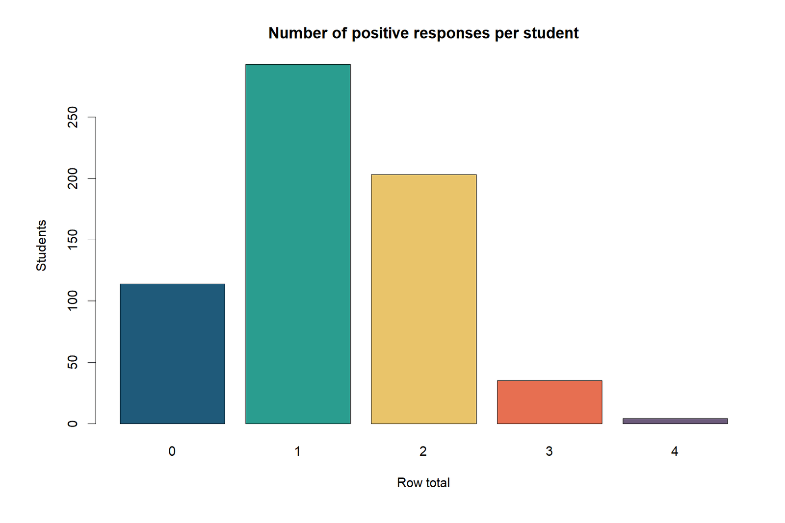
Each student contributes a row total from 0 through 4. Using the row-total distribution 114, 293, 203, 35 and 4 for totals 0, 1, 2, 3 and 4 respectively:
Step 4: Substitute into the Q formula
Step 5: Compare with a chi-square reference distribution
Under the null, Q is approximately chi-square distributed with 3 degrees of freedom. The resulting p-value is 3.1237986523292055 × 10−138, which is effectively zero to ordinary reporting precision.
Variables and Data Dictionary
schoolsup, famsup, paid and activities, coded yes = 1 and no = 0.| Variable | Meaning | Binary event | Yes count | Proportion |
|---|---|---|---|---|
| schoolsup | Extra educational support from school | yes = 1 | 68 | 0.1047766 |
| famsup | Family educational support | yes = 1 | 398 | 0.6132512 |
| paid | Paid extra classes | yes = 1 | 39 | 0.0600924 |
| activities | Extra-curricular activities | yes = 1 | 315 | 0.4853621 |
Row-total distribution
| Number of “yes” responses for a student | Count of students | Interpretation |
|---|---|---|
| 0 | 114 | No positive responses on any of the four conditions. |
| 1 | 293 | Exactly one condition marked yes. |
| 2 | 203 | Exactly two conditions marked yes. |
| 3 | 35 | Exactly three conditions marked yes. |
| 4 | 4 | All four conditions marked yes. |
This row-total pattern matters because Cochran’s Q is not based only on column percentages. The subject-level structure determines the denominator through ΣRi2. For related concepts, see frequency and relative frequency tables, descriptive statistics and effect size.
Observed Results and Interpretation
68 yes, 581 no
398 yes, 251 no
39 yes, 610 no
315 yes, 334 no
Global repeated-binary test
Extremely small
| Metric | Value | Interpretation |
|---|---|---|
| Number of conditions | 4 | Four related binary variables were compared. |
| Number of students | 649 | All repeated responses come from the same 649 rows. |
| Total successes | 820 | Total yes responses across all conditions. |
| Q statistic | 639.2472160 | Large departure from equal response probabilities. |
| Degrees of freedom | 3 | Equal to k − 1. |
| P-value | 3.1237986523292055e-138 | Reject the null hypothesis decisively. |
What the result means
The data provide overwhelming evidence that the four related yes-probabilities are not equal. Family support is reported far more often than school support or paid classes, and activities is also much more frequent than school support and paid classes. In other words, the within-student pattern is highly unbalanced across conditions.
Because the p-value is extremely small, the global decision is clear even if a stricter significance level is used. However, the global test alone does not say which pairs differ. That question belongs to post hoc comparisons, explained next. For reporting language, see p-value, significance level and test statistic and confidence interval.
Post Hoc Comparisons After Cochran’s Q Test
A significant Cochran’s Q Test should normally be followed by planned or multiplicity-adjusted pairwise comparisons. The common follow-up is McNemar testing for each pair, because each pair still consists of two related binary conditions measured on the same subjects. If you need multiple-comparison background, see Bonferroni correction, Holm-Bonferroni method and pairwise comparisons after ANOVA for general multiplicity ideas.
| Pair | b = first yes, second no | c = first no, second yes | Discordance pattern | Interpretation |
|---|---|---|---|---|
| schoolsup vs famsup | 19 | 349 | Far more famsup-only than schoolsup-only | Family support is much more common. |
| schoolsup vs paid | 62 | 33 | Moderate imbalance | School support is more common than paid classes. |
| schoolsup vs activities | 38 | 285 | Far more activities-only than schoolsup-only | Activities is much more common. |
| famsup vs paid | 367 | 8 | Extremely unbalanced | Family support is much more common. |
| famsup vs activities | 206 | 123 | Clear imbalance | Family support exceeds activities. |
| paid vs activities | 15 | 291 | Extremely unbalanced | Activities is much more common. |
Every pair above shows a strong discordance imbalance, so the follow-up story is consistent with the overall ordering of the four response proportions. The pairwise p-value chart visualizes the same idea. When teaching this in an AP Statistics setting, it is useful to emphasize that the global test answers “is anything different?” while pairwise tests answer “which specific pairs differ?”
Python Chart Interpretation
Chart 1: Condition successesPython
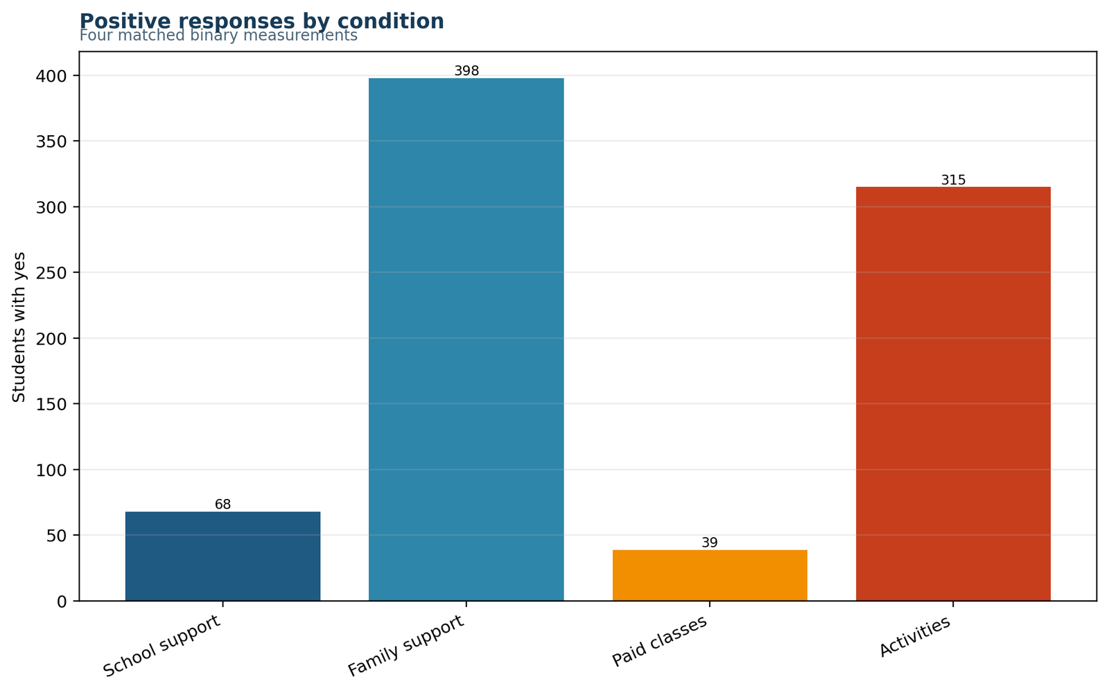
The four bars are highly uneven, with family support highest and paid classes lowest.
Counts are 68, 398, 39 and 315.
This visual already suggests that the equal-probability null is implausible.
The Q statistic is driven largely by these unequal column totals after matching is accounted for.
Chart 2: Condition proportionsPython
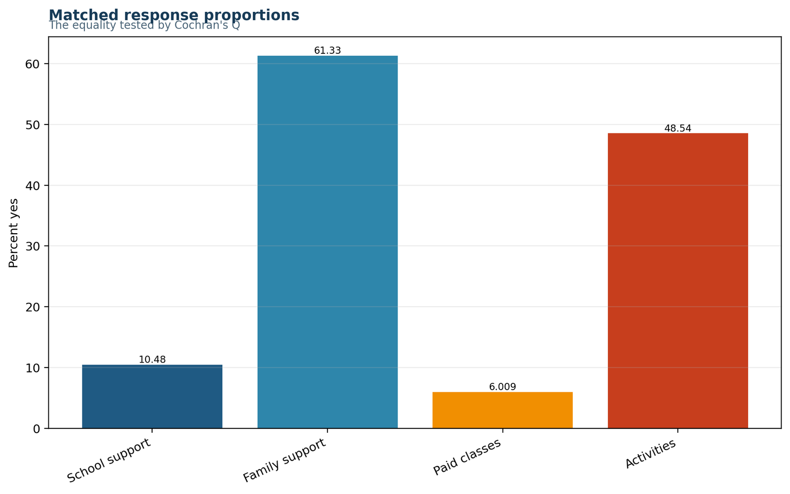
Famsup (61.33%) and activities (48.54%) are much larger than schoolsup (10.48%) and paid (6.01%).
0.1048, 0.6133, 0.0601 and 0.4854.
The unequal percentages provide the substantive reason for the significant result.
Readers often understand the practical pattern better through percentages than raw totals.
Chart 3: Subject response totalsPython
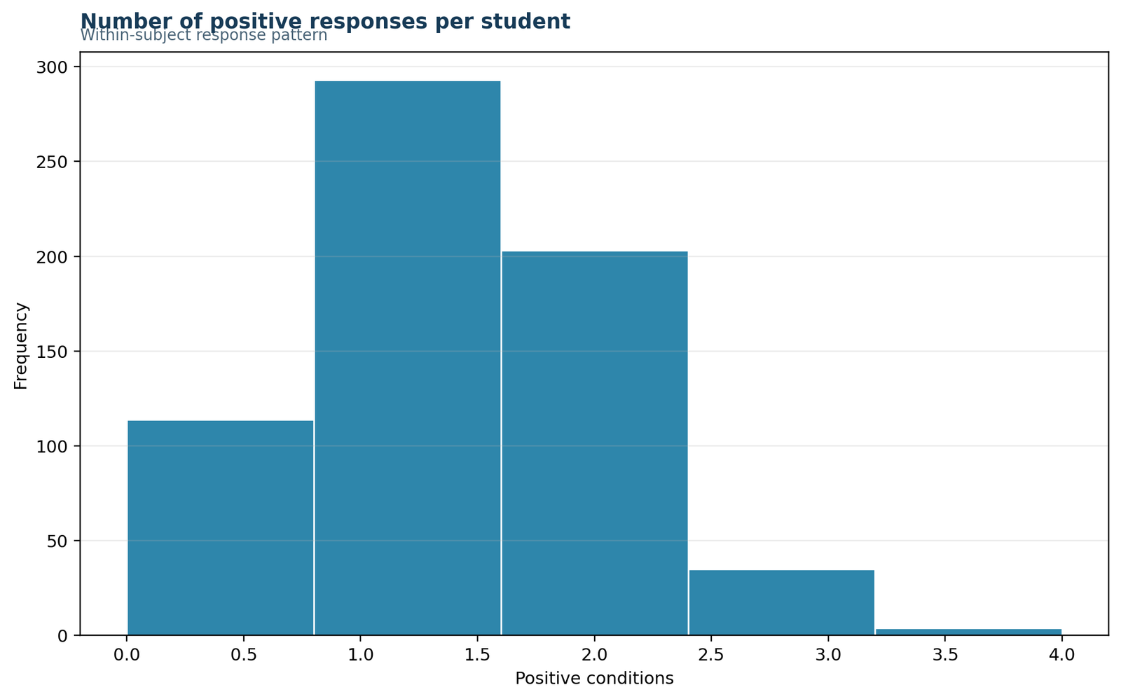
Most students have one or two yes responses, while all-four-yes is rare.
Row totals 0 through 4 occur 114, 293, 203, 35 and 4 times.
This distribution determines ΣRi2, which appears in the Q denominator.
Cochran’s Q is a matched test, so subject-level totals matter.
Chart 4: Pairwise discordancePython
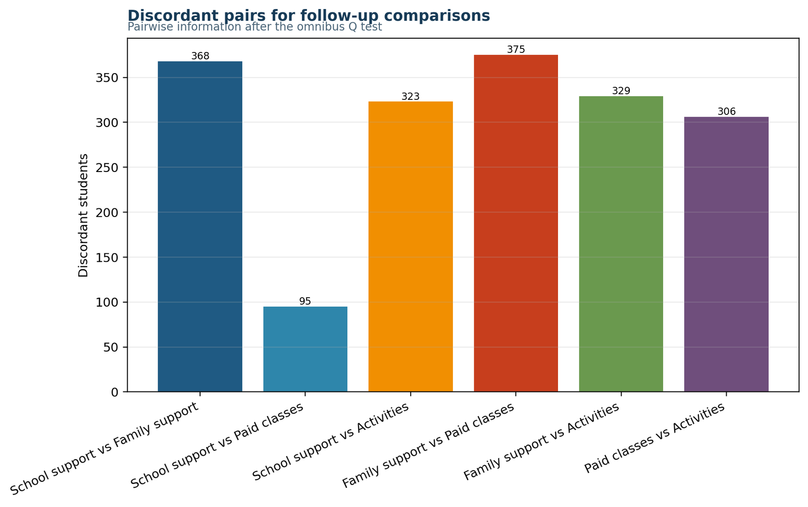
The largest discordance appears for famsup vs paid and paid vs activities.
Examples include famsup-only 367 vs paid-only 8, and activities-only 291 vs paid-only 15.
These imbalances explain why pairwise McNemar follow-ups will be significant.
Discordance, not agreement, drives pairwise matched comparisons.
Chart 5: Pairwise p-valuesPython
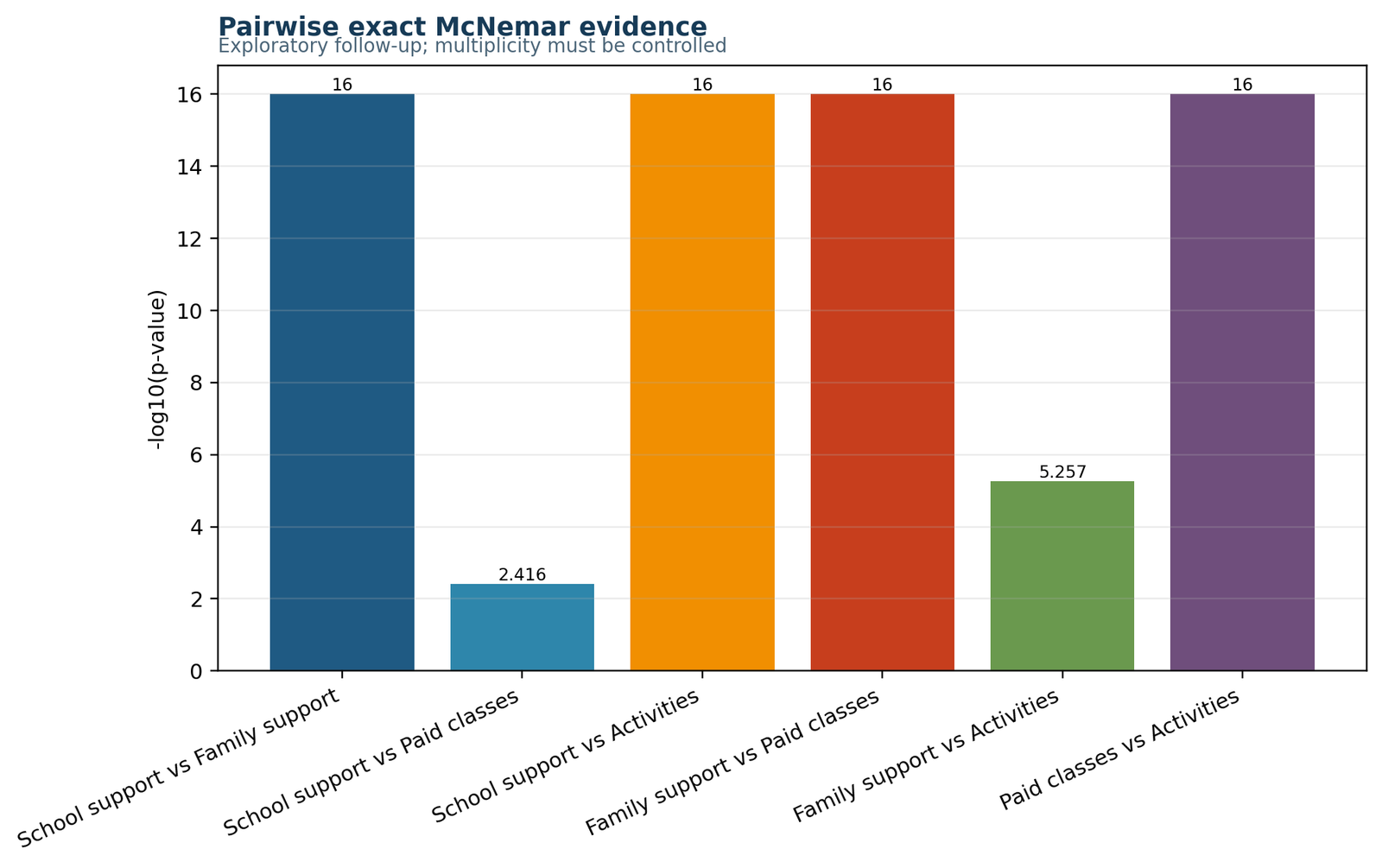
All pairwise comparisons are strongly significant, although their strengths differ.
The least extreme pair is schoolsup vs paid, while the strongest gaps include famsup vs paid and paid vs activities.
The pairwise picture agrees with the large global Q statistic.
This helps move from a global rejection to a clear condition ranking.
Chart 6: Result summaryPython
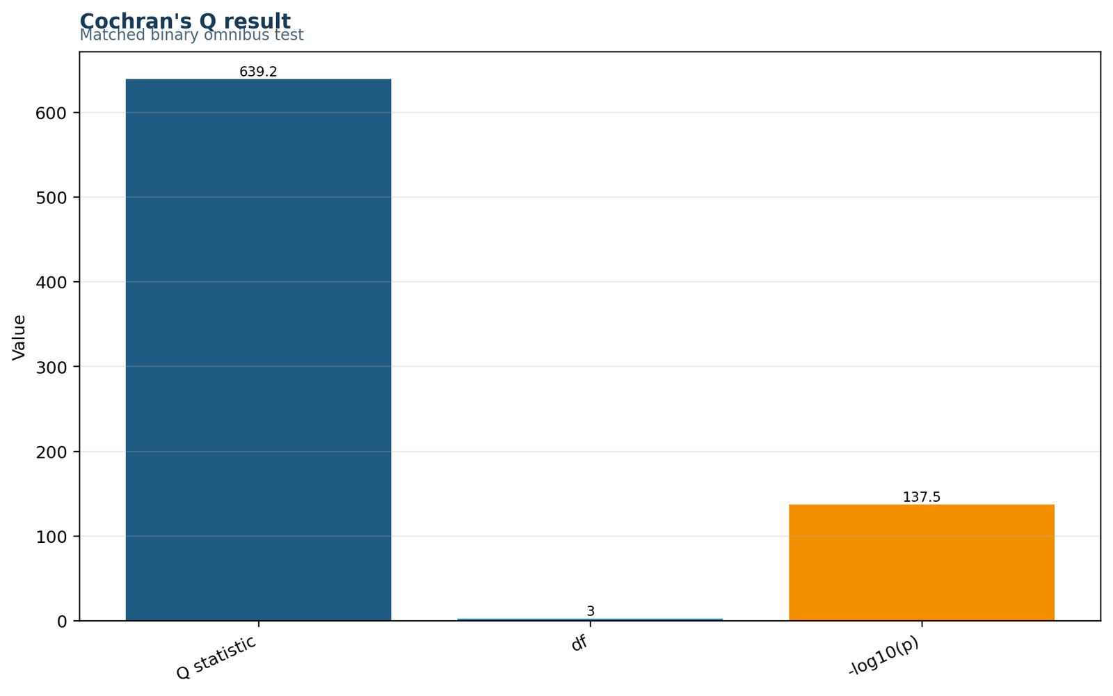
The summary panel consolidates the large Q statistic and effectively zero p-value.
Q = 639.2472, df = 3, p ≈ 3.12 × 10−138.
The equal-probability null is decisively rejected.
This is the clean chart to use in slides or brief result summaries.
R Chart Pairs and Interpretation
The R workflow reproduces the same conclusion but presents the visuals as paired panels. This helps the reader compare raw response counts with proportions, row totals with pattern frequencies, and deviations with the final test decision.
R pair 1: Response counts and response proportions
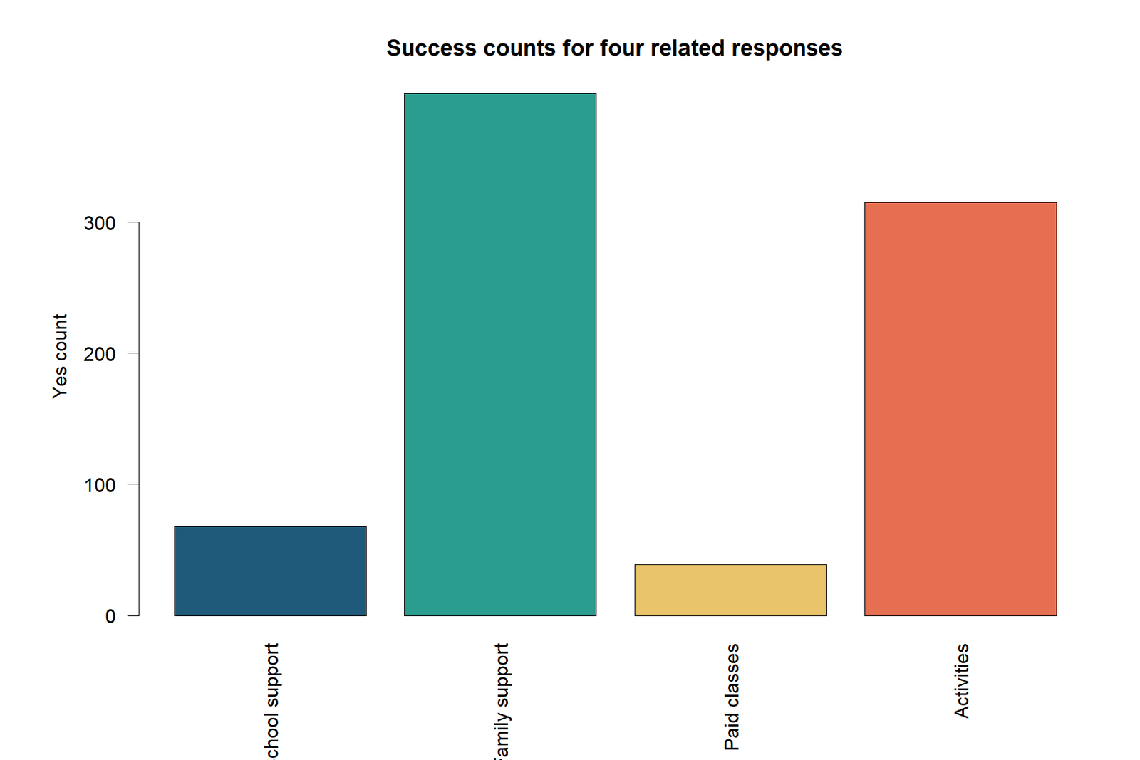
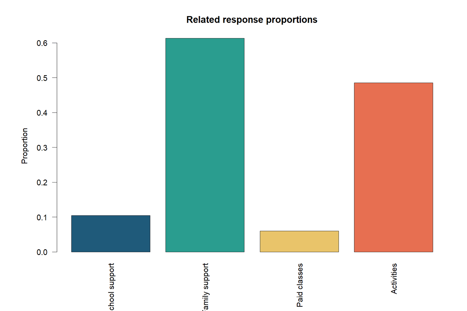
Counts and percentages tell the same story
The count panel shows family support and activities well above school support and paid classes. The proportion panel makes this difference easier to interpret because all four conditions share the same denominator of 649 students.
Strong unequal response probabilities
The equal-probability null would imply similar heights across the four conditions. The visible separation among bars strongly anticipates the significant Cochran’s Q result.
R pair 2: Subject row totals and common response patterns
Most students give one or two yes answers
The row-total distribution is concentrated at 1 and 2. This tells us that agreement is not universal and that there is enough within-student variation for the global repeated-binary comparison to be informative.
Recurring patterns reveal substantive structure
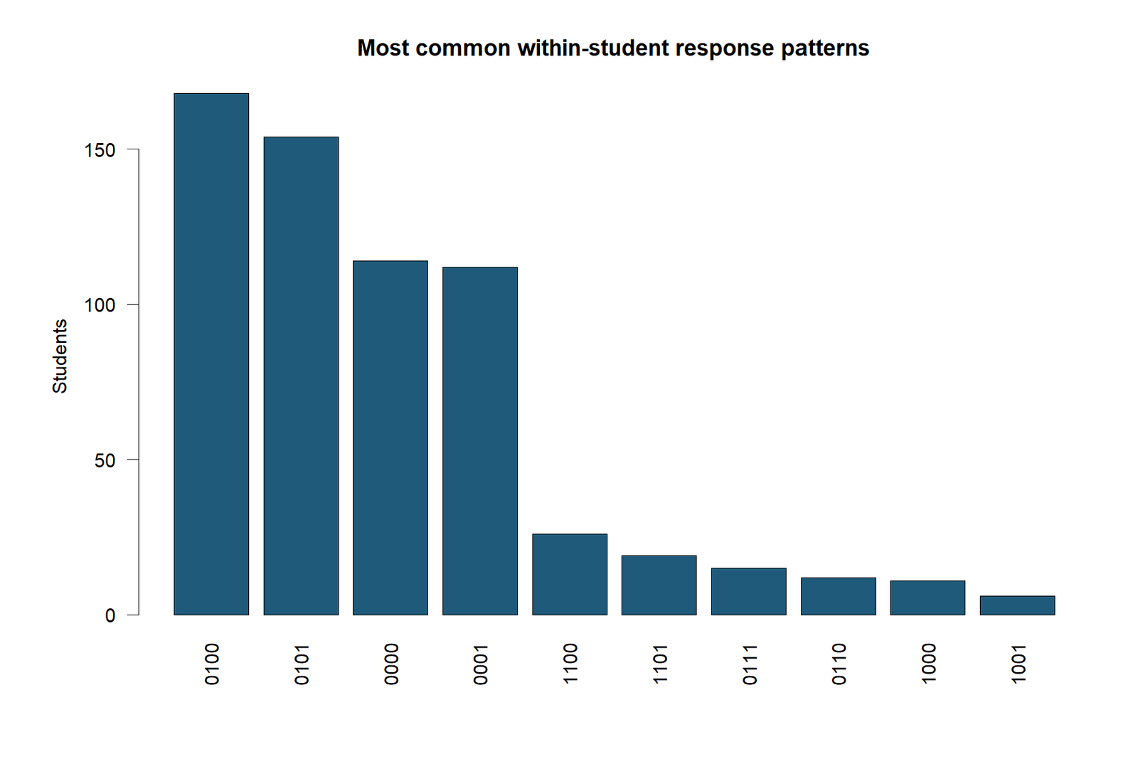
Common patterns such as 0100 (family support only), 0101 (family support plus activities), 0001 (activities only) and 0000 (none) show that the four conditions are not interchangeable.
R pair 3: Column deviation and result summary
Positive and negative deviations are large
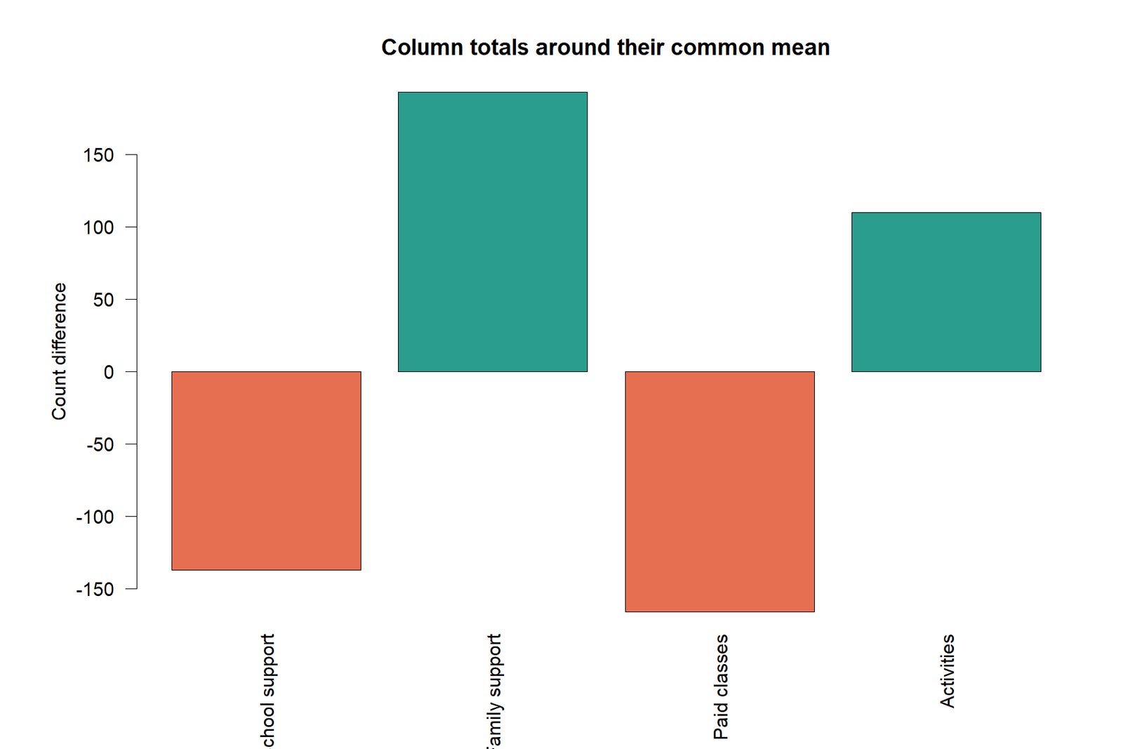
Family support and activities lie above the equal-response expectation, while school support and paid classes lie far below it. The deviations are not small random fluctuations.
The final decision is unambiguous
The summary chart condenses the result to one sentence: Q = 639.2472 with 3 degrees of freedom and an effectively zero p-value, so the null of equal repeated binary probabilities is rejected.
Cochran’s Q Test in Python, R, SPSS and Excel
Python workflow
Use a package or validated implementation that accepts a subject-by-condition binary matrix. The rows must be matched students, not independent groups. Python is also useful for producing post hoc pairwise McNemar analyses and reproducible charts. See categorical data analysis in Python.
- Read the four binary columns.
- Code yes = 1 and no = 0.
- Calculate column totals, row totals, Q and p.
- Create condition, discordance and summary charts.
- Optionally run multiplicity-adjusted pairwise follow-ups.
R workflow
R provides multiple routes for Cochran’s Q Test, including matrix-based and data-frame-based implementations. The key is preserving subject matching and binary coding. See categorical data analysis in R.
- Build a 649 × 4 binary matrix.
- Run the global Q test.
- Compute descriptive proportions.
- Plot row totals and common patterns.
- Follow with pairwise matched tests if needed.
SPSS workflow
SPSS offers Cochran’s Q through the Nonparametric Tests / Legacy Dialogs route and via syntax. This is the correct repeated-binary procedure; do not substitute independent-samples crosstabs. For broader help, see categorical data analysis in SPSS.
- Place the four dichotomous variables in the related-samples test box.
- Confirm yes/no coding.
- Request descriptive summaries and export output.
- Use separate syntax or follow-up routines for pairwise comparisons.
Excel workflow
Excel can reproduce the full calculation transparently. The worked workbook included here shows the data sheet, observed tables, calculations, diagnostics and reporting sheets.
- Compute the four column totals.
- Compute each student’s row total.
- Sum the squared column totals and squared row totals.
- Apply the Q formula directly.
- Use
CHISQ.DIST.RT(Q, k-1)for the p-value.
Code and Software Notes
Python pseudo-code for Cochran’s Q Test
# Read binary columns: schoolsup, famsup, paid, activities
# Recode yes=1, no=0
# Matrix X has shape (649, 4)
column_totals = X.sum(axis=0)
row_totals = X.sum(axis=1)
k = X.shape[1]
T = column_totals.sum()
Q = (k - 1) * (k * (column_totals**2).sum() - T**2) / (k*T - (row_totals**2).sum())
p = chi2_sf(Q, df=k-1)
R pseudo-code for Cochran’s Q Test
# df contains schoolsup, famsup, paid, activities coded 0/1
X <- as.matrix(df[, c("schoolsup","famsup","paid","activities")])
col_totals <- colSums(X)
row_totals <- rowSums(X)
k <- ncol(X)
T <- sum(col_totals)
Q <- (k-1) * (k*sum(col_totals^2) - T^2) / (k*T - sum(row_totals^2))
p <- pchisq(Q, df = k-1, lower.tail = FALSE)
SPSS syntax idea
* Use the related-samples Cochran's Q procedure on the four binary variables.
NPAR TESTS
 /COCHRAN = schoolsup famsup paid activities
 /MISSING ANALYSIS.
Whether you work in Python, R, SPSS or Excel, the logic must remain the same: matched rows, binary coding and a global repeated-response null. If your software treats the four columns as independent groups, the analysis is wrong.
Assumptions, Interpretation Rules and Common Mistakes
Assumptions
- Each row is an independent subject.
- Within a row, the responses are matched or repeated.
- Each condition is dichotomous.
- The same set of conditions is observed for each subject.
- Missing-data handling is defined before testing.
Common mistakes
- Treating related responses as independent groups.
- Using Cochran’s Q for multi-category or continuous outcomes.
- Reporting only the p-value without the four proportions.
- Skipping post hoc logic after a significant global test.
- Forgetting multiplicity adjustment in pairwise follow-up tests.
It is also useful to distinguish Cochran’s Q from chi-square assumptions, because both methods use categorical data but not the same design. Cochran’s Q does not assume independent columns; instead, it explicitly models matched columns. Likewise, it differs from Cochran’s C Test, which is a variance-homogeneity procedure and an entirely different method.
APA Reporting for Cochran’s Q Test
Concise APA sentence
A Cochran’s Q Test showed that the proportion of “yes” responses differed significantly across the four related conditions, Q(3) = 639.25, p < .001. The observed yes proportions were 10.48% for school support, 61.33% for family support, 6.01% for paid classes and 48.54% for activities.
Longer write-up with follow-up note
To compare four matched dichotomous responses measured on the same 649 students, a Cochran’s Q Test was performed. Results indicated a statistically significant difference among the related response probabilities, Q(3) = 639.25, p < .001. Family support (61.33%) and activities (48.54%) were reported much more often than school support (10.48%) and paid classes (6.01%). Because the global test was significant, pairwise matched follow-up comparisons were then examined with multiplicity control.
Students preparing for exams can compare this write-up style with broader reporting guidance in AP Statistics Formula Sheet, AP Statistics exam review and hypothesis testing.
Downloads
R PDF reportR output and chart workflow for the same matched binary analysis.
SPSS PDF outputSPSS related-samples output for Cochran’s Q Test.
Worked Excel analysisTransparent workbook with data, calculations, diagnostics and reporting sheets.
Frequently Asked Questions
What is the null hypothesis of Cochran’s Q Test?
The null states that all related binary conditions have the same probability of a yes response. In the worked example, it says the probabilities for school support, family support, paid classes and activities are equal.
Is Cochran’s Q Test parametric or nonparametric?
It is commonly treated as a nonparametric or distribution-light test for matched binary responses because it does not assume normality of a quantitative outcome.
What is the difference between McNemar and Cochran’s Q?
McNemar compares two related binary responses. Cochran’s Q extends the same matched binary logic to three or more related responses.
Can I use Cochran’s Q Test for independent groups?
No. If the groups are independent, use an independent-samples categorical procedure such as chi-square test of homogeneity or independence, depending on the design.
What should I do after a significant Cochran’s Q result?
Run planned or multiplicity-adjusted pairwise follow-up comparisons, usually McNemar tests, to determine which specific condition pairs differ.
How do I report the result?
State the test, number of conditions, statistic, degrees of freedom, p-value, decision and the observed condition proportions. A concise report is: Cochran’s Q(3) = 639.25, p < .001.
Conclusion
Cochran’s Q Test is the right tool when one set of participants contributes three or more related binary responses. In this worked example, the same 649 students were evaluated on four yes/no conditions. The condition proportions were markedly different, and the global test confirmed that those differences were statistically significant, Q(3) = 639.25, p < .001.
The applied lesson is straightforward: family support and activities are much more common than school support and paid classes in this dataset. The methodological lesson is equally important: matched binary data must be analysed as matched binary data. If you want to strengthen your broader foundation in this area, continue with conditional probability and independence, chi-square calculator, AP Statistics practice exam and AP Statistics FRQ practice.

