
ANOVA Effect Size, Variance Explained, Eta Squared Comparison and Corrected Population Estimate
Omega Squared: Formula, Interpretation, SPSS, Python, R and Excel Guide
Omega Squared, written as ω², is an ANOVA effect size used to estimate how much population-level variance in the dependent variable is explained by a group factor. In practical ANOVA reporting, Omega Squared is often preferred over eta squared because it applies a correction for sampling bias. This guide explains Omega Squared with ANOVA output, Python charts, R validation charts, SPSS workflow, Excel formula, APA wording, common mistakes, downloadable resources, related guides and FAQ schema.
Quick Answer: Omega Squared Result
The worked ANOVA example compared G3 final grade across four studytime groups. The ANOVA result was statistically significant, with F(3, 645) = 15.876 and p = 5.706e-10. This means the studytime groups did not have equal mean G3 scores.
The effect size comparison showed eta squared = 0.069, omega squared = 0.064, and epsilon squared = 0.064. Omega squared is slightly lower than eta squared because it corrects the between-group variance estimate for error. In this output, ω² = 0.064, which means studytime explains about 6.4% of population-level G3 variance and is interpreted as a medium effect.
Final interpretation: Studytime has a statistically significant effect on G3, and the corrected effect size is medium. Omega squared shows that studytime explains about 6.4% of the population-level variance in G3. The effect is meaningful, but most variation in final grade still remains within studytime groups rather than between studytime groups.
Important reporting point: Omega squared is an effect-size estimate, not a replacement for the ANOVA p-value. The p-value shows whether the group difference is statistically supported. Omega squared shows how large the group effect is after correction for bias.
Table of Contents
- What Is Omega Squared?
- Omega Squared Formula
- ANOVA Hypotheses Behind Omega Squared
- Dataset and ANOVA Variables Used
- SPSS Output Interpretation for Omega Squared
- Python Chart-by-Chart Interpretation
- R Chart-by-Chart Validation
- SPSS, R, Python and Excel Workflows
- Code Blocks for Omega Squared
- APA Reporting Wording
- Common Mistakes
- When to Use Omega Squared
- Downloads and Resources
- Related Guides
- FAQs
What Is Omega Squared?
Omega Squared is an ANOVA effect size that estimates the proportion of population variance explained by a factor. It is written as ω². In a one-way ANOVA, it tells how much of the outcome variation is explained by group membership after correcting for the error expected in a sample estimate.
In this worked example, the outcome variable is G3 final grade, and the group factor is studytime. The ANOVA p-value confirms that the studytime means are not equal. Omega squared then answers the more practical question: how large is the studytime effect?
The output gives ω² = 0.064. This means studytime explains about 6.4% of the population-level variation in G3. The result is not small enough to ignore, but it is also not large enough to claim that studytime alone explains most grade differences.
Simple definition: Omega Squared is a corrected ANOVA effect size. It estimates how much real population variance is explained by a factor. In this example, omega squared = 0.064, so studytime explains about 6.4% of G3 variance.
Omega Squared belongs inside a broader ANOVA effect-size workflow. It should be interpreted together with ANOVA Effect Size, Eta Squared, Cohen’s F Formula, F Distribution, Fixed Effects ANOVA, Factorial ANOVA, ANOVA in SPSS, ANOVA in Python, ANOVA in R and ANOVA Assumptions.
Omega Squared Formula
The one-way ANOVA formula for omega squared uses between-group sum of squares, between-group degrees of freedom, within-group mean square and total sum of squares. It corrects the group effect by subtracting an error-based adjustment.
The correction term dfbetween × MSwithin is the reason omega squared is lower than eta squared. It reduces the effect-size estimate so that it better represents the population effect instead of only the sample effect.
Eta Squared Formula
Eta squared is easier to calculate because it divides between-group variation by total variation. In this output, eta squared is 0.069. Omega squared is 0.064, so the corrected estimate is slightly more conservative.
Epsilon Squared Formula
Epsilon squared is another adjusted effect size. In this output, epsilon squared is also 0.064, almost identical to omega squared. This supports the same medium practical interpretation.
| Effect Size | Formula Logic | Value in This Output | Interpretation |
|---|---|---|---|
| Eta squared | Sample variance explained by group. | 0.069 | Slightly larger estimate. |
| Omega squared | Corrected population variance explained by group. | 0.064 | Preferred conservative estimate. |
| Epsilon squared | Alternative adjusted variance explained estimate. | 0.064 | Matches omega squared closely. |
| Cohen’s f | Converted ANOVA effect-size scale. | About 0.27 | Medium practical effect. |
Threshold rule: A common practical rule is that omega squared around 0.01 is small, around 0.06 is medium, and around 0.14 is large. The observed omega squared of 0.064 sits just above the medium reference level.
ANOVA Hypotheses Behind Omega Squared
Omega squared is calculated after the ANOVA model is fitted. The ANOVA hypothesis tests whether group means are equal. Omega squared then reports how much variance the group effect explains.
| Statement | Statistical Rule | Meaning |
|---|---|---|
| Null hypothesis | H0: μ1 = μ2 = μ3 = μ4 | All studytime groups have equal mean G3. |
| Alternative hypothesis | H1: At least one studytime group mean differs | At least one group has a different mean G3. |
| Effect-size question | ω² estimates explained population variance | Studytime explains about 6.4% of population-level G3 variance. |
Decision for this example: The equal-means null hypothesis is rejected because F(3, 645) = 15.876 and p = 5.706e-10. The effect is not only statistically significant; omega squared = 0.064 shows a medium corrected effect size.
Dataset and ANOVA Variables Used
The worked example uses student performance data. The dependent variable is G3 final grade. The factor is studytime, with four groups. The ANOVA compares mean G3 across those four studytime groups and then calculates omega squared from the ANOVA table.
| Variable | Role | Why It Matters for Omega Squared Analysis |
|---|---|---|
| G3 | Dependent variable | The outcome whose variance is being explained. |
| studytime | ANOVA factor | The grouping variable used to explain G3 differences. |
| Studytime group 1 | Group level | Lowest mean G3, about 10.84. |
| Studytime group 2 | Group level | Mean G3 about 12.09. |
| Studytime group 3 | Group level | Highest mean G3, about 13.23. |
| Studytime group 4 | Group level | High mean G3, about 13.06, with wider uncertainty. |
The group mean pattern gives the practical reason why omega squared is not zero. Studytime group 1 is lower than the other groups, and groups 3 and 4 are higher. However, the boxplots show that the groups still overlap. This is why omega squared is medium rather than large.
Before interpreting Omega Squared, it is useful to review Descriptive Statistics, Mean Median and Mode, Standard Deviation, Variance, Confidence Interval, P Value, and Null and Alternative Hypothesis.
SPSS Output Interpretation for Omega Squared
The SPSS output provides the ANOVA table values needed to calculate Omega Squared. SPSS usually reports sums of squares, degrees of freedom, mean squares, F statistic, p-value and eta squared if requested. Omega squared can then be calculated manually from the ANOVA table.
SPSS ANOVA Table Values
| ANOVA Source | Sum of Squares | df | Mean Square | F | p-value | Interpretation |
|---|---|---|---|---|---|---|
| Between groups | 465.078 | 3 | 155.026 | 15.876 | 5.706e-10 | Studytime groups differ significantly. |
| Within groups | 6298.189 | 645 | 9.765 | Residual variation remains within groups. | ||
| Total | 6763.267 | 648 | Total G3 variation in the model. |
SPSS Effect Size Calculation
| Measure | Calculation Basis | Value | Meaning |
|---|---|---|---|
| Eta squared | SS between / SS total | 0.069 | Studytime explains about 6.9% of sample G3 variance. |
| Omega squared | Corrected ANOVA effect-size formula | 0.064 | Studytime explains about 6.4% of population-level G3 variance. |
| Epsilon squared | Alternative adjusted formula | 0.064 | Confirms the adjusted effect-size estimate. |
SPSS Group Mean Context
| Studytime Group | Mean G3 | Interpretation |
|---|---|---|
| Group 1 | 10.84 | Lowest final grade group. |
| Group 2 | 12.09 | Higher than group 1. |
| Group 3 | 13.23 | Highest final grade group. |
| Group 4 | 13.06 | High final grade group with wider uncertainty. |
SPSS Assumption and Residual Context
The variance context chart reports Levene p = 0.3804, which does not show a serious homogeneity-of-variance problem at alpha = .05. The residual charts still show lower-tail departure because some observed G3 scores are far below their fitted group means.
SPSS interpretation summary: The ANOVA is statistically significant, and omega squared shows a medium corrected effect size. Studytime explains about 6.4% of population-level G3 variance. Residual diagnostics should still be reported because the model includes visible lower-tail residual departures.
Python Chart-by-Chart Interpretation
The Python charts below show the complete Omega Squared interpretation workflow. They include group means, group distributions, effect-size comparison, interpretation thresholds, F distribution, variance context, residuals versus fitted values and residual Q-Q diagnostics.
Python Chart 1: Group Means with 95% Confidence Intervals
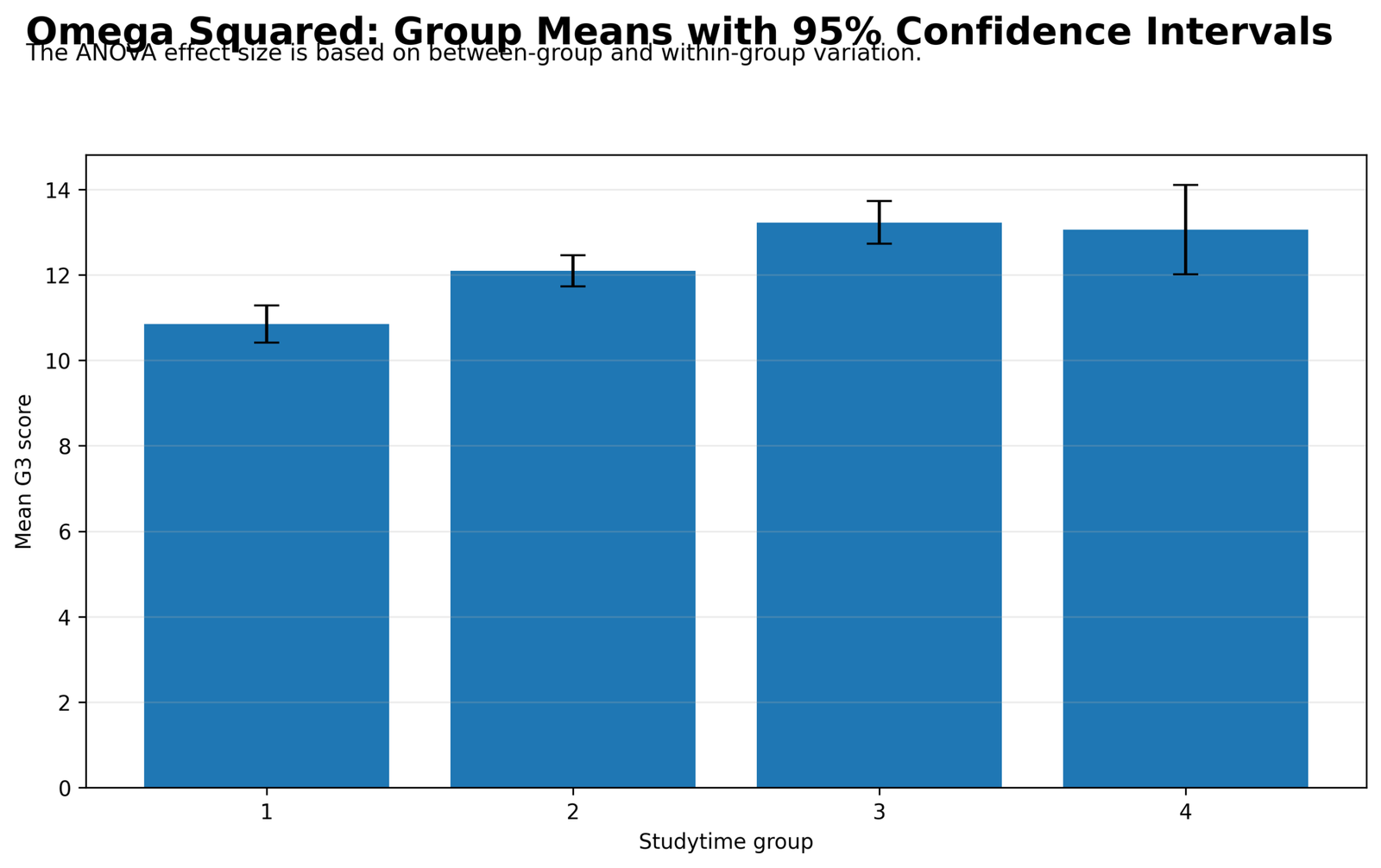
This chart shows the mean G3 score for each studytime group. Group 1 is about 10.84, group 2 is about 12.09, group 3 is about 13.23, and group 4 is about 13.06. The pattern rises strongly from group 1 to group 3, with group 4 remaining high.
The group mean separation is the practical reason the ANOVA is significant. Omega squared then converts that separation into a corrected variance-explained estimate. The confidence interval for group 4 is wider, so its mean is less precise than the larger groups, but it still remains in the high-score range.
Python Chart 2: Distribution by Group
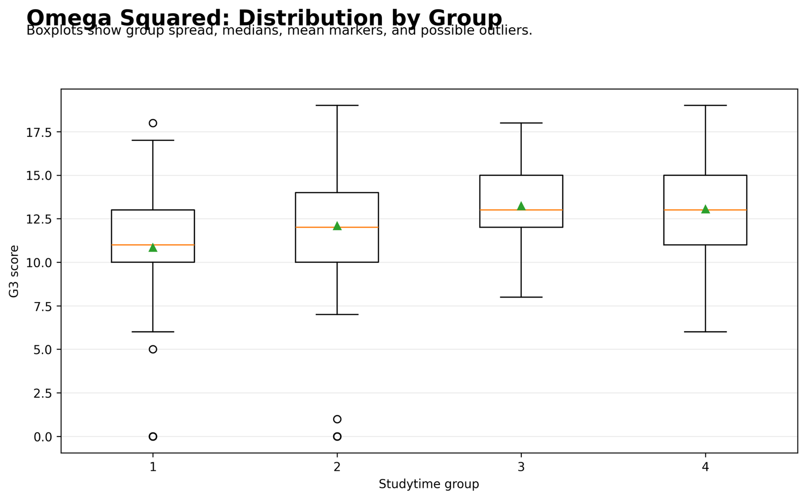
The boxplots show that groups 3 and 4 are centered higher than groups 1 and 2. Group 1 has the lowest central tendency, while group 2 sits between the lowest group and the higher groups.
There are low values in the lower studytime groups, including values near zero. These low observations help explain the residual lower-tail departure seen later. The groups differ, but their distributions still overlap, which supports a medium omega squared result rather than a large one.
Python Chart 3: Effect Size Comparison
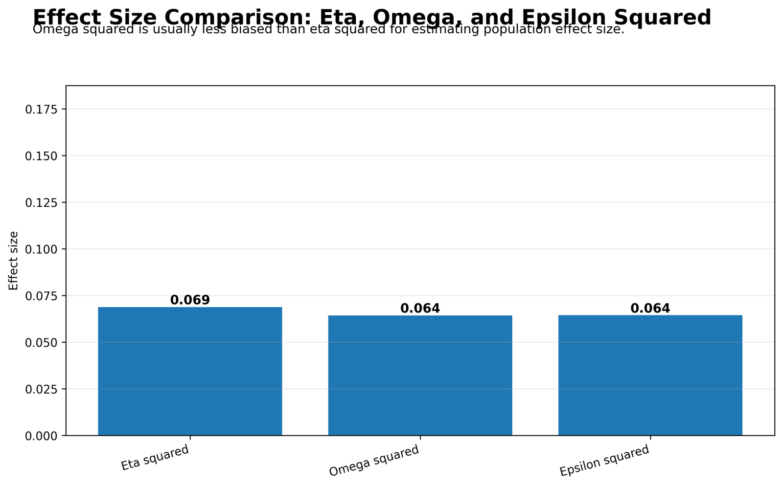
The effect-size comparison chart shows eta squared = 0.069, omega squared = 0.064 and epsilon squared = 0.064. Eta squared is the largest because it does not apply the same correction used by omega squared.
The adjusted measures are nearly identical. This makes the result easy to report: the corrected effect-size estimate is about 0.064. Studytime explains a meaningful part of G3 variance, but it does not dominate the full grade outcome.
Python Chart 4: Omega Squared Interpretation
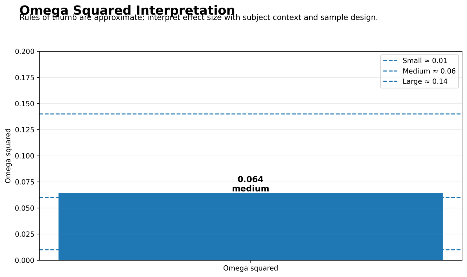
This chart places ω² = 0.064 against the interpretation thresholds. The value is just above the medium reference level around 0.06 and well below the large reference level around 0.14.
The correct interpretation is medium. The chart helps prevent overstatement. The ANOVA p-value is extremely small, but the practical effect size is moderate because much of the G3 variation remains within groups.
Python Chart 5: Observed F Distribution
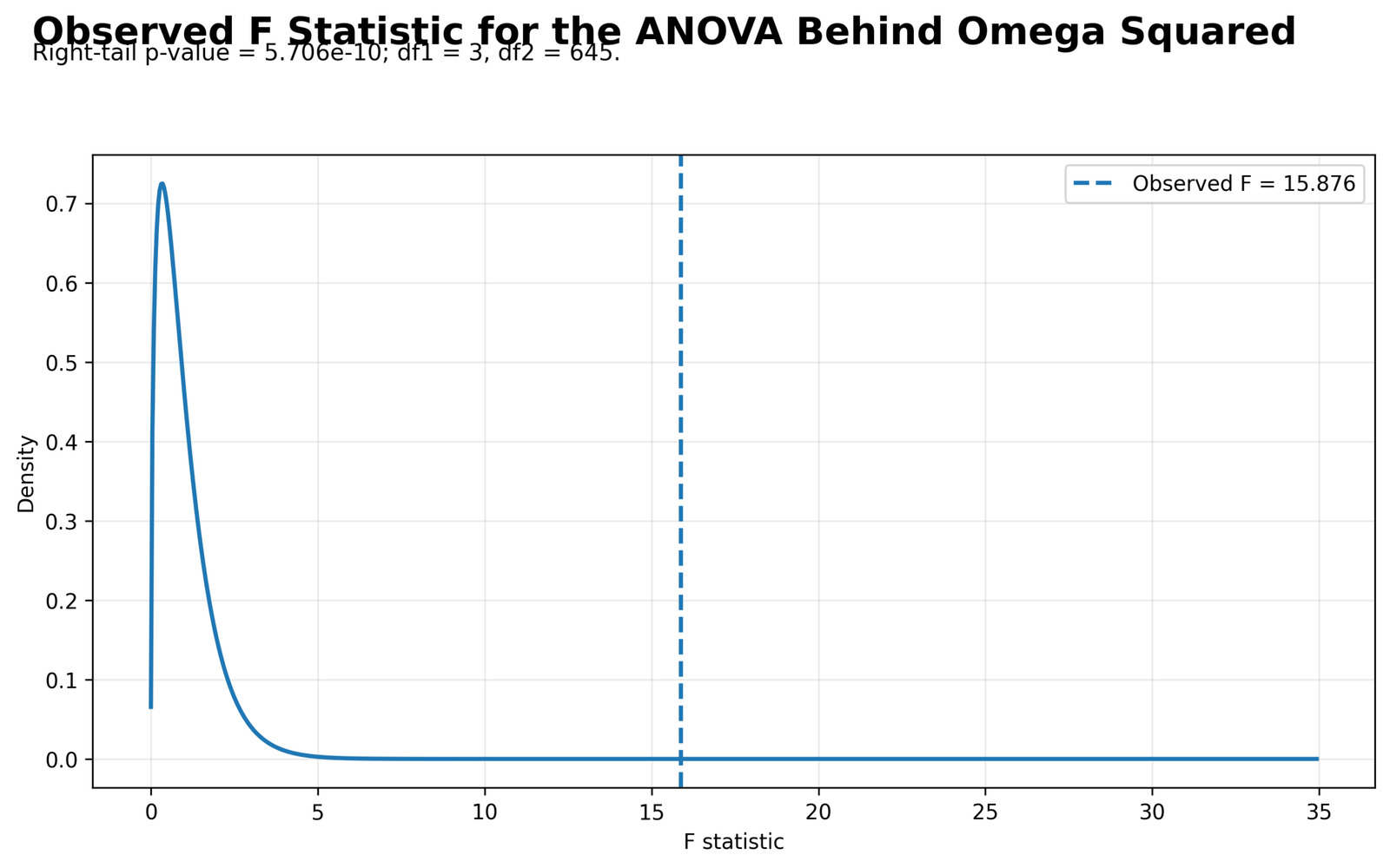
The F distribution chart shows the statistical evidence behind the effect size. The observed value is F = 15.876 with df1 = 3 and df2 = 645. The right-tail p-value is 5.706e-10.
The observed F line is far into the right tail of the distribution. This confirms that the studytime group mean differences are not likely under the equal-means null hypothesis. Omega squared is then reported to describe the size of this significant effect.
Python Chart 6: Variance Context by Group
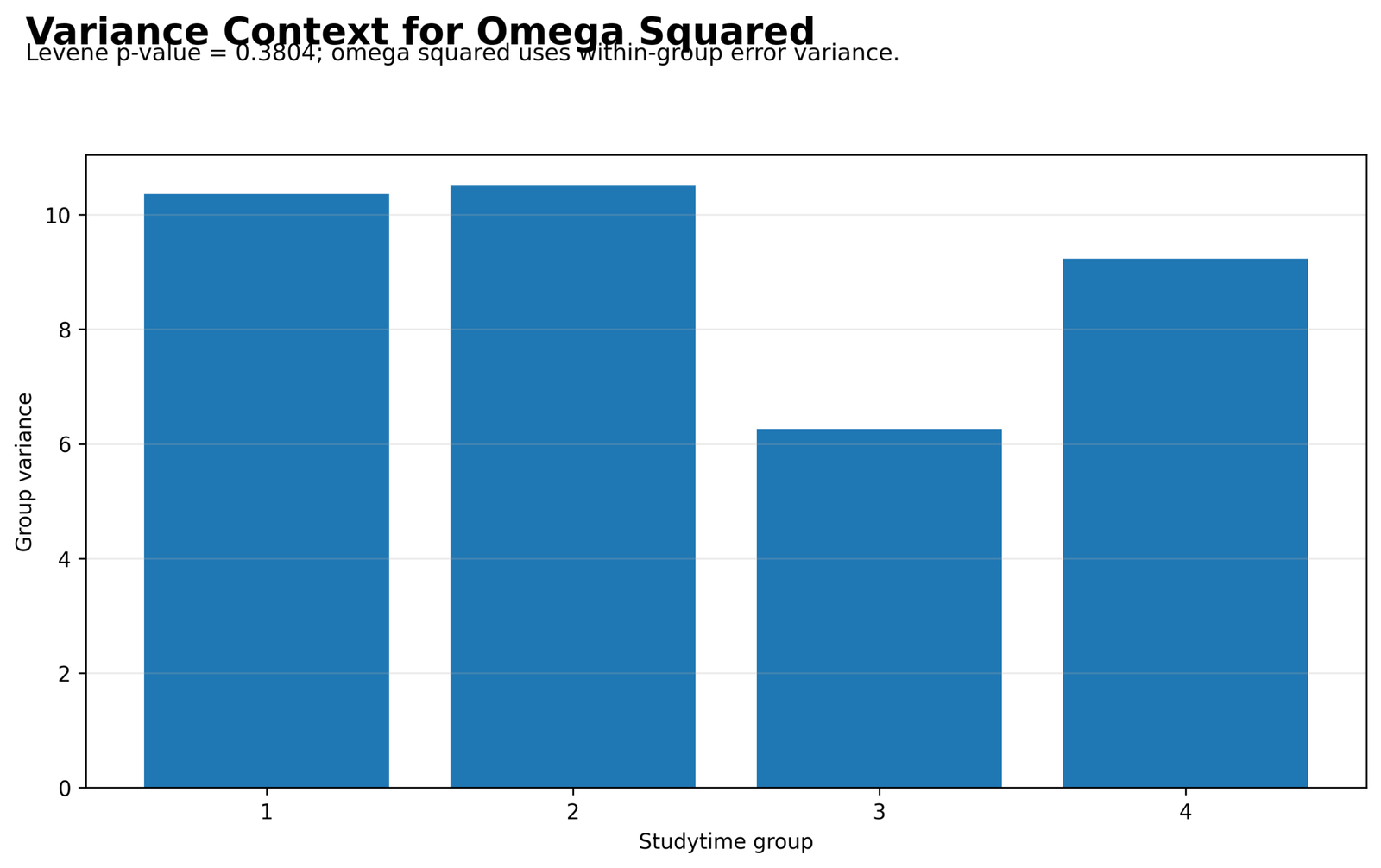
The variance context chart shows that the group variances are not identical. Groups 1 and 2 have larger variance values, group 3 has a smaller variance, and group 4 is between them. The chart reports Levene p = 0.3804.
The Levene result does not show a serious variance violation at alpha = .05. This supports the ANOVA variance assumption more than it challenges it. The chart is still important because omega squared depends directly on the within-group error variance.
Python Chart 7: Residuals vs Fitted Values
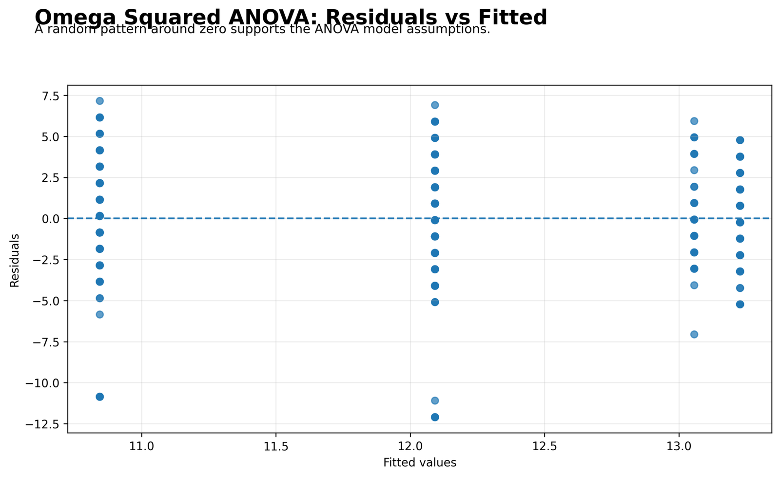
The residuals-versus-fitted chart shows vertical fitted-value bands because the model fits group means. Most residuals are spread around zero, but several negative residuals extend far below the center line.
The lower negative residuals show students whose G3 values were much lower than their fitted group mean. This explains why the model is significant but not perfect. Omega squared is medium because the studytime grouping explains some variance while individual grade variation remains large.
Python Chart 8: Residual Q-Q Plot
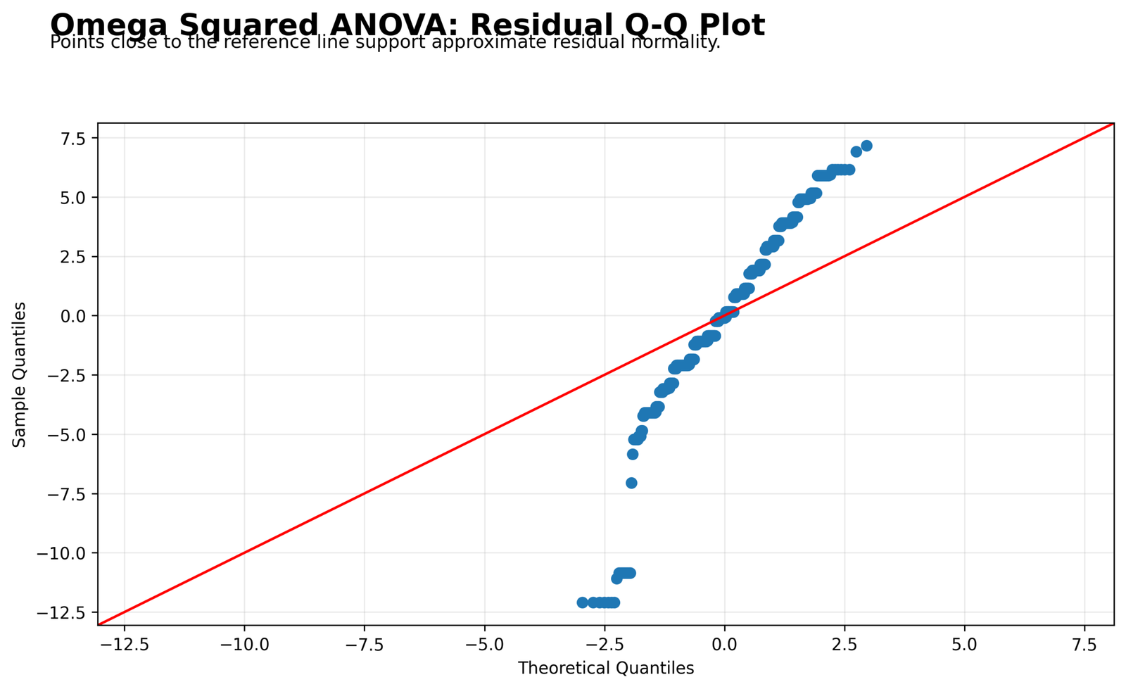
The residual Q-Q plot shows clear lower-tail departure from the reference line. The middle of the residual distribution follows the expected diagonal pattern more closely, while the lower tail bends away strongly.
The diagnostic message is balanced. The ANOVA effect is statistically significant, and omega squared is interpretable, but residual normality is not perfect. The final report should mention this residual pattern instead of claiming that all assumptions were ideal.
R Chart-by-Chart Validation
The R charts validate the Python and SPSS conclusions using a second workflow. The same group mean pattern, effect-size values, F decision, variance context and residual diagnostics appear again. This software-to-software agreement strengthens the omega squared interpretation.
R Chart 1: Group Means with 95% Confidence Intervals
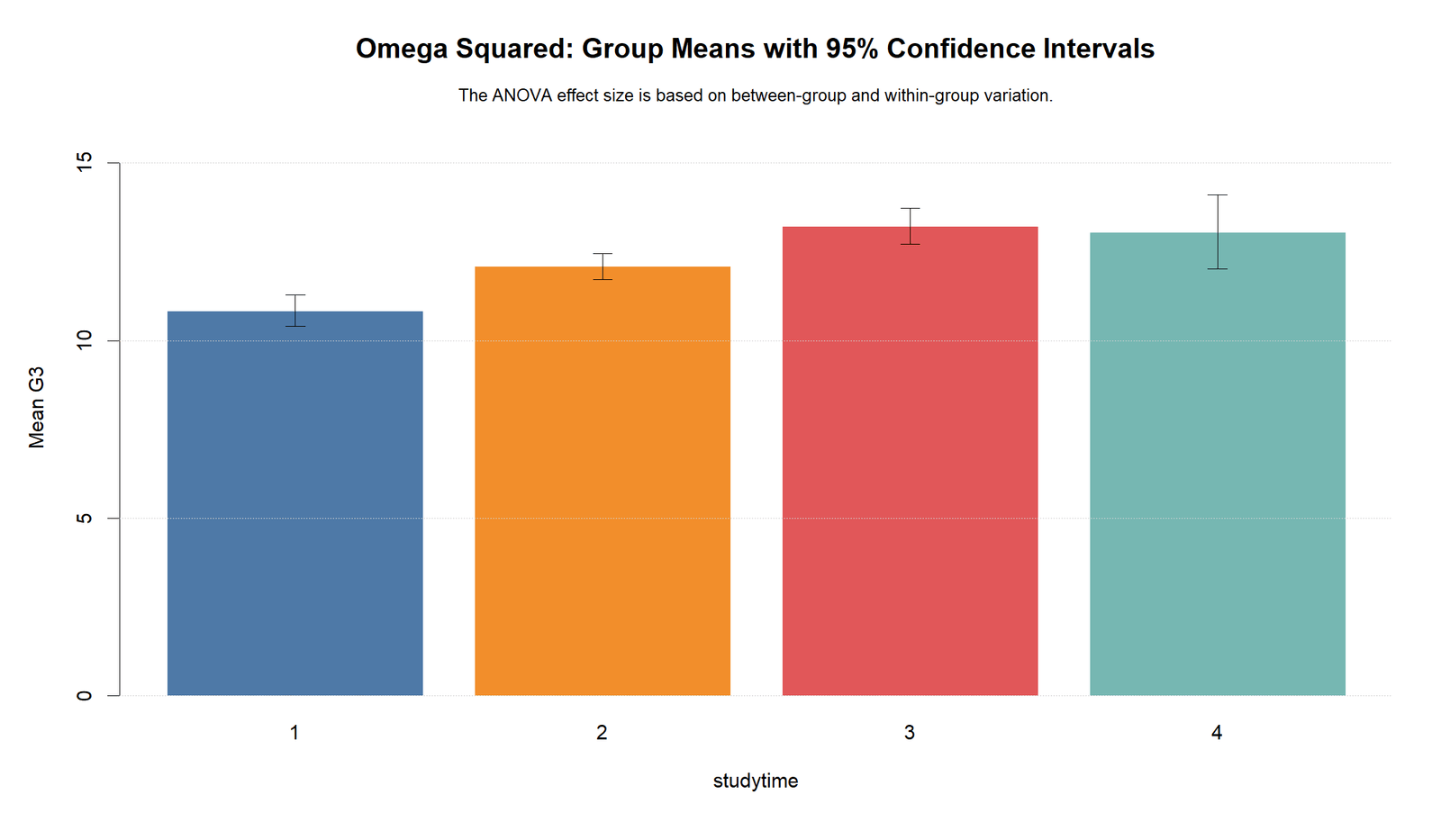
The R group means chart confirms the same group pattern. Studytime group 1 is lowest, group 2 is higher, group 3 is highest, and group 4 remains close to group 3.
This confirms that the group mean pattern is not caused by one software workflow. The same studytime ordering appears in both Python and R, supporting the ANOVA and omega squared interpretation.
R Chart 2: Distribution by Group
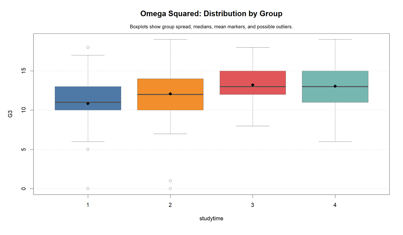
The R boxplots confirm that groups 3 and 4 are centered above groups 1 and 2. Group 1 remains the lowest distribution, and group 2 sits between the low and high groups.
The low observations are visible again. This validates the residual diagnostic interpretation because the same low-score pattern appears before and after model fitting.
R Chart 3: Effect Size Comparison
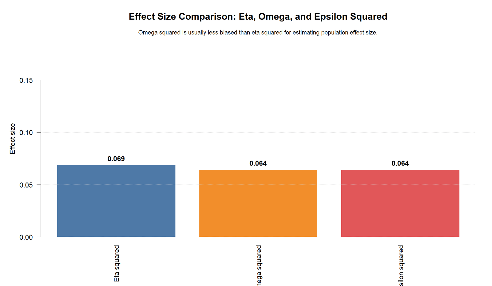
The R effect-size comparison confirms eta squared = 0.069, omega squared = 0.064 and epsilon squared = 0.064. The adjusted effect sizes remain slightly lower than eta squared.
This chart supports using omega squared as the main effect-size estimate. The result is a corrected medium effect rather than only a sample-based variance ratio.
R Chart 4: Omega Squared Interpretation
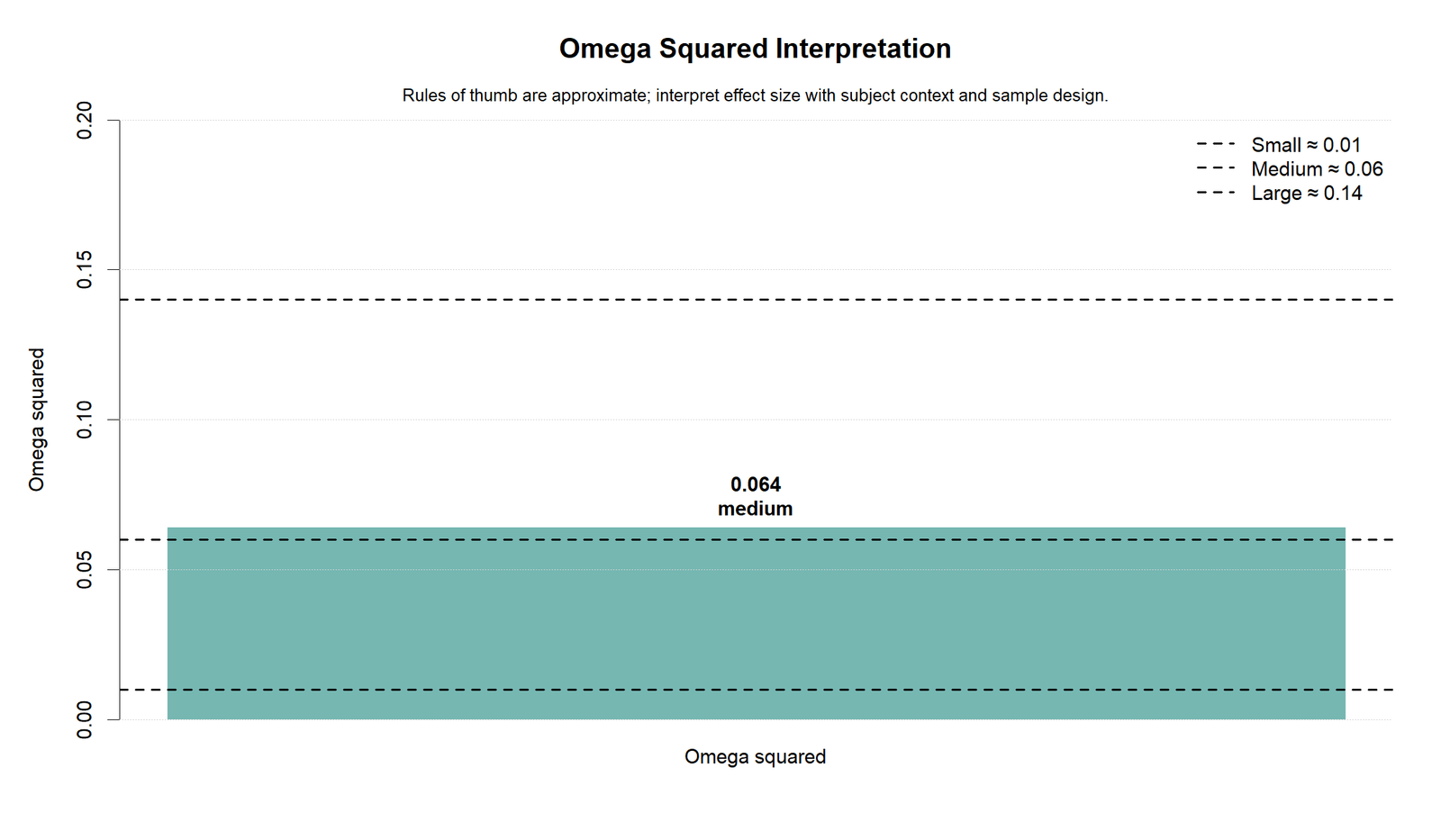
The R interpretation chart confirms the same medium effect-size decision. Omega squared is plotted at 0.064, just above the medium threshold.
This chart is useful for reporting because it converts the numeric effect-size value into a practical conclusion. The result is meaningful, but not large.
R Chart 5: Observed F Distribution
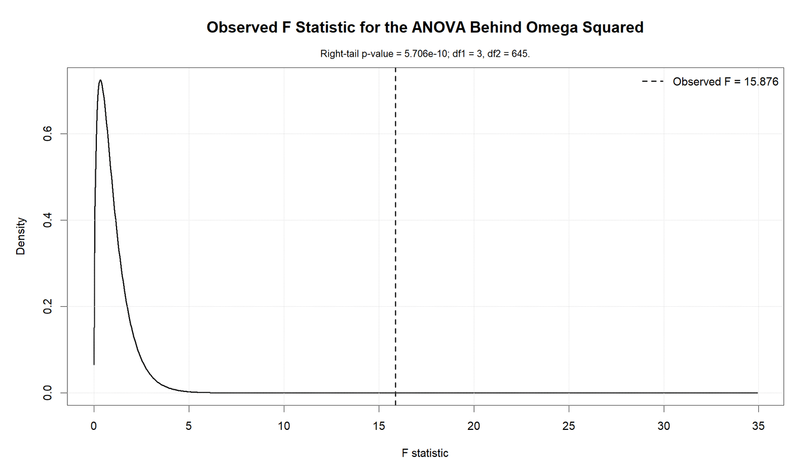
The R F distribution chart confirms the same significance result. The observed F statistic is far to the right of the expected null distribution.
The chart validates the conclusion that studytime groups differ in mean G3. Omega squared is then used to describe the size of that significant ANOVA effect.
R Chart 6: Variance Context by Group
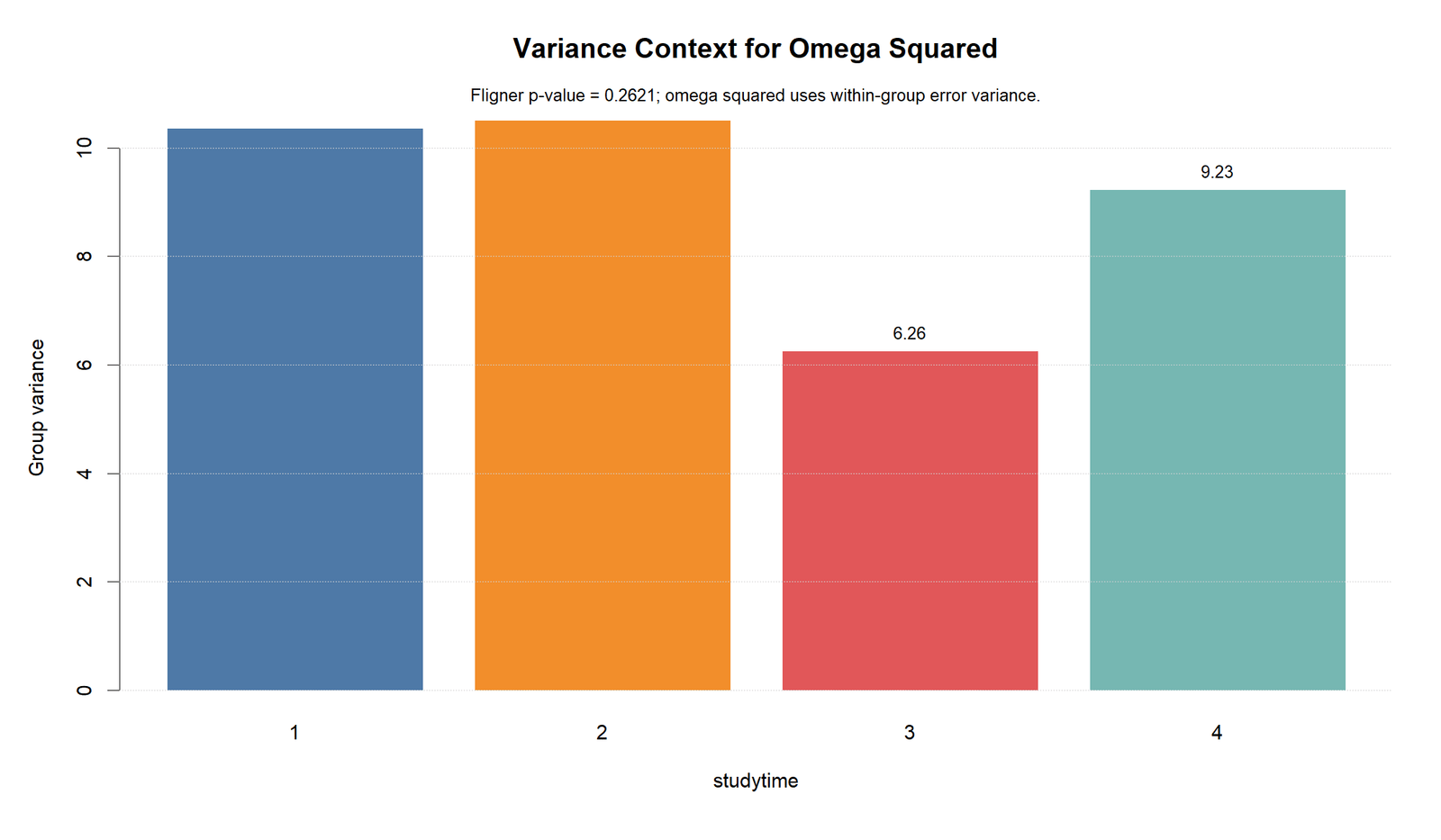
The R variance chart confirms that groups have different spread values. Groups 1 and 2 have larger variances than group 3, while group 4 is in the middle range.
The variance context remains acceptable for the ANOVA interpretation because Levene’s result is not significant at .05. This supports the same assumption discussion given in the Python section.
R Chart 7: Residuals vs Fitted Values
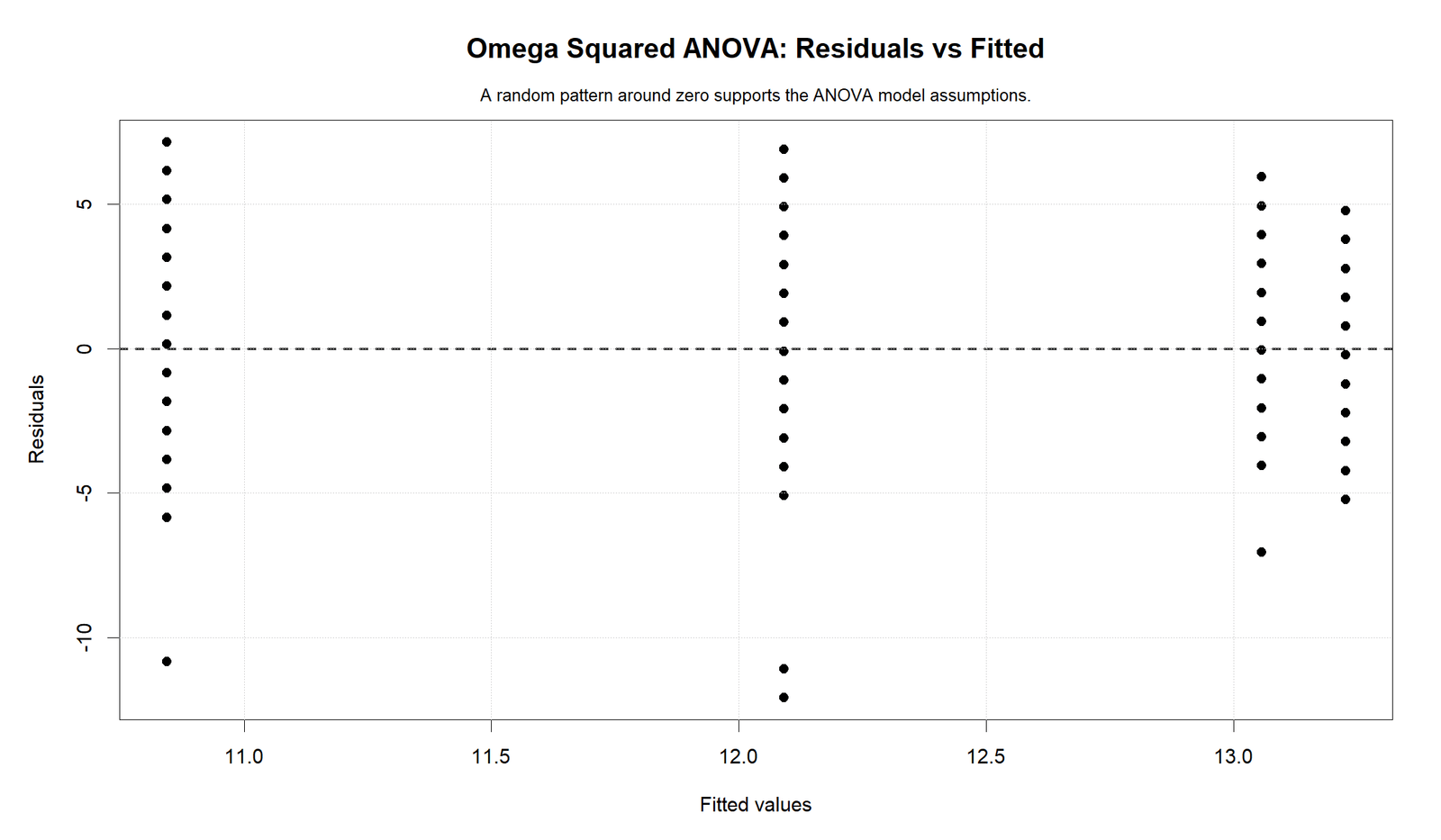
The R residual chart confirms the same fitted-value banding and lower negative residuals. Residuals are centered around zero overall, but several cases fall far below the fitted group means.
This validates the diagnostic warning. The group effect is meaningful, but individual outcomes still vary strongly within groups.
R Chart 8: Residual Q-Q Plot
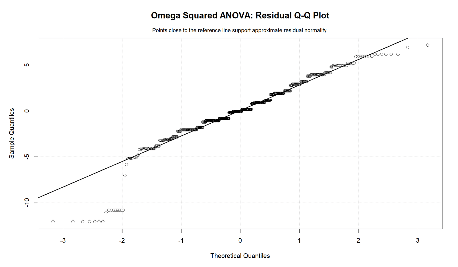
The R Q-Q plot confirms the lower-tail departure already visible in the Python Q-Q plot. The central residuals follow the expected line more closely than the extreme lower tail.
The final diagnostic message remains the same. Omega squared can be reported, but the assumption section should mention that residual normality is approximate rather than perfect.
SPSS, R, Python and Excel Workflows for Omega Squared
The same Omega Squared workflow can be reproduced in SPSS, R, Python and Excel. The core requirement is an ANOVA table with between-group sum of squares, within-group mean square, between-group degrees of freedom and total sum of squares.
SPSS Workflow
| Step | SPSS Menu or Syntax | Purpose |
|---|---|---|
| Open dataset | File > Open > Data | Load the clean dataset. |
| Run ANOVA | Analyze > Compare Means > One-Way ANOVA | Compare G3 across studytime groups. |
| Request descriptives | Options > Descriptive | Get group means, standard deviations and sample sizes. |
| Request variance check | Options > Homogeneity of variance test | Get Levene test output. |
| Read ANOVA table | Between Groups, Within Groups and Total rows | Collect SS, df, MS, F and p-value. |
| Calculate omega squared | Manual formula | Convert ANOVA table into corrected effect size. |
| Export output | File > Export or OUTPUT EXPORT | Save a PDF for reporting and verification. |
R Workflow
| Step | R Action | Purpose |
|---|---|---|
| Read data | read.csv() | Load the dataset. |
| Set factor | as.factor(studytime) | Define studytime as a categorical group factor. |
| Run ANOVA | aov(G3 ~ studytime) | Fit the one-way ANOVA model. |
| Read ANOVA table | summary(model) | Get SS, df, MS, F and p-value. |
| Calculate effect sizes | Manual formula or effectsize package | Calculate eta squared, omega squared and epsilon squared. |
| Check diagnostics | Residuals versus fitted and Q-Q plot | Evaluate assumptions. |
Python Workflow
| Step | Python Action | Purpose |
|---|---|---|
| Read data | pandas.read_csv() | Load G3 and studytime. |
| Fit ANOVA model | ols("G3 ~ C(studytime)") | Fit group mean model. |
| Create ANOVA table | sm.stats.anova_lm() | Get sums of squares, df, F and p-value. |
| Calculate omega squared | Manual formula from ANOVA table | Estimate corrected effect size. |
| Create charts | Group means, effect sizes, F curve and residual diagnostics | Build the visual report. |
| Export report | Save charts and PDF | Create reusable website assets. |
Excel Workflow
| Excel Task | Formula or Tool | Purpose |
|---|---|---|
| Arrange data | Columns for G3 and studytime | Prepare one-way ANOVA layout. |
| Run ANOVA | Data Analysis ToolPak > ANOVA: Single Factor | Generate ANOVA table. |
| Record SS between | Between Groups SS | Needed for omega numerator. |
| Record df between | Between Groups df | Needed for correction term. |
| Record MS within | Within Groups MS | Needed for correction and denominator. |
| Record SS total | Total SS | Needed for denominator. |
| Calculate omega squared | =(SSB-dfb*MSW)/(SST+MSW) | Compute corrected ANOVA effect size. |
Code Blocks for Omega Squared
SPSS Syntax for Omega Squared ANOVA Output
* Omega Squared ANOVA in SPSS.
* Dependent variable: G3.
* Factor: studytime.

TITLE "Omega Squared ANOVA: G3 by Studytime".

ONEWAY G3 BY studytime
  /STATISTICS DESCRIPTIVES HOMOGENEITY
  /MISSING ANALYSIS.

UNIANOVA G3 BY studytime
  /METHOD=SSTYPE(3)
  /INTERCEPT=INCLUDE
  /PRINT=DESCRIPTIVE ETASQ HOMOGENEITY
  /EMMEANS=TABLES(studytime)
  /CRITERIA=ALPHA(.05)
  /DESIGN=studytime.

* Manual omega squared formula from ANOVA table:
* omega squared = (SS_between - df_between * MS_within) / (SS_total + MS_within).

OUTPUT EXPORT
  /CONTENTS EXPORT=VISIBLE
  /PDF DOCUMENTFILE="omega_squared_output.pdf".
Python Code for Omega Squared
import pandas as pd
import statsmodels.api as sm
from statsmodels.formula.api import ols

df = pd.read_csv("dataset.csv")

df["G3"] = pd.to_numeric(df["G3"], errors="coerce")
df["studytime"] = df["studytime"].astype("category")

df_model = df.dropna(subset=["G3", "studytime"]).copy()

# One-way ANOVA
model = ols("G3 ~ C(studytime)", data=df_model).fit()
anova_table = sm.stats.anova_lm(model, typ=2)

print(anova_table)

# Extract ANOVA components
ss_between = anova_table.loc["C(studytime)", "sum_sq"]
df_between = anova_table.loc["C(studytime)", "df"]
ss_within = anova_table.loc["Residual", "sum_sq"]
df_within = anova_table.loc["Residual", "df"]
ms_within = ss_within / df_within
ss_total = ss_between + ss_within

# Effect sizes
eta_squared = ss_between / ss_total
omega_squared = (ss_between - df_between * ms_within) / (ss_total + ms_within)
epsilon_squared = (ss_between - df_between * ms_within) / ss_total

print("Eta squared:", eta_squared)
print("Omega squared:", omega_squared)
print("Epsilon squared:", epsilon_squared)

# Residual diagnostics
df_model["fitted"] = model.fittedvalues
df_model["residual"] = model.resid

print(df_model[["G3", "studytime", "fitted", "residual"]].head())
R Code for Omega Squared
# Omega Squared analysis in R

library(tidyverse)

df <- read.csv("dataset.csv")

df$G3 <- as.numeric(df$G3)
df$studytime <- as.factor(df$studytime)

df_model <- df %>%
  select(G3, studytime) %>%
  drop_na()

# One-way ANOVA
model <- aov(G3 ~ studytime, data = df_model)

summary(model)

anova_table <- summary(model)[[1]]

ss_between <- anova_table["studytime", "Sum Sq"]
df_between <- anova_table["studytime", "Df"]
ss_within <- anova_table["Residuals", "Sum Sq"]
df_within <- anova_table["Residuals", "Df"]
ms_within <- ss_within / df_within
ss_total <- ss_between + ss_within

eta_squared <- ss_between / ss_total
omega_squared <- (ss_between - df_between * ms_within) / (ss_total + ms_within)
epsilon_squared <- (ss_between - df_between * ms_within) / ss_total

eta_squared
omega_squared
epsilon_squared

# Optional package method:
# install.packages("effectsize")
# library(effectsize)
# omega_squared(model)

plot(model)
Excel Formulas for Omega Squared
Step 1:
Run one-way ANOVA using Data Analysis ToolPak.

Step 2:
Record these ANOVA table values:
SS_between = Between Groups Sum of Squares
df_between = Between Groups df
MS_within = Within Groups Mean Square
SS_total = Total Sum of Squares

Step 3:
Calculate eta squared:
=SS_between / SS_total

Step 4:
Calculate omega squared:
=(SS_between - df_between * MS_within) / (SS_total + MS_within)

Step 5:
Calculate epsilon squared:
=(SS_between - df_between * MS_within) / SS_total

Step 6:
Interpret omega squared:
Around 0.01 = small
Around 0.06 = medium
Around 0.14 = large

Example:
Omega squared = 0.064 means studytime explains about 6.4% of population-level G3 variance and is interpreted as a medium effect.
APA Reporting Wording
When reporting Omega Squared, include the ANOVA F statistic, degrees of freedom, p-value, omega squared value and the practical interpretation. Eta squared can be mentioned as a comparison, but omega squared should be identified as the corrected estimate.
APA-style report: A one-way ANOVA showed that mean G3 differed significantly across studytime groups, F(3, 645) = 15.876, p = 5.706e-10. Omega squared indicated a medium corrected effect size, ω² = 0.064, meaning studytime explained about 6.4% of population-level variance in G3. Eta squared was 0.069 and epsilon squared was 0.064. Residual diagnostics showed lower-tail departures, so the result was interpreted with diagnostic caution.
Short reporting version: Studytime had a significant effect on G3, F(3, 645) = 15.876, p < .001. Omega squared was 0.064, indicating a medium ANOVA effect size.
Common Mistakes
| Mistake | Why It Is Wrong | Correct Practice |
|---|---|---|
| Reporting only the ANOVA p-value | The p-value does not show practical effect size. | Report F, p and omega squared together. |
| Confusing eta squared and omega squared | Eta squared is usually less corrected than omega squared. | Use omega squared for a conservative population estimate. |
| Calling 0.064 a large effect | The interpretation chart places 0.064 in the medium range. | Report the result as medium. |
| Ignoring within-group variation | The boxplots show that group distributions still overlap. | Explain that most variation still remains within groups. |
| Ignoring residual diagnostics | The Q-Q plot shows lower-tail departure. | Discuss diagnostics and review Q-Q Plot Normality Check. |
| Using omega squared for power analysis without conversion | Power tools often require Cohen’s f. | Use Cohen’s F Formula when needed. |
When to Use Omega Squared
Use Omega Squared when you run ANOVA and need a corrected estimate of the practical group effect. It is especially useful when you want to avoid overreporting the effect size from eta squared alone.
| Situation | Use Omega Squared? | Reporting Note |
|---|---|---|
| One-way ANOVA with group differences | Yes | Report ω² with F and p-value. |
| Need corrected population effect size | Yes | Omega squared is more conservative than eta squared. |
| Need simple sample variance explained | Eta squared can also be reported | Explain that eta squared is slightly larger. |
| Need power analysis input | Convert to Cohen’s f | Use Cohen’s f formula. |
| Assumptions are weak | Use with caution | Report diagnostics and consider robust ANOVA alternatives. |
Omega squared should be compared with Eta Squared, ANOVA Effect Size, Cohen’s F Formula, F Distribution, Fixed Effects ANOVA, Factorial ANOVA, Balanced ANOVA, Brown Forsythe ANOVA and ANOVA Assumptions.
Downloads and Resources for Omega Squared
Use these resources to reproduce the Omega Squared workflow. The R report and SPSS output PDF are included as verification files. Script and workbook placeholders can be replaced after the final downloadable files are uploaded to the WordPress Media Library.
Download Dataset
Practice dataset with G3 and studytime variables.
Download Omega Squared R Report PDF
R report PDF for group means, effect sizes, F statistic and diagnostics.
Download Omega Squared SPSS Output PDF
SPSS output PDF for ANOVA table and omega squared reporting.
Download Python Script
Python code for ANOVA, eta squared, omega squared, epsilon squared and diagnostics.
Download R Script and Excel Workbook
R workflow and Excel support workbook for omega squared calculations.
FAQs About Omega Squared
What is Omega Squared?
Omega Squared is an ANOVA effect size that estimates the proportion of population variance explained by a factor after correction for bias.
What was omega squared in this example?
Omega squared was 0.064.
How should omega squared = 0.064 be interpreted?
Omega squared = 0.064 is interpreted as a medium effect size using the threshold chart in this example.
What was the ANOVA result behind omega squared?
The ANOVA result was F(3, 645) = 15.876, p = 5.706e-10.
Is omega squared the same as eta squared?
No. Eta squared is a sample variance-explained estimate, while omega squared applies a correction and is usually more conservative.
What was eta squared in this example?
Eta squared was 0.069.
What was epsilon squared in this example?
Epsilon squared was 0.064, very close to omega squared.
Why report omega squared instead of only the p-value?
The p-value shows statistical evidence, while omega squared shows practical effect size. Both are needed for a complete ANOVA report.
Can omega squared be calculated in Excel?
Yes. After obtaining the ANOVA table, calculate omega squared as (SS between − df between × MS within) / (SS total + MS within).
How do I report this omega squared result in APA style?
A concise report is: Studytime had a significant effect on G3, F(3, 645) = 15.876, p < .001, with omega squared = 0.064, indicating a medium effect.

