
Python ANOVA, Statsmodels, Scipy, Group Means, F Test, Residual Diagnostics and Effect Size
ANOVA in Python: One-Way ANOVA, Formula, Code, Assumptions, Charts and Interpretation
ANOVA in Python is used to compare means across three or more groups using Python libraries such as pandas, scipy and statsmodels. This guide explains how to run a one-way ANOVA in Python, how to create an ANOVA table, how to interpret the F statistic, how to check residual assumptions, how to calculate effect size and how to report results in APA style. The worked example compares G3 final grade across four studytime groups and uses Python charts for group means, boxplots, sum of squares, F distribution, residual histogram, residual Q-Q plot and effect size summary.
Quick Answer: ANOVA in Python Result
The worked ANOVA in Python example compares G3 final grade across four studytime groups. The group mean chart shows that the average G3 score rises from the lowest studytime group to the higher studytime groups. The visible means are about 10.844 for group 1, 12.092 for group 2, 13.227 for group 3 and 13.057 for group 4.
The F distribution chart shows an observed F statistic around 15.88, which is far above the critical value around 2.62. This supports rejecting the null hypothesis that all studytime group means are equal. The effect size summary shows eta squared close to .069, meaning studytime explains about 6.9% of the variation in G3. Cohen’s f is around .27, which gives a medium effect-size interpretation.
Final interpretation: The Python ANOVA result shows a statistically significant difference in G3 across studytime groups. The effect is meaningful but not dominant: studytime explains about 6.9% of final-grade variation, while most variation remains inside the studytime groups.
Important reporting point: A good ANOVA in Python report should not stop at the p value. It should include group means, F statistic, degrees of freedom, p value, residual diagnostics and effect size. The charts show that the group effect is significant, the higher studytime groups have higher G3 scores, and the residual plots should still be reviewed before final reporting.
Table of Contents
- What Is ANOVA in Python?
- ANOVA Formula Used in Python
- Null and Alternative Hypothesis
- Dataset and Python Variables Used
- Python Chart-by-Chart Interpretation
- Python Workflow with pandas, scipy and statsmodels
- SPSS, R, Python and Excel Workflows
- Code Blocks for ANOVA in Python
- APA Reporting Wording
- Common Mistakes
- When to Use ANOVA in Python
- Downloads and Resources
- Related Guides
- FAQs
What Is ANOVA in Python?
ANOVA in Python means using Python to test whether three or more group means are statistically different. For a one-way ANOVA, one categorical grouping variable is used to compare a numeric outcome. In this example, studytime is the grouping variable and G3 final grade is the numeric outcome.
Python can run ANOVA in more than one way. The scipy.stats.f_oneway function gives a simple one-way ANOVA F test. The statsmodels workflow gives a fuller ANOVA table with sum of squares, degrees of freedom, F statistic and p value. The statsmodels method is better for tutorials because it makes the ANOVA logic visible.
The Python output in this guide shows more than a table. It includes charts for group means, group spread, sum of squares, the F distribution, residual shape, Q-Q normality and effect size. These visuals help students understand both the statistical result and the assumptions behind the result.
Simple definition: ANOVA in Python tests whether group means differ using Python code. In this example, Python tests whether mean G3 final grade differs across four studytime groups.
Before using ANOVA in Python, it helps to understand Descriptive Statistics, Mean Median and Mode, Standard Deviation, Variance, Standard Error, Confidence Interval, P Value, and Null and Alternative Hypothesis.
ANOVA Formula Used in Python
A one-way ANOVA model can be written as:
Here, Yij is the observed G3 score for student j in studytime group i, μ is the grand mean, τi is the studytime group effect, and εij is the residual error.
ANOVA F Statistic
The F statistic compares between-group variation with within-group variation. In the Python chart, the observed F statistic is about 15.88, while the critical F value is about 2.62. The observed F statistic is much larger than the critical value, so the group means differ statistically.
Eta Squared Formula
Eta squared shows the proportion of total outcome variation explained by the group factor. In this Python ANOVA example, eta squared is about .069, meaning studytime explains about 6.9% of the variation in G3.
| ANOVA Term | Python Meaning | Example in This Guide | Interpretation |
|---|---|---|---|
| Dependent variable | Numeric outcome | G3 final grade | The score being compared across groups. |
| Factor | Categorical predictor | studytime | The grouping variable used in ANOVA. |
| SS between | Explained variation | Studytime variation | Variation due to group mean differences. |
| SS within | Error variation | Within studytime groups | Variation left inside the groups. |
| F statistic | MS between divided by MS within | ≈ 15.88 | Tests whether group means differ. |
| Eta squared | Proportion of variance explained | ≈ .069 | Studytime explains about 6.9% of G3 variation. |
Null and Alternative Hypothesis for ANOVA in Python
The Python ANOVA test compares the mean G3 score across four studytime groups. The null hypothesis says all group means are equal. The alternative hypothesis says at least one group mean is different.
| Hypothesis | Statement | Meaning for This Example |
|---|---|---|
| Null hypothesis | H0: μ1 = μ2 = μ3 = μ4 | All studytime groups have the same mean G3 score. |
| Alternative hypothesis | H1: at least one group mean differs | At least one studytime group has a different mean G3 score. |
| Decision evidence | Observed F ≈ 15.88 is greater than critical F ≈ 2.62 | Reject the null hypothesis. |
| Practical evidence | η² ≈ .069 and Cohen’s f ≈ .27 | The group effect is medium in size. |
Decision for this example: The Python ANOVA result rejects the null hypothesis. Studytime groups do not have equal mean G3 scores, and the effect size indicates a medium practical effect.
Dataset and Python Variables Used
The worked example uses a student performance dataset. The outcome variable is G3 final grade, and the grouping variable is studytime. Python treats G3 as numeric and studytime as a categorical factor. The analysis then compares mean G3 across the four studytime groups.
| Variable or Output | Role | Why It Matters in Python ANOVA | Where It Appears |
|---|---|---|---|
| G3 | Dependent variable | Numeric final-grade score being compared. | Group means, boxplot, residuals and ANOVA table. |
| studytime | Grouping factor | Defines the four groups in the one-way ANOVA. | Group mean chart, boxplot and ANOVA model. |
| Residuals | Model errors | Used to check normality and model fit. | Residual histogram and Q-Q plot. |
| Sum of squares | ANOVA decomposition | Separates explained and unexplained variation. | Sum of squares chart and ANOVA table. |
| Effect size | Practical magnitude | Shows how much studytime matters. | Effect size summary chart. |
Python ANOVA should be interpreted with assumption checks. Helpful related guides include ANOVA Assumptions, Levene Test, Q-Q Plot Normality Check, P-P Plot Normality Check, Shapiro-Wilk Test, Outlier Detection, and Effect Size.
Python Chart-by-Chart Interpretation
The Python charts below show the complete ANOVA workflow: group means, group distributions, sum of squares, F statistic, residual histogram, residual Q-Q plot and effect size summary. These charts should be read together because the ANOVA table alone does not explain the direction, assumptions or practical size of the result.
Python Chart 1: Group Means with 95% Confidence Intervals
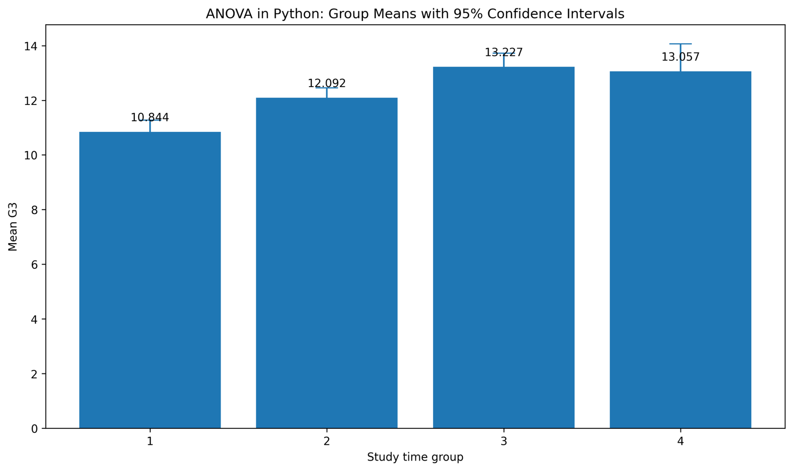
This chart shows the average G3 score for each studytime group. Studytime group 1 has the lowest mean, group 2 is higher, group 3 has the highest mean, and group 4 remains close to group 3. The visible result shows that students in higher studytime categories generally have higher final grades.
The confidence intervals show the uncertainty around each group mean. The first three groups have relatively tighter intervals, while group 4 has a wider interval. This wider interval means the group 4 mean is less precisely estimated than the larger groups, even though its mean remains high.
In the final Python ANOVA report, this chart should introduce the direction of the result. It explains which groups are higher and lower before the F test and p value are reported. The statistical decision still comes from the ANOVA table, but this chart makes the group pattern understandable.
Python Chart 2: Boxplot of G3 by Studytime Group
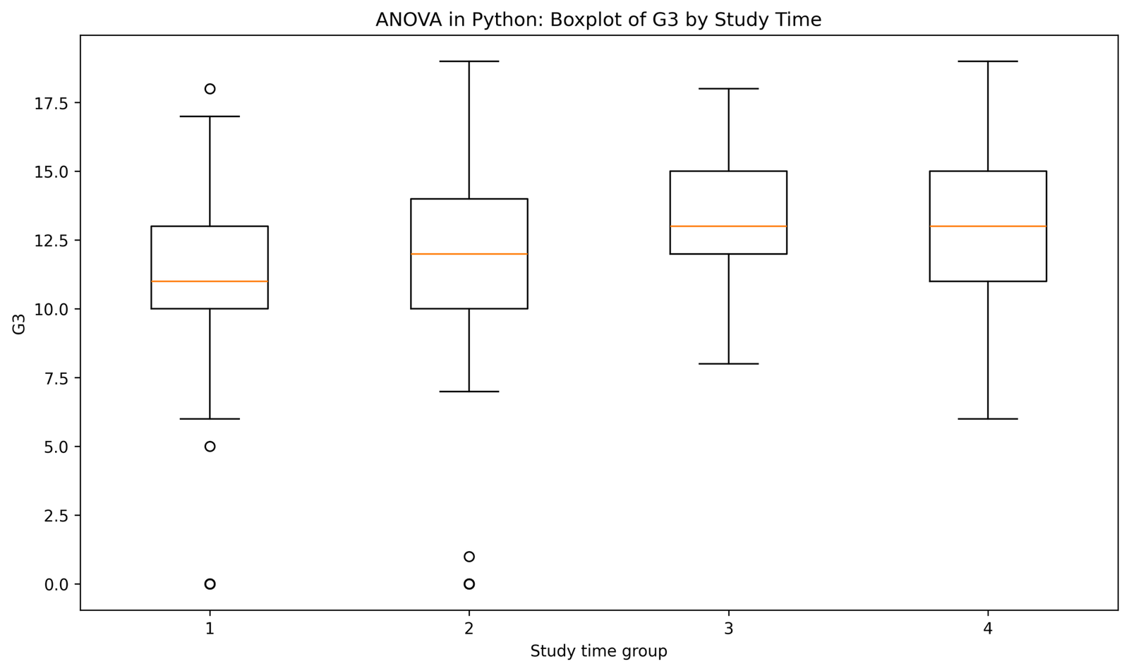
This boxplot shows the full G3 distribution inside each studytime group. The median and center of the distribution are lower in group 1 and higher in groups 3 and 4. This confirms that the group mean chart is not showing a random visual pattern; the distributions themselves also shift upward for the higher studytime categories.
The chart also shows low outliers in the lower studytime groups, especially groups 1 and 2. These low values are important because they also appear later in the residual diagnostics as lower-tail departures. Groups 3 and 4 do not show the same low-score pattern in this figure.
For ANOVA interpretation, the boxplot supports a balanced conclusion. The group centers differ, but the distributions overlap. This explains why the result is significant and medium-sized rather than a complete separation between studytime groups.
Python Chart 3: Sum of Squares Decomposition
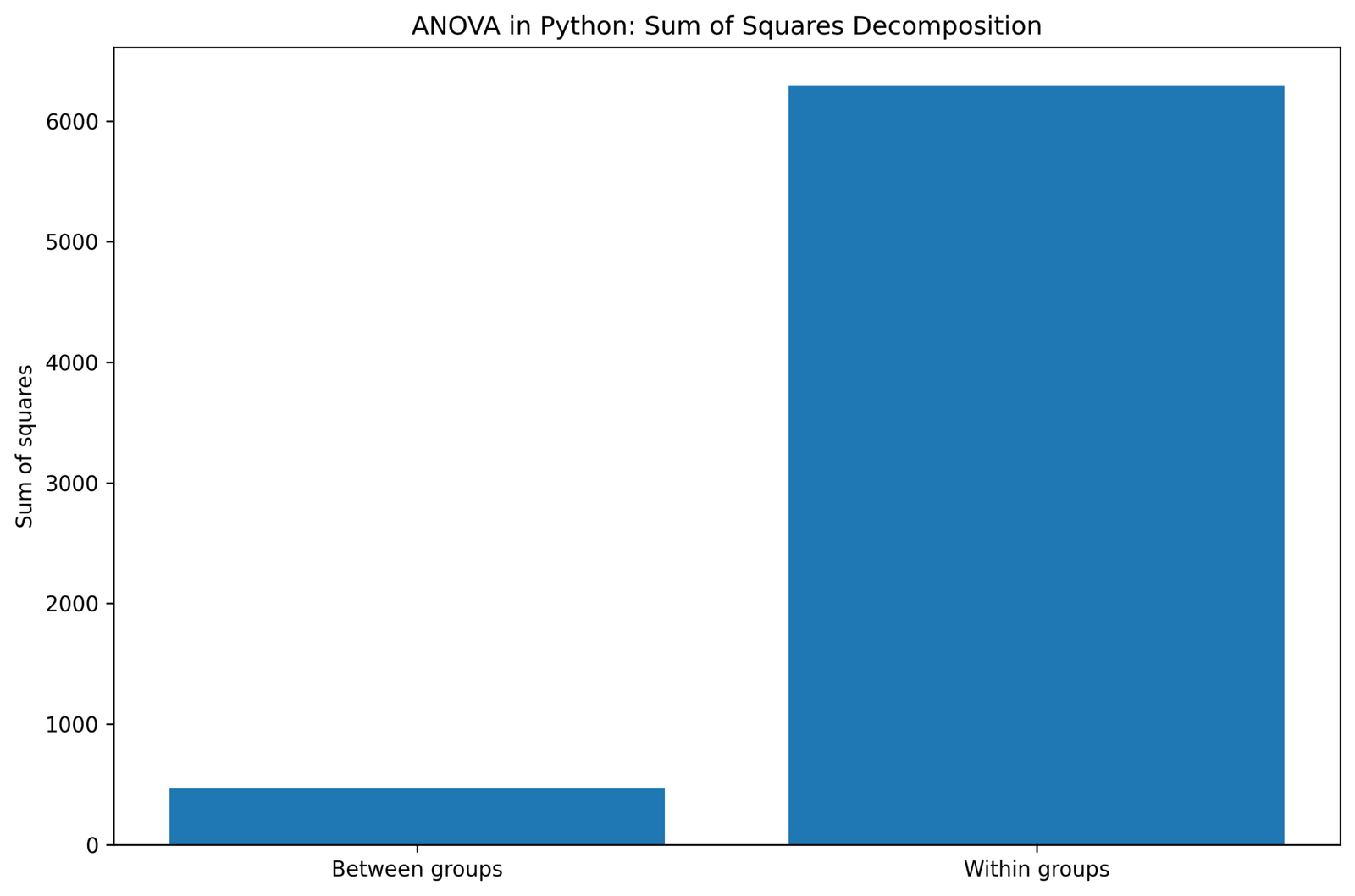
This chart separates the ANOVA variation into between-group variation and within-group variation. The between-group component is the variation explained by studytime group differences, while the within-group component is the variation left inside the groups.
The within-group variation is much larger than the between-group variation. This is expected in real student performance data because grades are affected by many factors beyond studytime. The smaller between-group component is still large enough relative to within-group error to produce a significant F statistic.
In reporting, this chart explains where the ANOVA F statistic comes from. Python does not simply compare the largest mean with the smallest mean; it compares between-group mean square with within-group mean square. The chart also supports the effect-size result because eta squared is calculated from the same sum-of-squares values.
Python Chart 4: F Statistic Distribution Curve
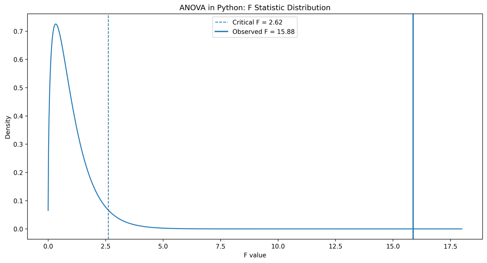
This chart shows the ANOVA F distribution with the observed F statistic and the critical F value marked on the curve. The observed F statistic is around 15.88, while the critical F value is around 2.62.
The observed F value is far to the right of the critical value. This means the group mean differences are too large to be treated as ordinary random within-group variation. The chart supports rejecting the null hypothesis that all studytime group means are equal.
In the Python results section, this chart should be connected directly to the ANOVA table. A correct interpretation is that the studytime effect is statistically significant. The practical meaning should then be explained with effect size, not only with the p value.
Python Chart 5: Residual Histogram
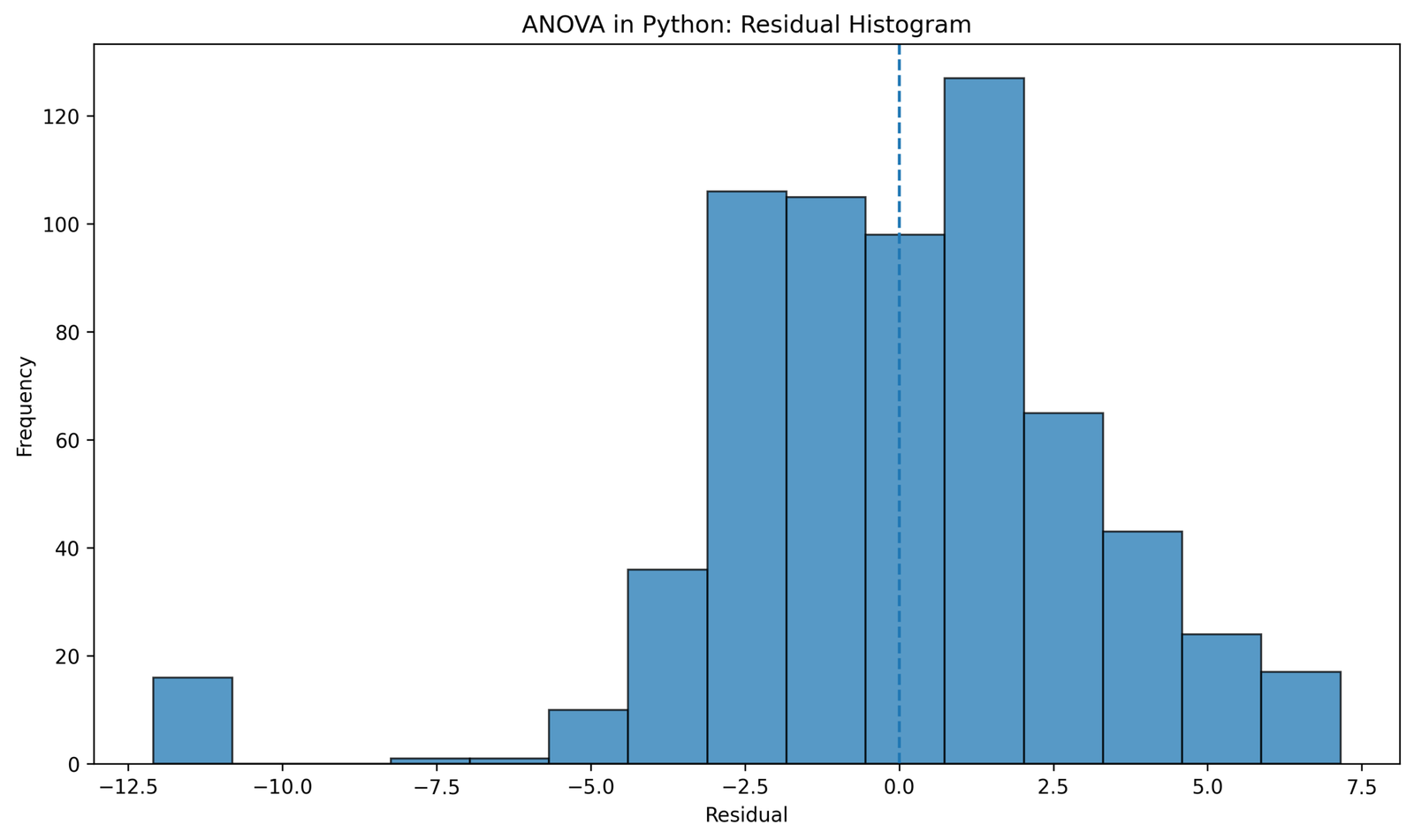
This histogram shows the residuals from the Python ANOVA model. Most residuals are centered around zero, which means the group means capture the center of the G3 scores reasonably well.
The left tail extends farther than the right tail. This means some students scored much lower than the mean predicted for their studytime group. This same issue is visible in the boxplot through low outliers and in the Q-Q plot through lower-tail departures.
In reporting, this chart should be described as mostly centered with lower-tail caution. The residual shape does not erase the significant ANOVA result, but it should be included in the assumption discussion so the report does not claim perfect residual normality.
Python Chart 6: Residual Q-Q Plot
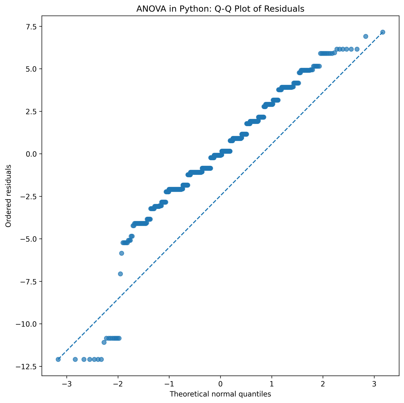
The Q-Q plot shows that the central residuals follow the diagonal line fairly well. This means the middle part of the residual distribution is reasonably close to normal.
The lower-left tail departs from the line, showing that several negative residuals are more extreme than expected under perfect normality. The upper tail also bends away from the line, but the lower-tail behavior is the more important diagnostic pattern in this output.
In the Python ANOVA report, this chart should support a careful assumption statement. The residuals are acceptable in the center, but the lower-tail departures should be mentioned. A formal residual normality test such as Shapiro-Wilk Test, Anderson-Darling Test, Jarque-Bera Test, Lilliefors Test, or Kolmogorov-Smirnov Test can be added if the article needs a formal normality result.
Python Chart 7: Effect Size Summary
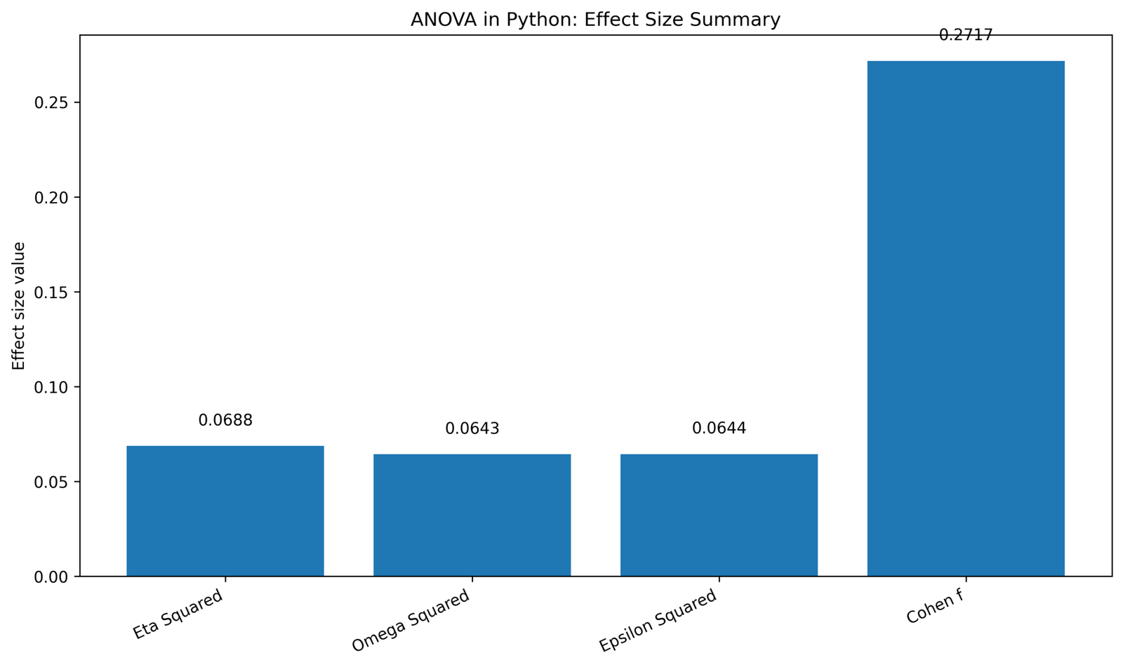
This effect size summary shows the practical size of the studytime effect. Eta squared and partial eta squared are close to .069, while omega squared and epsilon squared are slightly lower, around .064. Cohen’s f is about .27.
The chart labels the effect as medium. This means the studytime difference is not only statistically significant but also meaningful enough to report as a practical result. At the same time, the effect is not huge because most variation in G3 remains within the groups.
In the final article, this chart should be used after the ANOVA table. A complete Python report should say that the result was significant and medium in size, with studytime explaining about 6.9% of G3 variation.
Python Workflow with pandas, scipy and statsmodels
The Python workflow has four main parts: clean the data, run the ANOVA, check assumptions and calculate effect size. pandas prepares the data, scipy can run a quick one-way ANOVA, and statsmodels gives the full ANOVA table.
| Python Step | Library | Purpose | Output |
|---|---|---|---|
| Read dataset | pandas | Load dataset.csv. | DataFrame with G3 and studytime. |
| Clean variables | pandas | Convert G3 to numeric and studytime to category. | Analysis-ready data. |
| Quick ANOVA | scipy | Run one-way ANOVA from grouped arrays. | F statistic and p value. |
| Full ANOVA table | statsmodels | Fit OLS model and extract ANOVA table. | SS, df, F and p. |
| Residual diagnostics | statsmodels and scipy | Check histogram, Q-Q plot and normality. | Residual plots and tests. |
| Effect size | numpy and pandas | Calculate eta squared, omega squared and Cohen’s f. | Practical effect-size interpretation. |
SPSS, R, Python and Excel Workflows for ANOVA
The same ANOVA idea can be run in SPSS, R, Python and Excel. This post focuses on Python, but the workflow table helps readers reproduce the same analysis in other software.
SPSS Workflow
| Step | SPSS Menu | Purpose |
|---|---|---|
| Open data | File > Open > Data | Load G3 and studytime variables. |
| Run ANOVA | Analyze > Compare Means > One-Way ANOVA | Compare G3 means across studytime groups. |
| Request descriptives | Options > Descriptive | Get group means and standard deviations. |
| Check homogeneity | Options > Homogeneity of variance test | Run Levene’s test. |
| Export output | File > Export | Save tables and charts for reporting. |
R Workflow
| Step | R Code | Purpose |
|---|---|---|
| Read data | read.csv("dataset.csv") | Load dataset. |
| Set factor | df$studytime <- as.factor(df$studytime) | Prepare group variable. |
| Run ANOVA | aov(G3 ~ studytime, data=df) | Fit one-way ANOVA. |
| Read table | summary(model) | Get F statistic and p value. |
| Check residuals | plot(model) | Review assumptions. |
Python Workflow
| Step | Python Code | Purpose |
|---|---|---|
| Read data | pd.read_csv("dataset.csv") | Load dataset. |
| Run scipy ANOVA | stats.f_oneway(*groups) | Quick F test. |
| Run statsmodels ANOVA | ols("G3 ~ C(studytime)", data=df) | Fit full model. |
| ANOVA table | sm.stats.anova_lm(model, typ=2) | Extract SS, df, F and p. |
| Effect size | eta_sq = ss_between / ss_total | Report practical magnitude. |
Excel Workflow
| Step | Excel Tool or Formula | Purpose |
|---|---|---|
| Arrange groups | Put each studytime group in a separate column | Prepare data for ANOVA tool. |
| Run ANOVA | Data Analysis ToolPak > ANOVA: Single Factor | Get ANOVA table. |
| Calculate eta squared | =SS_Between/SS_Total | Calculate effect size. |
| Calculate residuals | =Observed - GroupMean | Check model errors. |
| Create charts | Insert > Chart | Visualize group means and residuals. |
Code Blocks for ANOVA in Python
Python Code: Full One-Way ANOVA with statsmodels
import pandas as pd
import numpy as np
import scipy.stats as stats
import statsmodels.api as sm
from statsmodels.formula.api import ols

# Load dataset
df = pd.read_csv("dataset.csv")

# Prepare variables
df["G3"] = pd.to_numeric(df["G3"], errors="coerce")
df["studytime"] = df["studytime"].astype("category")

df_model = df.dropna(subset=["G3", "studytime"]).copy()

# One-way ANOVA model
model = ols("G3 ~ C(studytime)", data=df_model).fit()

# ANOVA table
anova_table = sm.stats.anova_lm(model, typ=2)
print(anova_table)

# Group summaries
group_summary = df_model.groupby("studytime")["G3"].agg(["count", "mean", "std", "var"])
print(group_summary)

# Scipy quick ANOVA
groups = [
    group["G3"].dropna().values
    for name, group in df_model.groupby("studytime")
]

f_stat, p_value = stats.f_oneway(*groups)
print("Scipy F statistic:", f_stat)
print("Scipy p value:", p_value)

# Residuals
df_model["fitted"] = model.fittedvalues
df_model["residual"] = model.resid

# Effect size calculations
ss_between = anova_table.loc["C(studytime)", "sum_sq"]
df_between = anova_table.loc["C(studytime)", "df"]
ss_within = anova_table.loc["Residual", "sum_sq"]
df_within = anova_table.loc["Residual", "df"]
ss_total = ss_between + ss_within
ms_within = ss_within / df_within

eta_squared = ss_between / ss_total
partial_eta_squared = ss_between / (ss_between + ss_within)
omega_squared = (ss_between - df_between * ms_within) / (ss_total + ms_within)
epsilon_squared = (ss_between - df_between * ms_within) / ss_total
cohen_f = np.sqrt(eta_squared / (1 - eta_squared))

print("Eta squared:", eta_squared)
print("Partial eta squared:", partial_eta_squared)
print("Omega squared:", omega_squared)
print("Epsilon squared:", epsilon_squared)
print("Cohen's f:", cohen_f)
Python Code: Assumption Checks
import scipy.stats as stats

# Levene test for homogeneity of variance
levene_stat, levene_p = stats.levene(*groups, center="median")

# Shapiro-Wilk test for residual normality
shapiro_stat, shapiro_p = stats.shapiro(df_model["residual"])

print("Levene statistic:", levene_stat)
print("Levene p value:", levene_p)
print("Shapiro statistic:", shapiro_stat)
print("Shapiro p value:", shapiro_p)

# IQR outlier count by studytime group
def count_iqr_outliers(x):
    q1 = x.quantile(0.25)
    q3 = x.quantile(0.75)
    iqr = q3 - q1
    lower = q1 - 1.5 * iqr
    upper = q3 + 1.5 * iqr
    return ((x < lower) | (x > upper)).sum()

outlier_counts = df_model.groupby("studytime")["G3"].apply(count_iqr_outliers)
print(outlier_counts)
R Code for the Same ANOVA
df <- read.csv("dataset.csv")

df$G3 <- as.numeric(df$G3)
df$studytime <- as.factor(df$studytime)

df_model <- na.omit(df[, c("G3", "studytime")])

model <- aov(G3 ~ studytime, data = df_model)

summary(model)

aggregate(G3 ~ studytime, data = df_model, FUN = mean)

par(mfrow = c(2, 2))
plot(model)
SPSS Syntax for the Same ANOVA
* One-way ANOVA equivalent to Python model.
* Dependent variable: G3.
* Grouping factor: studytime.

TITLE "One-Way ANOVA: G3 by Studytime".

ONEWAY G3 BY studytime
  /STATISTICS DESCRIPTIVES HOMOGENEITY
  /MISSING ANALYSIS.

UNIANOVA G3 BY studytime
  /METHOD=SSTYPE(3)
  /INTERCEPT=INCLUDE
  /PRINT=DESCRIPTIVE ETASQ HOMOGENEITY
  /CRITERIA=ALPHA(.05)
  /DESIGN=studytime.

OUTPUT EXPORT
  /CONTENTS EXPORT=VISIBLE
  /PDF DOCUMENTFILE="ANOVA-in-Python-Equivalent-SPSS-Output.pdf".
Excel Formulas for ANOVA in Python Results
Group mean:
=AVERAGE(group_range)

Group standard deviation:
=STDEV.S(group_range)

Total sum of squares:
=SS_Between + SS_Within

Eta squared:
=SS_Between / SS_Total

Omega squared:
=(SS_Between - df_Between * MS_Within) / (SS_Total + MS_Within)

Cohen's f:
=SQRT(EtaSquared / (1 - EtaSquared))

Residual:
=Observed_G3 - Group_Mean

ANOVA table:
Data > Data Analysis > ANOVA: Single Factor
APA Reporting Wording
When reporting ANOVA in Python, include the dependent variable, grouping factor, group means, F statistic, degrees of freedom, p value, effect size and assumption checks. Python output should be translated into readable statistical reporting, not copied as raw code output only.
APA-style report: A one-way ANOVA was conducted in Python to compare G3 final grade across four studytime groups. The group means increased from the lowest studytime group to the higher studytime groups. The ANOVA result was statistically significant, F(3, 645) ≈ 15.88, p < .001. The effect size was medium, η² ≈ .069, indicating that studytime explained approximately 6.9% of the variance in G3. Residual diagnostics were reviewed using a histogram and Q-Q plot before final interpretation.
Short reporting version: The Python one-way ANOVA showed a significant studytime effect on G3, F(3, 645) ≈ 15.88, p < .001, η² ≈ .069, with a medium effect-size interpretation.
Common Mistakes
| Mistake | Why It Is Wrong | Correct Practice |
|---|---|---|
| Using only scipy and not reading group means | scipy gives F and p but not a full interpretation. | Use pandas summaries and statsmodels ANOVA table. |
| Reporting only p value | The p value does not show practical size. | Report eta squared, omega squared or Cohen’s f. |
| Ignoring residual diagnostics | ANOVA assumptions still matter in Python. | Check residual histogram and Q-Q plot. |
| Treating studytime as numeric when it should be categorical | ANOVA compares groups, not a continuous slope. | Use C(studytime) in statsmodels. |
| Forgetting post hoc tests | ANOVA says at least one group differs, not which exact pairs differ. | Use Tukey HSD or planned comparisons after significant ANOVA. |
| Ignoring unequal variance | Variance problems can affect ordinary ANOVA. | Check Levene Test, Brown-Forsythe Test or Welch-style alternatives. |
When to Use ANOVA in Python
Use ANOVA in Python when you have one numeric outcome and one or more categorical group variables. A one-way ANOVA is used when there is one categorical factor. A two-way ANOVA is used when there are two categorical factors. Repeated measures ANOVA is used when the same subjects are measured repeatedly.
| Research Situation | Python Method | Example |
|---|---|---|
| One numeric outcome and one group factor | One-way ANOVA | G3 by studytime. |
| One numeric outcome and two group factors | Two-way ANOVA | G3 by school and studytime. |
| Same subjects measured repeatedly | Repeated measures ANOVA | Scores across repeated time points. |
| Group comparison with covariate | ANCOVA | G3 by school after adjusting for G2. |
| Only two independent groups | T test | GP versus MS school comparison. |
For related mean-comparison tutorials, see T Test vs ANOVA, ANOVA Assumptions, ANCOVA, Two Sample T Test, Independent Samples T Test, Welch’s T Test, and T Test in Python.
Downloads and Resources for ANOVA in Python
Use these resources to reproduce the ANOVA in Python workflow. Replace placeholder links with final hosted dataset, Python script, SPSS syntax, R script and Excel workbook URLs after uploading them to WordPress Media Library.
Download Dataset
Practice dataset with G3 and studytime variables.
Download Python Script
Python code for one-way ANOVA, assumption checks, charts and effect size.
Download R Script
R validation workflow for the same ANOVA model.
Download Excel Workbook and SPSS Syntax
Excel formulas and SPSS equivalent workflow for comparison.
FAQs About ANOVA in Python
What is ANOVA in Python?
ANOVA in Python is a mean-comparison test run with Python libraries such as scipy and statsmodels. It tests whether three or more group means are statistically different.
How do I run one-way ANOVA in Python?
Use scipy.stats.f_oneway for a quick ANOVA or statsmodels.formula.api.ols with sm.stats.anova_lm for a full ANOVA table.
What is the best Python library for ANOVA?
scipy is useful for a quick F test, while statsmodels is better for a complete ANOVA table with sum of squares, degrees of freedom, F statistic and p value.
How do I interpret ANOVA results in Python?
Read the F statistic and p value to decide whether group means differ. Then read the group means and effect size to explain the direction and practical size of the result.
What does F statistic mean in Python ANOVA?
The F statistic compares between-group variation with within-group variation. A larger F statistic means group means differ more strongly relative to within-group error.
How do I calculate eta squared in Python?
Eta squared is calculated as SS_between / SS_total. In this example, eta squared is about .069, meaning studytime explains about 6.9% of G3 variation.
Do I need residual checks for ANOVA in Python?
Yes. Use a residual histogram, residual Q-Q plot, residuals versus fitted values and variance checks such as Levene’s test before final reporting.
Can I run ANOVA in Python with pandas?
pandas prepares and summarizes the data, but scipy or statsmodels should be used to run the ANOVA test itself.
What should I report after ANOVA in Python?
Report group means, F statistic, degrees of freedom, p value, effect size and assumption-check results.
What is the APA wording for ANOVA in Python?
A concise report is: A one-way ANOVA in Python showed a significant studytime effect on G3, F(3, 645) ≈ 15.88, p < .001, η² ≈ .069.

