
Steel Dwass Test: Formula, Interpretation, Python, R, SPSS and Excel Guide
The Steel Dwass Test, more fully called the Dwass–Steel–Critchlow–Fligner procedure, performs all pairwise comparisons among independent groups using pair-specific Wilcoxon ranks and a studentized-range familywise adjustment. This complete guide explains the hypotheses, formula, assumptions, worked example, exact pairwise decisions, and reproducible workflows in Python, R, SPSS, Excel, MATLAB and SAS.
Four of the six reason-group comparisons were statistically significant.
The worked Steel Dwass Test compares final grades across the school-choice reasons course, home, other and reputation. The omnibus Kruskal–Wallis test was significant, H(3) = 31.625, p = 6.28e-07. The familywise Steel–Dwass analysis found significant differences for course–home (p = .03378), course–reputation (p = 1.21104e-05), home–other (p = .01740), and other–reputation (p = .0001134). Course–other and home–reputation were not significant after the studentized-range adjustment.
What does the Steel Dwass Test measure?
An all-pairs rank procedure for independent groups, with multiplicity handled through one joint reference distribution.
The Steel Dwass Test evaluates every pair of independent group distributions in a one-factor layout. It is not merely six ordinary Mann–Whitney tests placed in one table. Each pair is pooled and ranked again from the beginning, its tie-corrected standardized Wilcoxon statistic is calculated, and the collection of pairwise statistics is judged against a studentized-range distribution that controls the familywise error rate.
The inferential target
The procedure asks whether each selected pair of group distributions can reasonably be treated as equal. If the distributions have broadly similar shapes, a significant result is often described as evidence of a location difference. If shapes or spreads differ, the safer wording is that the two distributions differ, because rank procedures can respond to location, spread and shape simultaneously.
This distinction matters in the grade example. The four reason groups differ in sample size and show slightly different quartiles and standard deviations. The result should therefore be reported as a family of pairwise distribution comparisons, supported by medians, means and mean ranks for direction.
Why pair-specific ranks matter
The defining feature is pairwise reranking. When course is compared with home, only course and home observations enter that rank calculation. When course is compared with reputation, the ranks are reconstructed using only those two groups. This differs from Dunn’s test, which typically uses ranks from the complete omnibus sample.
Pair-specific ranking allows each contrast to use the exact two-sample rank structure relevant to that comparison. Ties are also recalculated within each pair. The resulting standardized statistics are then combined through the familywise studentized-range framework.
Because the method controls a family of comparisons, it belongs in the same planning conversation as pairwise comparisons after ANOVA, the Bonferroni correction and the Holm–Bonferroni method. The important difference is that multiplicity control is integrated into the DSCF reference distribution rather than applied as a separate p-value editing step.
When should you use the Steel Dwass Test?
Choose it for all pairwise comparisons among independent groups when rank-based inference is scientifically appropriate.
Use the Steel Dwass Test for a one-way independent-groups design with three or more levels, an orderable outcome, and a need to compare every pair while controlling familywise error. The choice should follow from the design and estimand, not from a mechanical rule that “non-normal data always require post-hoc ranks.”
Independent groups?
Each participant or unit must appear in one group only.
Three or more levels?
The procedure is designed for a family of pairwise comparisons.
Orderable outcome?
Numeric or ordinal responses must support meaningful ranking.
All pairs needed?
The family should genuinely include every pair, not only a few planned contrasts.
Distributional wording?
Interpret ranks cautiously when group shapes differ.
Good applications
Situations requiring another method
It is common to run the DSCF procedure after a significant omnibus test. That workflow is easy to explain, but the omnibus test is not a mathematical license that creates validity for the pairwise tests. The familywise adjustment already governs the six pairwise hypotheses. If all pairs were prespecified, reporting them directly can be defensible. Conversely, an exploratory analyst should not keep changing the family after seeing results.
Sample size imbalance is allowed, as illustrated by n = 285, 149, 72 and 143. However, the smallest group often determines the precision of comparisons involving that group. Review statistical power before concluding that every nonsignificant pair is practically identical.
Steel Dwass Test assumptions and data conditions
The method is nonparametric, but independence, rankability, sampling quality and interpretation still matter.
The Steel Dwass Test assumptions are less restrictive than normal-theory ANOVA assumptions, but they are not empty. The procedure needs independent observations, an outcome that can be ranked, a defensible family of comparisons, and enough information within each pair for the large-sample studentized-range approximation.
Independence
Observations must be independent within and between groups. Students clustered within classes or repeated measurements on the same person require design-aware methods.
Ordinal or numeric outcome
The outcome must support ordering. G3 is a bounded numeric grade and therefore can be pooled and ranked.
Independent group factor
Each case belongs to exactly one reason category: course, home, other or reputation.
Tie handling
Tied grades receive average ranks and contribute to a pair-specific tie correction in the Wilcoxon variance.
Family definition
The six comparisons must be treated as one family. Selective reporting destroys the meaning of familywise error control.
Interpretive shape condition
A pure “median difference” interpretation is strongest when pairwise distributions have comparable shape and spread.
Many ties are expected because grades are integers. Ties do not invalidate the analysis, but they change the variance. The uploaded workbook records the tie contribution t³ − t inside every pair and verifies the tie-corrected variance. This is more rigorous than using an untied variance formula or applying ranks from the full sample to every contrast.
Outliers and unequal spreads should be described rather than hidden. Rank methods reduce sensitivity to extreme magnitudes, yet they can still detect distributional changes produced by tails or spread. Pair the p-values with box plots, histograms, interquartile ranges and group-wise sample sizes.
Steel Dwass Test hypotheses and familywise interpretation
There are six pairwise null hypotheses in the four-group example.
The Steel Dwass Test evaluates one null hypothesis for each pair. The familywise procedure calibrates all six decisions together so that the probability of at least one false rejection is controlled at the chosen alpha level under the joint null structure.
Pairwise hypotheses
The safest general null states that the two group distributions are equal.
When shapes are comparable, rejection is often interpreted as a shift in location or relative rank tendency.
Six hypotheses in this analysis
Familywise decision rule
Reject a pairwise null when its DSCF studentized-range probability is below α = .05. The six probabilities are already adjusted as one family. In this example, four hypotheses are rejected and two are retained. “Retained” or “not significant” does not prove equality; it means the data did not provide sufficient familywise-adjusted evidence for that pair.
The signed Wilcoxon z statistic is useful for direction, but the reported DSCF statistic uses √2|z| and is nonnegative. Therefore direction should come from the signed z together with medians, means or mean ranks—not from the magnitude of DSCF alone. This reporting discipline prevents claims such as “positive DSCF means group 1 is higher,” which are mathematically incorrect.
Steel Dwass Test formula, pairwise reranking and p-values
Every pair receives a fresh Wilcoxon ranking before the joint studentized-range evaluation.
The Steel Dwass Test formula begins with the two-sample Wilcoxon statistic for each pair. The key implementation details are pair-specific pooling, average ranks for ties, a tie-corrected variance, multiplication of the absolute standardized statistic by √2, and a studentized-range probability based on the total number of groups.
Step 1: isolate and rank one pair
For groups i and j, pool only their ni + nj observations and assign average ranks. Repeat this complete ranking process separately for every pair.
Ri is the sum of pair-specific ranks for group i.
Step 2: standardize with tie correction
Vij is the pair-specific tie-corrected null variance. The workbook recomputes it for all six pairs.
Step 3: convert to the DSCF scale
The statistic enters the upper tail of the studentized-range distribution.
Step 4: obtain the familywise p-value
Here k = 4 groups and the large-sample degrees of freedom are treated as infinite.
The maximum statistic is 6.717192, produced by course versus reputation. Its familywise probability is 0.0000121104. The smallest statistic is 1.624568 for course versus other, with p = .659224. Those values illustrate how the procedure converts standardized pairwise rank separation into simultaneous decisions.
Steel Dwass Test example: final grades by school-choice reason
A complete worked analysis using 649 students and four independent reason groups.
This Steel Dwass Test example compares final grade G3 across students who selected their school because of course preference, proximity to home, another reason or school reputation. The unequal sample sizes and tied integer grades make transparent pair-specific ranking essential.
| Reason | n | Mean | Median | SD | Q1 | Q3 | Omnibus mean rank |
|---|---|---|---|---|---|---|---|
| Course | 285 | 11.5474 | 11.00 | 3.1087 | 10.00 | 14.00 | 296.42 |
| Home | 149 | 12.1812 | 12.00 | 2.9524 | 11.00 | 14.00 | 345.73 |
| Other | 72 | 10.6944 | 11.00 | 3.9312 | 9.75 | 13.00 | 269.17 |
| Reputation | 143 | 12.9441 | 13.00 | 3.0530 | 11.00 | 15.00 | 388.48 |
Omnibus evidence
The Kruskal–Wallis result was H(3) = 31.624747, p = 0.0000006279. This establishes strong evidence that the four grade distributions are not all equal. The omnibus mean ranks increase from 269.17 for other to 296.42 for course, 345.73 for home and 388.48 for reputation.
An omnibus rejection does not identify the pairs responsible. The DSCF procedure is needed because six pairwise statements are possible and their errors must be controlled together.
Descriptive direction
Reputation has the highest mean, median and mean rank. Other has the lowest mean and mean rank. Home falls above course descriptively. These summaries anticipate the significant course–reputation, other–reputation, course–home and home–other contrasts.
However, home–reputation is not significant after familywise adjustment even though their medians are 12 and 13. Likewise, course and other are not distinguished after adjustment. This is why descriptive ordering cannot replace simultaneous inference.
Steel Dwass Test statistics, adjusted p-values and decisions
The exact six-pair audit reconciles the workbook, Python report and R calculation.
The Steel Dwass Test results below contain the pair-specific U statistic, signed z, nonnegative DSCF statistic, studentized-range p-value and familywise decision. The signs should be interpreted with the listed group order and descriptive summaries.
| Comparison | U | Signed z | DSCF | Adjusted p | Decision |
|---|---|---|---|---|---|
| Course vs Home | 17,891.0 | -2.71239 | 3.83591 | 0.033779991 | Significant |
| Course vs Other | 11,152.5 | 1.14874 | 1.62457 | 0.65922395 | Not significant |
| Course vs Reputation | 14,680.5 | -4.74977 | 6.71719 | 1.2110357e-05 | Significant |
| Home vs Other | 6,663.0 | 2.93797 | 4.15491 | 0.017400877 | Significant |
| Home vs Reputation | 9,101.5 | -2.16671 | 3.06419 | 0.13259056 | Not significant |
| Other vs Reputation | 3,319.5 | -4.27310 | 6.04307 | 0.00011339976 | Significant |
Strongest comparison
Course vs reputation
The maximum DSCF statistic was 6.717192. Course grades tended lower than reputation grades, consistent with medians of 11 and 13.
Familywise decision summary
Course versus home has an adjusted p-value of .03378. Because this probability is already familywise-adjusted, it is significant at .05. Applying a second Bonferroni threshold of .05/6 would incorrectly convert a valid simultaneous decision into a nonsignificant result. The same principle applies to home versus other at p = .01740.
Home versus reputation has DSCF = 3.06419 and p = .13259. Its signed z is negative under home-minus-reputation ordering, and descriptive summaries place reputation higher, but the adjusted evidence is not strong enough for rejection. Report both the direction and uncertainty instead of describing the groups as equal.
Steel Dwass Test in Python: DSCF p-value matrix and charts
Python can perform the complete all-pairs procedure with pair-specific rankings and studentized-range probabilities.
The Steel Dwass Test in Python is available through scikit_posthocs.posthoc_dscf. A reliable workflow should preserve the factor labels, verify group counts, inspect the Kruskal–Wallis result when it is part of the analysis plan, and confirm that the returned matrix contains familywise DSCF probabilities rather than unadjusted Mann–Whitney p-values.
import pandas as pd
import scikit_posthocs as sp
from scipy.stats import kruskal# Data columns: G3 (numeric grade) and reason (four independent groups).
df = pd.read_csv("student_grades.csv")[["G3", "reason"]].dropna()
# Optional omnibus description.
grouped = [g["G3"].to_numpy() for _, g in df.groupby("reason")]
kw = kruskal(*grouped)
print("Kruskal-Wallis:", kw)
# Dwass-Steel-Critchlow-Fligner familywise-adjusted p-value matrix.
result = sp.posthoc_dscf(
df,
val_col="G3",
group_col="reason",
sort=True
)
print(result)
# The implementation reranks observations separately within every pair.
# Do not apply another Bonferroni correction to the returned DSCF p-values.
posthoc_dscf is the final simultaneous result. Do not apply a second Holm or Bonferroni correction.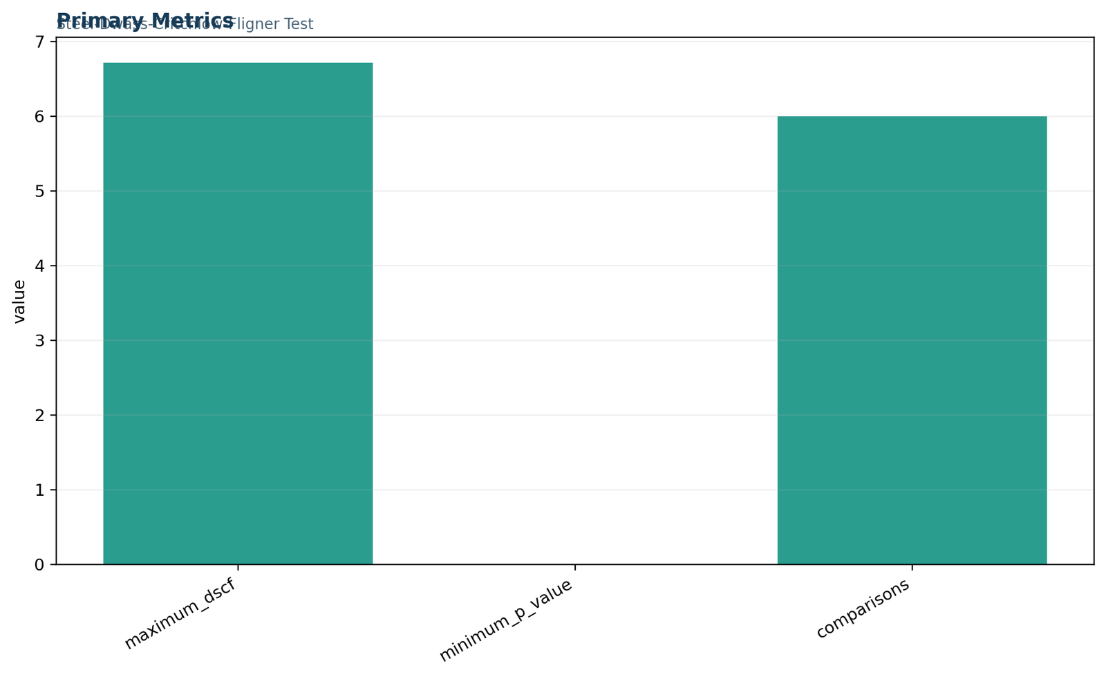
Python chart 1: primary metrics
The full-width summary reports N = 649, four groups, six comparisons, maximum DSCF = 6.717192, and minimum adjusted p = 0.00001211. It provides a rapid audit of the family size and strongest contrast.
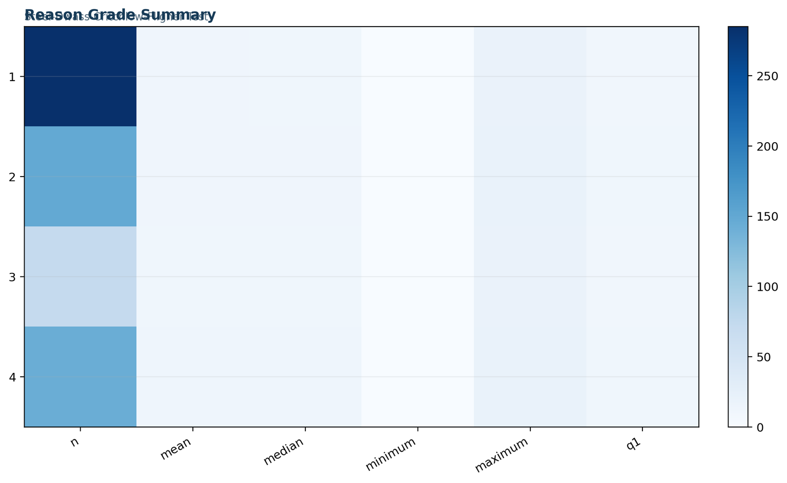
Python chart 2: reason-group grade summary
The descriptive panel compares counts, means, medians, quartiles and ranges. Reputation is highest descriptively, other is lowest by mean and mean rank, and home lies above course. These summaries establish direction for the pairwise results.
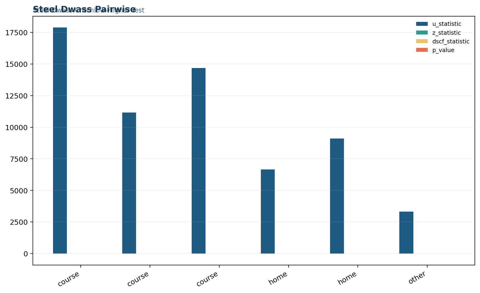
Python chart 3: pairwise DSCF comparisons
The pairwise chart displays all six independently reranked contrasts. Course–reputation produces the maximum DSCF statistic, while course–other produces the weakest evidence. The chart should be read with the exact table because small probabilities require scientific notation.
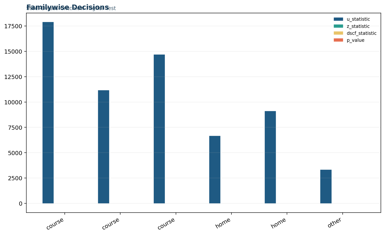
Python chart 4: familywise decisions
Four comparisons cross the .05 familywise threshold and two do not. This chart communicates the decision pattern without implying that nonsignificant pairs have proven identical.
The supplied Python set contains four charts rather than five. The layout therefore uses a full-width primary summary, a paired middle row, and a full-width decision chart. No unsupplied Python image is invented. Every source image is 1600 pixels wide and remains readable in the approved responsive layout.
Steel Dwass Test in R: PMCMRplus workflow and charts
R provides a dedicated all-pairs implementation through PMCMRplus.
The Steel Dwass Test in R can be run with dscfAllPairsTest(). The formula interface accepts a numeric response and independent grouping factor. The result should be checked against group order, pair labels, and the six probabilities in the verified workbook.
library(PMCMRplus)df <- read.csv("student_grades.csv")
df$reason <- factor(df$reason)
# Optional omnibus description.
kruskal.test(G3 ~ reason, data = df)
# Dwass-Steele-Critchlow-Fligner all-pairs procedure.
fit <- dscfAllPairsTest(G3 ~ reason, data = df)
print(fit)
# Each pair is pooled and reranked independently. The reported probabilities
# already use the studentized-range familywise reference distribution.
R documentation describes the method as the Dwass–Steel–Critchlow–Fligner all-pairs test. Each pair is ranked separately. This is the key difference from procedures that reuse one global rank vector. The result matrix should reproduce p = .03378, .659224, .00001211, .0174009, .132591 and .0001134 for the six pairs in the stated order.
R chart 1: primary metrics
The R section begins with the same full-width pattern as Python. Maximum DSCF is 6.717192, the minimum familywise p-value is 0.00001211, and the comparison family contains six pairs.
R chart 2: reason-group grade summary
The group summary supports interpretation of signed pairwise statistics. Median grades are 11, 12, 11 and 13 for course, home, other and reputation, respectively.
R chart 3: DSCF pairwise comparisons
All six contrasts are shown on the same familywise scale. The figure reinforces that course–reputation and other–reputation provide the strongest evidence.
R chart 4: familywise decisions
The decision panel identifies four rejected pairwise nulls and two retained nulls using the already-adjusted .05 criterion.
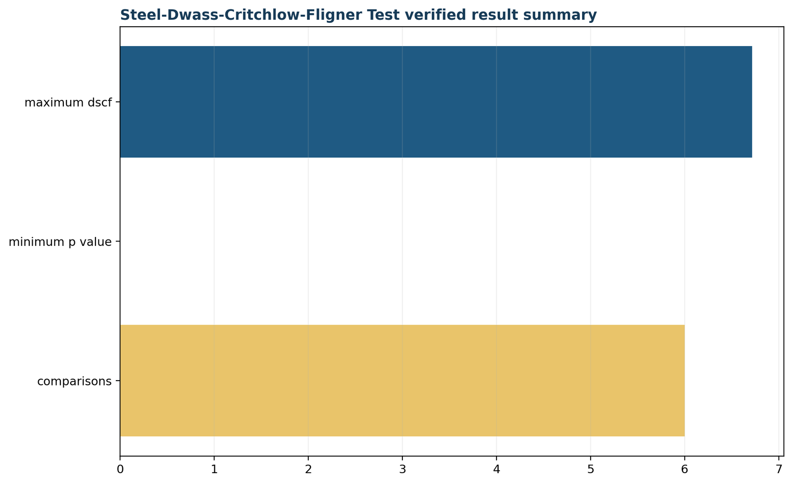
R chart 5: verified result summary
The final R chart verifies the maximum statistic, minimum probability and total number of comparisons. It serves as a compact reproducibility endpoint for the complete analysis.
The R and Python layouts use the same visual rule: chart 1 is full width, charts 2 and 3 share the next row, and remaining supplied charts occupy the next available grid positions. Because R has one additional verified-summary chart, charts 4 and 5 form a balanced final row. On mobile, every chart collapses to one column.
Steel Dwass Test SPSS workflow and limitations
SPSS supplies the omnibus analysis and data checks, but a true DSCF procedure requires custom or integrated computation.
A Steel Dwass Test SPSS analysis must distinguish the native Kruskal–Wallis workflow from the DSCF all-pairs calculation. SPSS can provide the omnibus H statistic, descriptives, quartiles and global mean ranks. Its standard pairwise output should not automatically be relabeled as DSCF because the ranking scope and multiplicity method can differ.
* Native SPSS produces the Kruskal-Wallis omnibus result and can create

* descriptive tables and overall ranks.

NPAR TESTS

/K-W=G3 BY reason_n(1 4)

/STATISTICS=DESCRIPTIVES QUARTILES.* A true DSCF analysis requires custom pairwise reranking and studentized-range

* probabilities. Do not label SPSS's default Dunn-style pairwise table as

* Steel-Dwass-Critchlow-Fligner. Use validated Python/R integration, custom

* syntax, or the supplied audited workbook for the DSCF calculations.
What the supplied SPSS report verifies
The report confirms 649 valid cases, group mean ranks of 296.42, 345.73, 269.17 and 388.48, and Kruskal–Wallis H = 31.625 with df = 3 and p < .001. It then appends the independently verified DSCF summary: six comparisons, maximum statistic 6.717192, minimum p 0.00001211, and cross-check status pass.
This separation is honest. It uses SPSS for its native strengths without pretending that a custom DSCF computation came from a standard menu table.
Recommended quality-control sequence
Steel Dwass Test Excel calculation and workbook audit
The supplied workbook reconstructs every pair and verifies the studentized-range results.
The Steel Dwass Test Excel workbook separates raw inputs, pair-specific ranks, tie contributions, test statistics, diagnostics and reporting. This structure makes the analysis auditable even though standard Excel does not provide a native studentized-range probability function.
For every group pair, create a separate pooled block.1. Pair-specific midrank:
=RANK.AVG(value,pair_value_range,1)
2. Wilcoxon U for group 1:
U = rank_sum_1 - n1*(n1+1)/2
3. Tie-corrected variance:
V = n1*n2/12 * ((Npair+1) - SUM(t^3-t)/(Npair*(Npair-1)))
4. Signed standardized statistic:
z = (U - n1*n2/2)/SQRT(V)
5. DSCF statistic:
q = SQRT(2)*ABS(z)
6. Familywise p-value:
Use the upper tail of the studentized-range distribution with k groups and
infinite degrees of freedom. Standard Excel has no direct studentized-range
function, so the workbook stores independently verified probabilities and
cross-checks every U, variance, z, and q value.
| Workbook sheet | Purpose | Key quality check |
|---|---|---|
| Guide | Documents design, variables, formula and alpha. | Correct method identity. |
| Data_Input | Stores the unchanged G3 and reason values. | 649 source rows. |
| Working | Creates six isolated pairs, midranks and tie contributions. | Ranks are recomputed inside every pair. |
| Calculations | Summarizes maximum DSCF and minimum p. | Maximum = 6.717192. |
| Diagnostics | Documents ranking scope and multiplicity. | One studentized-range family. |
| Reporting | Compares workbook and verified references. | Absolute differences equal zero. |
The workbook’s most important safeguard is not formatting; it is row-level lineage. A reviewer can trace each raw grade into a specific pair, inspect its pair-specific midrank and verify the tie block. That makes the spreadsheet substantially more reliable than a calculator that displays only six p-values.
Steel Dwass Test in MATLAB and SAS
SAS offers a native DSCF option; MATLAB generally requires a custom implementation.
SAS
proc npar1way data=student dscf;

class reason;

var G3;

run;/* The DSCF option requests pairwise two-sample rankings and displays

familywise-adjusted Steel-Dwass-Critchlow-Fligner comparisons. */
The DSCF option in PROC NPAR1WAY is a direct implementation based on pairwise two-sample rankings. Report the pair labels, DSCF statistics and adjusted probabilities shown by the procedure. Confirm the class ordering before assigning direction.
MATLAB
% MATLAB has no standard built-in Steel-Dwass command.

% For each pair: pool the two samples, assign tied midranks, compute the

% tie-corrected Wilcoxon z statistic, and set q = sqrt(2)*abs(z).

% Evaluate q with a validated studentized-range survival function using the

% total number of groups. Cross-check against R, Python, SAS, or the workbook.
A custom MATLAB workflow must reproduce pair-specific ties and the studentized-range survival probability. Validate all six outputs against a documented implementation rather than relying on a collection of unadjusted ranksum tests.
Software agreement should be numeric, not merely verbal. A correct implementation will reproduce the six DSCF statistics to reasonable floating-point precision and the same familywise decisions. Small formatting differences are acceptable; different pairwise rankings or a second multiplicity adjustment are not.
Steel Dwass vs Dunn, Conover, Nemenyi and Mann–Whitney tests
The post-hoc method should match the ranking scope and inferential family.
Comparing the Steel Dwass Test with Dunn, Conover and Nemenyi procedures clarifies why post-hoc results can differ. These tests do not merely apply different labels to the same calculation; they use different statistics, ranking schemes and multiplicity references.
| Method | Ranking scope | Multiplicity | Typical use | Main distinction |
|---|---|---|---|---|
| Steel–Dwass / DSCF | Rerank inside every pair | Studentized range | All pairs among independent groups | Pair-specific Wilcoxon structure |
| Dunn’s test | Global omnibus ranks | Bonferroni, Holm or related adjustment | Post-hoc comparisons after Kruskal–Wallis | Reuses complete-sample ranks |
| Conover test | Global ranks | Adjusted pairwise probabilities | Powerful rank post-hoc procedure | Different variance construction |
| Nemenyi test | Mean ranks | Studentized range | All-pairs comparisons | Often described through critical rank differences |
| Mann–Whitney U | One pair only | None unless added | Single prespecified two-group comparison | Does not by itself control an all-pairs family |
The DSCF method is often attractive because every contrast behaves like a carefully standardized two-sample rank test while the family is handled simultaneously. Dunn’s method is often more familiar and widely implemented. Conover can be powerful. Nemenyi has a simple critical-difference interpretation. No method is universally best; the analysis plan should name the chosen procedure before pairwise results are inspected.
For only two groups, an all-pairs procedure is unnecessary. Use a dedicated two-sample method such as Mann–Whitney U, Brunner–Munzel or the two-sample Kolmogorov–Smirnov test, depending on the estimand.
Practical Steel Dwass Test interpretation and verification guide
The Steel Dwass Test should be interpreted as a coordinated family of rank comparisons rather than a collection of unrelated p-values. For each pair, the Steel Dwass Test asks whether the pooled rank behavior is more separated than expected under equality of the two distributions, while the studentized-range reference protects the entire comparison family. This means that course versus home cannot be interpreted independently of the fact that five other comparisons were also evaluated. The Steel Dwass Test makes that multiplicity visible in the calculation itself. Analysts who understand this structure are less likely to apply an unnecessary second correction or to report only the pairs that happen to be significant.
A good Steel Dwass Test audit begins before any p-value is examined. Verify the group labels, sample sizes, missing-data rule, direction of the outcome scale and scientific meaning of the family. Then confirm that the Steel Dwass Test implementation isolates each pair and recalculates average ranks and tie corrections inside that pair. The pair-specific U statistic should agree with an independently calculated Mann–Whitney U statistic for the same two groups, but the final probability must come from the familywise DSCF distribution. This distinction separates the Steel Dwass Test from a sequence of unadjusted two-sample tests.
The Steel Dwass Test also requires careful direction reporting. The displayed DSCF statistic is nonnegative because it uses the absolute standardized Wilcoxon statistic. Direction therefore comes from the signed z value and the group summaries. In the present Steel Dwass Test, negative z values for course–home, course–reputation and other–reputation align with lower grades in the first-listed group. The positive home–other z aligns with higher grades in home. The Steel Dwass Test result table should always preserve the pair order so that these signs remain meaningful. Readers can review descriptive statistics, mean, median and mode, and frequency distributions when checking direction.
Another practical issue is the relationship between the Steel Dwass Test and the omnibus analysis. The significant Kruskal–Wallis statistic establishes that at least one distributional contrast exists, but it does not determine which pair is different. The Steel Dwass Test resolves that ambiguity through six simultaneous comparisons. Still, the Steel Dwass Test should not be described as automatically valid only because the omnibus p-value is small. Independence, appropriate grouping, rankable outcomes and a prespecified family remain essential. The broader logic of hypothesis testing, the null and alternative hypothesis, and p-value interpretation applies to each pair.
For tied grades, the Steel Dwass Test needs more than average ranks. The null variance must reflect the tied blocks within the particular pair. A tie pattern found in course versus home is not necessarily the same tie pattern found in course versus reputation, so the Steel Dwass Test recalculates the variance six times. This is why the workbook stores t³ − t contributions in the pairwise working sheet. A dependable Steel Dwass Test calculator should expose or document that correction. General background on variance, standard deviation, standard error and the interquartile range helps readers separate descriptive spread from the tie-adjusted rank variance used in the test.
The Steel Dwass Test is robust to many features that make ordinary mean comparisons uncomfortable, but robust does not mean immune to study-design problems. Dependence, uncontrolled clustering, poorly defined categories or selective deletion can invalidate the Steel Dwass Test just as they can invalidate parametric procedures. Extreme values should be inspected through outlier detection, box-plot interpretation and histogram interpretation. The Steel Dwass Test converts magnitudes into ranks, but an extreme observation can still influence ordering and tied-block structure. Transparent diagnostics make the Steel Dwass Test result easier to defend.
Power and practical importance should be discussed separately from significance. A Steel Dwass Test probability answers whether the pairwise evidence is strong under the familywise reference, not whether the observed difference is educationally important. The Steel Dwass Test does not provide a universal effect-size estimate or confidence interval for every pair. Analysts may add a probability-of-superiority measure, rank-biserial effect or a carefully chosen location estimate when those quantities match the research question. Guidance on effect size, statistical power, confidence intervals and margin of error can support that second layer of interpretation.
Finally, software outputs should be reconciled numerically. The Python Steel Dwass Test p-value matrix, the R Steel Dwass Test result, the SAS DSCF table and the audited Excel workbook should identify the same pairs and produce the same decisions. SPSS can provide the omnibus and descriptive context, but a custom Steel Dwass Test calculation must be labeled clearly. Readers who work across software can consult analysis in Python, analysis in R, analysis in SPSS and Excel analysis workflows. Agreement across platforms is one of the strongest quality checks for the Steel Dwass Test.
Steel Dwass Test diagnostics, sensitivity checks and common errors
Strong reporting verifies the family, the ranks, the ties and the direction of every significant result.
Diagnostic checklist
Common errors
The most serious error is reusing omnibus ranks while labeling the result Steel–Dwass. Another is applying Bonferroni to DSCF-adjusted p-values. Other mistakes include reporting only significant pairs, interpreting the unsigned DSCF statistic as directional, ignoring group labels in a matrix, or claiming that a nonsignificant pair is equivalent.
A final common error is treating the method as a test of means. Rank procedures target distributional ordering. Means can help describe direction, but they are not the tested statistic.
Small groups deserve special attention. The other group has n = 72, much smaller than course at n = 285. Its standard deviation is also the largest at 3.931. Pair-specific ranking handles unequal n, but precision remains sample-dependent. Report sample sizes beside p-values and avoid interpreting a nonsignificant result as absence of a practically important difference.
Effect size should not be improvised from DSCF alone. Supplement pairwise p-values with an estimand such as a probability of superiority, rank-biserial correlation or Hodges–Lehmann difference when appropriate. Review effect size and confidence interval guidance. The supplied analysis focuses on the verified hypothesis tests because those are the quantities supported by the workbook.
How to report the Steel Dwass Test in APA style
Report the omnibus context, method name, pair-specific adjusted probabilities and substantive directions.
APA-style results paragraph
“Final grades differed across school-choice reason groups, Kruskal–Wallis H(3) = 31.62, p < .001. Dwass–Steel–Critchlow–Fligner all-pairs comparisons, based on separate pooled rankings for each pair and studentized-range familywise probabilities, identified significant differences between course and home (DSCF = 3.84, p = .034), course and reputation (DSCF = 6.72, p < .001), home and other (DSCF = 4.15, p = .017), and other and reputation (DSCF = 6.04, p < .001). Course versus other (p = .659) and home versus reputation (p = .133) were not significant. Descriptive medians were 11, 12, 11 and 13 for course, home, other and reputation, respectively.”
For very small probabilities, report p < .001 in prose and retain the exact scientific-notation value in a table or supplement. Do not write p = .000. Include the multiplicity method so readers know that the six p-values are already adjusted.
Report direction through descriptive statistics or the signed z statistic. Because DSCF = √2|z|, DSCF itself has no sign. A sentence such as “reputation grades tended higher than course grades” is supported by medians, means and ranks; a sentence such as “positive DSCF shows reputation is higher” is not.
Steel Dwass Test downloads and reproducibility files
Use the supplied reports and workbook to audit every result.
Official implementation sources and verification notes
The method and software guidance were checked against primary documentation.
Python documentation
The scikit-posthocs documentation defines posthoc_dscf as the Dwass–Steel–Critchlow–Fligner all-pairs comparison for a one-factor independent-groups layout. Its interface accepts either an array or a data frame with value and group columns.
R documentation
CRAN documentation for PMCMRplus identifies dscfAllPairsTest() as the all-pairs procedure according to Dwass, Steel, Critchlow and Fligner. This supports the formula-interface workflow shown above.
SAS documentation
Official PROC NPAR1WAY documentation states that the DSCF option computes multiple comparisons based on pairwise two-sample Wilcoxon rankings. This confirms pair-specific rather than omnibus ranking.
The uploaded workbook independently reproduces the pair statistics and matches the verified references with zero absolute difference for the maximum DSCF statistic, comparison count and minimum p-value. The Python PDF supplies the complete six-row pairwise table. The SPSS report confirms the omnibus result and clearly separates native output from the custom DSCF summary.
Steel Dwass Test frequently asked questions
Concise answers to common questions about formula, interpretation, software and multiplicity.
What is the Steel Dwass Test?
It is a nonparametric all-pairs multiple-comparison procedure for independent groups. Each pair is pooled and reranked separately, then evaluated with a studentized-range familywise adjustment.
Is Steel–Dwass the same as DSCF?
In practice, Steel–Dwass commonly refers to the Dwass–Steel–Critchlow–Fligner procedure. State the full name once because naming order varies across software and publications.
Must Kruskal–Wallis be significant first?
A significant omnibus test is a common post-hoc context, but the DSCF familywise procedure can directly test a prespecified family of pairs. The analysis plan should define whether the omnibus test is descriptive context or a formal gatekeeper.
Why are ranks recomputed for every pair?
Pair-specific reranking makes each comparison a true standardized two-sample Wilcoxon contrast. It is the defining computational distinction from global-rank methods such as Dunn’s procedure.
Are Steel Dwass p-values already adjusted?
Yes. The probabilities come from a studentized-range familywise distribution. Do not apply another Bonferroni or Holm correction unless you are deliberately redefining a larger inferential family.
How are ties handled?
Tied values receive average ranks within each pair, and the variance includes a tie correction based on the sizes of the tied blocks.
What does a negative z mean?
Under the listed group order, a negative signed Wilcoxon z generally indicates that the first group tends to have lower ranks. Always verify direction with medians, means or mean ranks because software ordering can differ.
Why is the DSCF statistic always positive?
The statistic is √2 times the absolute pairwise z. Its magnitude determines significance; direction is retained separately in the signed z and descriptive summaries.
Can SPSS run the procedure natively?
SPSS can run Kruskal–Wallis and native pairwise procedures, but a true DSCF calculation generally requires custom syntax, integrated Python or R, or an external verified implementation. Do not relabel a default Dunn-style table.
Which pairs were significant in this example?
Course–home, course–reputation, home–other and other–reputation were significant. Course–other and home–reputation were not significant at familywise α = .05.
Does a nonsignificant pair prove equality?
No. It indicates insufficient evidence for a difference under the selected familywise test. Equivalence requires a prespecified negligible-effect region and a dedicated equivalence design.
What should an online calculator display?
It should display group labels and sizes, pair-specific U or rank sums, tie-corrected z, DSCF, familywise p-values, the number of groups, alpha, and a clear statement that probabilities are already adjusted.