
.bmt-post,.bmt-post *{box-sizing:border-box}
.bmt-post{–ink:#10243e;–muted:#52657c;–line:#d8e3ef;–soft:#f4f8fc;–blue:#0b5fa5;–navy:#07345c;–cyan:#eaf6ff;–green:#0b7a5a;–green-soft:#eaf8f3;–gold:#ad6d00;–gold-soft:#fff7e5;–red:#a42a2a;–red-soft:#fff0f0;–shadow:0 18px 50px rgba(13,52,86,.10);font-family:Inter,system-ui,-apple-system,BlinkMacSystemFont,”Segoe UI”,Roboto,Arial,sans-serif;color:var(–ink);line-height:1.72;background:#fff;width:min(1480px,calc(100vw – 32px))!important;max-width:1480px!important;margin:24px 0 48px 50%!important;transform:translateX(-50%)!important;border:1px solid var(–line);border-radius:24px;box-shadow:var(–shadow);overflow:hidden;position:relative}
.bmt-post a{color:#075fa5;text-decoration-thickness:1px;text-underline-offset:3px}.bmt-post a:hover{color:#033b68}.bmt-shell{padding:clamp(20px,3.2vw,54px)}
.bmt-hero{padding:clamp(34px,5vw,72px);background:linear-gradient(135deg,#062f55 0%,#0a5b98 58%,#1680b8 100%);color:#fff;position:relative;overflow:hidden}.bmt-hero:after{content:””;position:absolute;width:440px;height:440px;border-radius:50%;right:-190px;top:-220px;background:rgba(255,255,255,.10)}
.bmt-kicker{display:inline-flex;align-items:center;gap:9px;padding:8px 13px;border-radius:999px;background:rgba(255,255,255,.14);border:1px solid rgba(255,255,255,.25);font-size:.82rem;font-weight:800;letter-spacing:.08em;text-transform:uppercase}.bmt-hero h1{color:#fff!important;font-size:clamp(2rem,4.5vw,4.25rem)!important;line-height:1.08!important;margin:20px 0 18px!important;max-width:1120px}.bmt-hero p{font-size:clamp(1.05rem,1.5vw,1.28rem);max-width:1080px;margin:0;color:#eaf5ff}.bmt-badges{display:flex;flex-wrap:wrap;gap:9px;margin-top:24px}.bmt-badge{padding:8px 12px;border-radius:999px;background:#fff;color:#07345c;font-weight:800;font-size:.86rem}
.bmt-ad{margin:0;padding:18px;text-align:center;border-top:1px solid var(–line);border-bottom:1px solid var(–line);background:#fbfdff;color:#708198;font-size:.76rem;letter-spacing:.12em;text-transform:uppercase}
.bmt-post h2{font-size:clamp(1.55rem,2.5vw,2.35rem)!important;line-height:1.2!important;margin:0 0 18px!important;color:#082d50!important}.bmt-post h3{font-size:clamp(1.18rem,1.65vw,1.48rem)!important;line-height:1.3!important;margin:0 0 10px!important;color:#10395d!important}.bmt-post p{margin:0 0 16px}.bmt-post section{scroll-margin-top:90px}.bmt-section{padding:clamp(28px,4vw,56px);border-top:1px solid var(–line)}.bmt-lead{font-size:1.08rem;color:#304b67}.bmt-note{padding:18px 20px;border-left:5px solid var(–blue);background:var(–cyan);border-radius:0 14px 14px 0;margin:18px 0}.bmt-good{border-left-color:var(–green);background:var(–green-soft)}.bmt-warn{border-left-color:var(–gold);background:var(–gold-soft)}.bmt-danger{border-left-color:var(–red);background:var(–red-soft)}
.bmt-grid{display:grid;grid-template-columns:repeat(2,minmax(0,1fr));gap:20px}.bmt-grid-3{display:grid;grid-template-columns:repeat(3,minmax(0,1fr));gap:18px}.bmt-card{border:1px solid var(–line);border-radius:18px;padding:22px;background:#fff;min-width:0}.bmt-card.soft{background:var(–soft)}.bmt-card h3{margin-top:0!important}.bmt-metric{display:flex;flex-direction:column;justify-content:center;min-height:145px}.bmt-metric strong{font-size:clamp(1.65rem,3vw,2.5rem);line-height:1.1;color:#073b68}.bmt-metric span{color:var(–muted);font-weight:700;margin-top:8px}.bmt-metric small{color:#6a7b8e;margin-top:7px}
.bmt-toc{background:#f6fafe;border:1px solid var(–line);border-radius:18px;padding:22px}.bmt-toc ol{columns:2;column-gap:38px;margin:0;padding-left:22px}.bmt-toc li{break-inside:avoid;margin:7px 0}.bmt-toc a{text-decoration:none;font-weight:700}
.bmt-table-wrap{width:100%;overflow-x:auto;-webkit-overflow-scrolling:touch;border:1px solid var(–line);border-radius:16px;margin:18px 0}.bmt-table{width:100%;min-width:760px;border-collapse:collapse;background:#fff}.bmt-table th,.bmt-table td{padding:13px 15px;text-align:left;vertical-align:top;border-bottom:1px solid var(–line)}.bmt-table th{background:#0a4e83;color:#fff;font-size:.9rem}.bmt-table tr:last-child td{border-bottom:0}.bmt-table tbody tr:nth-child(even){background:#f8fbfe}.bmt-table.compact{min-width:660px}
.bmt-formula{font-family:Georgia,”Times New Roman”,serif;font-size:clamp(1.06rem,1.7vw,1.35rem);line-height:1.75;padding:18px 20px;background:#f7fbff;border:1px solid #cbddec;border-radius:14px;overflow-wrap:anywhere;margin:14px 0}.bmt-formula b{font-family:Inter,system-ui,sans-serif;color:#073b68}.bmt-steps{counter-reset:bmt-step;display:grid;gap:14px}.bmt-step{counter-increment:bmt-step;display:grid;grid-template-columns:48px minmax(0,1fr);gap:15px;align-items:start;padding:18px;border:1px solid var(–line);border-radius:16px;background:#fff}.bmt-step:before{content:counter(bmt-step);display:grid;place-items:center;width:42px;height:42px;border-radius:13px;background:#083e6c;color:#fff;font-weight:900}
.bmt-code{position:relative;margin:16px 0}.bmt-code-label{display:inline-block;padding:7px 11px;background:#0d365a;color:#fff;border-radius:10px 10px 0 0;font-size:.78rem;font-weight:800;letter-spacing:.05em;text-transform:uppercase}.bmt-code pre{margin:0!important;background:#071c2f!important;color:#e8f4ff!important;padding:20px!important;border-radius:0 14px 14px 14px!important;overflow:auto!important;white-space:pre!important;font-size:.88rem!important;line-height:1.65!important;max-width:100%!important}.bmt-code code{font-family:Consolas,Monaco,”Courier New”,monospace!important}
.bmt-chart{margin:22px 0;border:1px solid var(–line);border-radius:19px;overflow:hidden;background:#fff}.bmt-chart img{display:block;width:100%!important;height:auto!important;max-width:100%!important}.bmt-chart-body{padding:20px}.bmt-chart-body h3{margin-bottom:8px!important}.bmt-caption{color:#5b6f84;font-size:.92rem}.bmt-chart-grid{display:grid;grid-template-columns:repeat(2,minmax(0,1fr));gap:20px}.bmt-chart-grid .bmt-chart{margin:0}
.bmt-downloads{display:grid;grid-template-columns:repeat(4,minmax(0,1fr));gap:14px}.bmt-download{display:flex;flex-direction:column;gap:5px;padding:18px;border-radius:15px;background:#073b68;color:#fff!important;text-decoration:none!important;min-height:116px;justify-content:center}.bmt-download:hover{background:#0a568f;color:#fff!important}.bmt-download strong{font-size:1rem}.bmt-download span{color:#d8ecff;font-size:.86rem}
.bmt-check{list-style:none;padding:0;margin:10px 0}.bmt-check li{position:relative;padding:7px 0 7px 30px}.bmt-check li:before{content:”✓”;position:absolute;left:0;top:6px;width:21px;height:21px;border-radius:50%;display:grid;place-items:center;background:#dff5ec;color:#087251;font-weight:900}.bmt-cross li:before{content:”×”;background:#ffe9e9;color:#9b2424}
.bmt-report{padding:22px;border:2px solid #bcd2e6;border-radius:16px;background:#fbfdff;font-family:Georgia,”Times New Roman”,serif;font-size:1.05rem}.bmt-faq details{border:1px solid var(–line);border-radius:14px;padding:0 17px;background:#fff;margin:11px 0}.bmt-faq summary{cursor:pointer;font-weight:850;padding:17px 30px 17px 0;color:#0b365b}.bmt-faq details p{padding:0 0 17px;margin:0;color:#3f566d}.bmt-footer{padding:32px clamp(24px,4vw,56px);background:#062f55;color:#e9f5ff}.bmt-footer h2{color:#fff!important}.bmt-footer a{color:#fff}.bmt-back{display:inline-block;margin-top:12px;padding:10px 14px;border-radius:10px;background:#fff;color:#07345c!important;text-decoration:none!important;font-weight:800}
@media(max-width:1000px){.bmt-grid-3{grid-template-columns:1fr 1fr}.bmt-downloads{grid-template-columns:1fr 1fr}.bmt-chart-grid{grid-template-columns:1fr}.bmt-toc ol{columns:1}}
@media(max-width:782px){.bmt-post{width:100%!important;max-width:100%!important;margin:0!important;transform:none!important;border-left:0;border-right:0;border-radius:0;box-shadow:none}.bmt-hero,.bmt-section{padding:24px 18px}.bmt-shell{padding:18px}.bmt-grid,.bmt-grid-3,.bmt-downloads{grid-template-columns:1fr}.bmt-card{padding:18px}.bmt-step{grid-template-columns:40px minmax(0,1fr);padding:15px}.bmt-step:before{width:36px;height:36px}.bmt-table{min-width:680px}.bmt-hero h1{font-size:2.18rem!important}.bmt-code pre{font-size:.8rem!important;padding:16px!important}}
Brunner Munzel Test: Formula, Interpretation, R, Python, SPSS, SAS and Excel Guide
The Brunner Munzel test answers a precise question that ordinary median comparisons and the Mann-Whitney U test often do not answer safely: when one observation is selected from each independent population, is either population more likely to produce the larger value? This worked guide calculates the statistic from 649 student records and explains every result, chart and software output.
Brunner Munzel Test Quick Answer
For the worked analysis, the Brunner Munzel test compares final grade G3 between female students (F, n = 383) and male students (M, n = 266). The groups are independent, G3 is ordered numeric data, the sample sizes are unequal, and identical distribution shapes are not assumed.
Brunner Munzel Test Contents
- Definition and research question
- When to use the test
- Null and alternative hypotheses
- Assumptions
- Formula and rank calculation
- Variables and data dictionary
- Worked result
- Chart-by-chart findings
- Brunner Munzel test in Python
- Brunner Munzel test in R
- Brunner Munzel test in SPSS
- Brunner Munzel test in Excel
- Brunner Munzel test in SAS
- Comparison with other tests
- APA reporting
- Downloads
- Frequently asked questions
What Is the Brunner Munzel Test?
The Brunner Munzel test is a rank-based nonparametric procedure for comparing two independent populations without requiring equal variances or identically shaped distributions. It was developed for the nonparametric Behrens-Fisher problem: the same broad situation handled by Welch’s t test for means, but expressed through a probability-based relative effect rather than a difference in population means.
The central estimand is p = P(X < Y) + 0.5P(X = Y). It describes the probability that a randomly selected observation from population X is smaller than a randomly selected observation from population Y, with ties split equally. Under stochastic equality, p = 0.5. A value below 0.5 favors larger observations in X; a value above 0.5 favors larger observations in Y. Because the direction depends on group order, every Brunner Munzel test report should name X and Y explicitly.
The method is sometimes called the generalized Wilcoxon test. That name can be useful, but it should not obscure the difference: the Brunner Munzel test studentizes the relative-effect estimator with group-specific rank variability. This is why it remains appropriate when the populations have unequal spreads and different shapes, conditions that complicate the usual interpretation of the Wilcoxon-Mann-Whitney procedure.
When Should You Use the Brunner Munzel Test?
Use the Brunner Munzel test when
- There are exactly two independent groups.
- The response is at least ordinal, so observations can be ranked.
- Normality is doubtful, outliers are influential, or the response is ordinal.
- Unequal variances or different distribution shapes are plausible.
- The research question concerns probabilistic ordering rather than a mean difference.
- You want a robust alternative to a default Mann-Whitney analysis.
Do not use the Brunner Munzel test when
- The same participants are measured twice; use a paired method.
- There are more than two groups without a planned two-group contrast.
- The outcome is purely nominal and cannot be ordered.
- Observations are clustered and the dependence is ignored.
- Your estimand is specifically the arithmetic mean difference.
- Group assignment or sampling makes independence implausible.
The Brunner Munzel test is especially attractive when a box plot or ECDF shows unequal spread. However, test selection should follow the research estimand and design, not a preliminary significance test for equal variances. Read the site’s guide to parametric versus nonparametric tests and the overview of the independent-samples t test before treating any rank test as an automatic fallback.
Brunner Munzel Test Null and Alternative Hypotheses
Write the hypotheses in terms of the relative effect, not generic scale parameters and not an unsupported statement about medians. For the worked Brunner Munzel test, define X as female G3 and Y as male G3.
Two-sided hypothesis used here
H1: p ≠ 0.50
Under H0, neither group is more likely to yield the larger G3 score after ties are divided equally. The two-sided Brunner Munzel test asks whether the relative effect departs in either direction.
Directional alternatives
M tends larger: p > 0.50
Choose a one-sided direction before examining results. Software labels such as less and greater can refer to the first sample, its average rank, or the package’s internal statistic; verify direction with a simple ordered example.
In the observed data, p = 0.421696. Equivalently, P(F > M) + 0.5P(F = M) = 1 – 0.421696 = 0.578304. The Brunner Munzel test therefore estimates a 57.83% tie-adjusted probability that a randomly selected female student has the higher G3 score.
Brunner Munzel Test Assumptions
The Brunner Munzel test is flexible, but it is not assumption-free. The important assumptions concern design and measurement, not normality or equal variances.
1. Independent observations
Each student’s record should contribute once, and one student’s G3 should not determine another student’s score. Repeated measures, matched pairs, siblings within families, or students nested in classrooms may violate independence.
2. Two independent groups
Every usable observation belongs to F or M, not both. The Brunner Munzel test is not the correct procedure for before-after scores from the same students.
3. Ordered response
G3 is numeric and ordered. The method also supports ordinal responses because it uses order and ties rather than requiring interval-scale distances.
4. Representative sampling
Inference beyond the dataset depends on how the records were obtained. A very small p-value cannot repair selection bias or limited population coverage.
5. Usable rank variation
Both groups need enough variation to estimate the group-specific rank variances. Degenerate samples can produce undefined statistics or software warnings.
6. Prespecified analysis
Choose groups, outcome, alternative and handling of missing values before inspecting the result. This protects the Brunner Munzel test from outcome-driven decisions.
Brunner Munzel Test Formula and Calculation
The Brunner Munzel test begins with pooled midranks and within-group midranks. Let n1 and n2 be the two group sizes. For observation j in group i, let Rij be its midrank in the pooled sample and R*ij its midrank within its own group.
p̂ = P̂(X < Y) + 0.5P̂(X = Y) = [number of X<Y pairs + 0.5(number of tied pairs)] / (n1n2)
D1j = R1j – R*1j, D2j = R2j – R*2j
si2 = Σ(Dij – D̄i)2 / (ni – 1)
W = n1n2(R̄2 – R̄1) / [(n1 + n2)√(n1s12 + n2s22)]
df = (n1s12 + n2s22)2 / {[(n1s12)2/(n1-1)] + [(n2s22)2/(n2-1)]}
The name “nonparametric Behrens-Fisher” becomes clear here: the Brunner Munzel test uses separate rank-variance contributions and a Welch-type degrees-of-freedom approximation. The p-value is commonly obtained from a t distribution. SciPy defaults to the t reference distribution, while a normal option is available for large-sample approximation.
Variables Used in the Brunner Munzel Test
| Role | Variable | Coding | Meaning in this analysis |
|---|---|---|---|
| Outcome | G3 | Numeric final grade, observed 0-19 | The ordered response compared by the Brunner Munzel test. |
| Grouping variable | sex | F or M | Defines two independent samples. F is X/group 1 and M is Y/group 2. |
| Sample X | F | n = 383 | Mean 12.2533, median 12, SD 3.1241, IQR 10-14. |
| Sample Y | M | n = 266 | Mean 11.4060, median 11, SD 3.3207, IQR 10-13. |
| Relative effect | p | 0 to 1 | P(F<M) + 0.5P(F=M); null value 0.50. |
| Decision threshold | α | 0.05 | Prespecified significance level for the two-sided test. |
All 649 records had usable values for the selected variables in the supplied reports. The Brunner Munzel test therefore used 383 F observations and 266 M observations. For more on summaries such as means, quartiles and spread, see descriptive statistics, standard deviation and interquartile range.
Worked Brunner Munzel Test Result
The worked Brunner-Munzel method uses 101,878 cross-group pairs (383 × 266). Of these, 37,750 pairs have F < M, 53,705 have F > M, and 10,423 are tied. Splitting ties equally gives:
The complementary F-superiority effect is 1 – 0.4216956 = 0.5783044. The pooled mean rank is 345.829 for F and 295.009 for M. The rank-variance components are 5,761.750 for F and 11,587.195 for M. Studentization produces W = -3.468824 and df = 575.612839.
| Component | F | M | Interpretation |
|---|---|---|---|
| Sample size | 383 | 266 | Unequal sample sizes are permitted. |
| Mean G3 | 12.2533 | 11.4060 | Descriptive difference = 0.8472 points. |
| Median G3 | 12 | 11 | Descriptive only; the Brunner-Munzel method does not directly test medians. |
| Standard deviation | 3.1241 | 3.3207 | Spreads differ modestly; equal spread is not required. |
| Mean pooled rank | 345.8290 | 295.0094 | Higher pooled ranks for F support larger F scores. |
| W statistic | -3.468824 | Sign reflects the selected group order. | |
| Degrees of freedom | 575.612839 | Welch-type approximation. | |
| Two-sided p-value | 0.000561828 | Reject H0 at α = .05. | |
| Relative effect | 0.421696 | F-favoring complement = 0.578304. | |
Brunner Munzel Test Charts and Statistical Meaning
Visuals do not replace the Brunner-Munzel method. They show why a probability-based rank comparison is informative and help readers detect features that a single p-value cannot communicate.
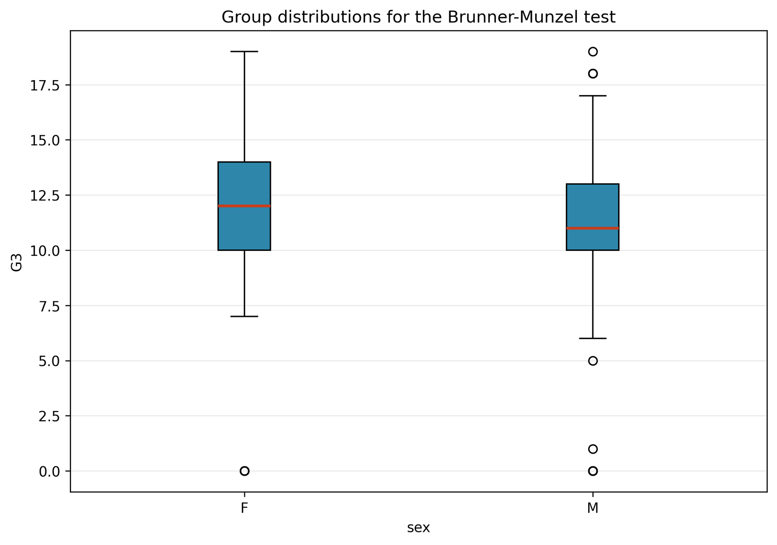
1. Group box plots
Female G3 has median 12 and IQR 10-14; male G3 has median 11 and IQR 10-13. Both groups contain low-score outliers, and the male group includes several extreme observations. The boxes overlap substantially, so the Brunner-Munzel method is identifying a probabilistic tendency, not complete separation.
Next step: report medians and IQRs as descriptive summaries, then report the relative effect as the inferential target.
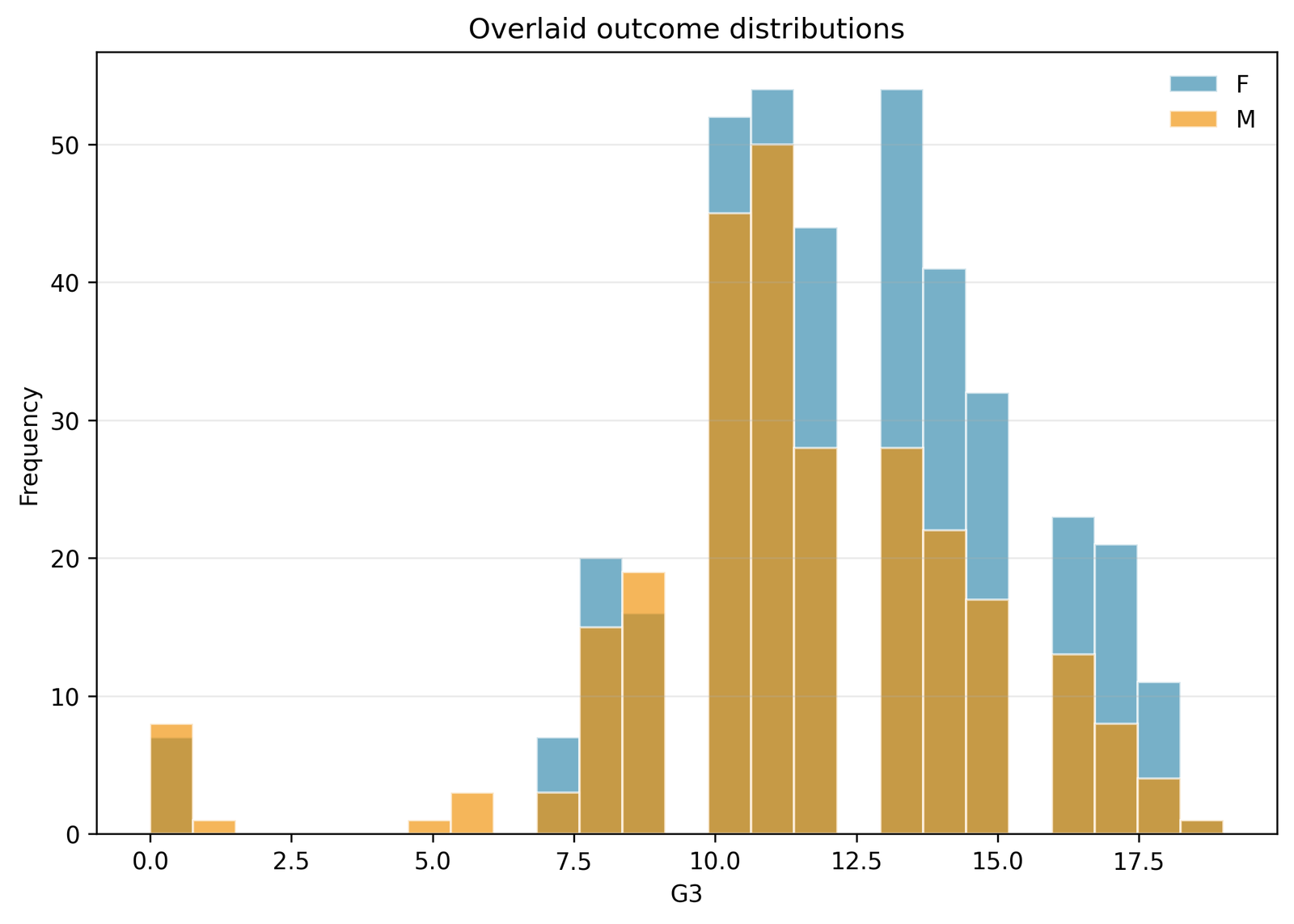
2. Distribution overlay
The discrete G3 scale creates many ties, especially from 10 through 14. Female frequencies are relatively stronger at several higher scores, while male frequencies are more concentrated around lower central values. Ties are not discarded: the Brunner-Munzel method allocates half of every tied pair to each direction.
Next step: avoid describing this chart as proof of normality or as a test of equal variances.
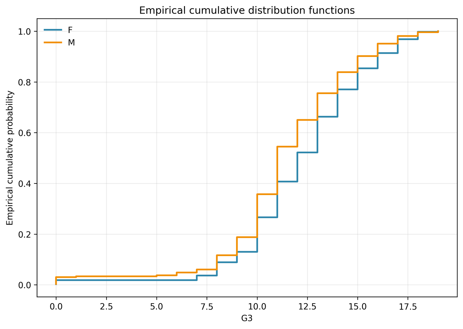
3. Empirical cumulative distributions
Across much of the middle score range, the male ECDF lies above the female ECDF. At a fixed G3 threshold, a higher ECDF means a larger proportion has accumulated at or below that threshold. This pattern is consistent with female scores tending higher, which agrees with the Brunner-Munzel method direction.
Next step: note that crossing ECDFs would make simple location-shift language even less defensible.
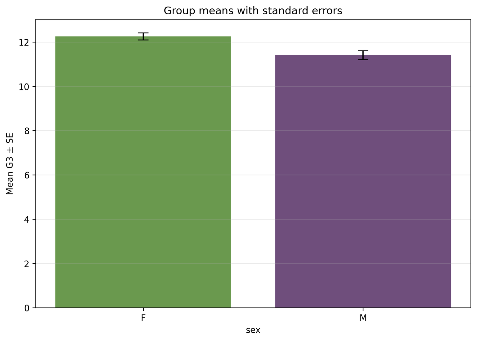
4. Means with standard errors
Mean G3 is 12.2533 for F and 11.4060 for M. The standard errors are approximately 0.1596 and 0.2036. This chart is descriptive because the Brunner-Munzel method targets relative effect, not the arithmetic mean. Include it to describe the data, not to redefine the null hypothesis.
Next step: use Welch’s t test when the scientific estimand is specifically a difference in population means.
Brunner Munzel Test in Python
The most direct Brunner-Munzel method in Python uses scipy.stats.brunnermunzel. SciPy accepts two one-dimensional samples, supports two-sided and one-sided alternatives, and offers t or normal reference distributions. The t distribution is the default and matches the supplied Python and R reports.
import pandas as pd
from scipy import stats

# Read the data and preserve the intended group order.
df = pd.read_csv("dataset.csv")
x = df.loc[df["sex"].eq("F"), "G3"].dropna().to_numpy()
y = df.loc[df["sex"].eq("M"), "G3"].dropna().to_numpy()

result = stats.brunnermunzel(
    x,
    y,
    alternative="two-sided",
    distribution="t"
)

less = sum(a < b for a in x for b in y)
ties = sum(a == b for a in x for b in y)
relative_effect = (less + 0.5 * ties) / (len(x) * len(y))

print(f"W = {result.statistic:.6f}")
print(f"p = {result.pvalue:.9f}")
print(f"P(X<Y)+0.5P(X=Y) = {relative_effect:.6f}")W = -3.468824
p = 0.000561828
P(X<Y)+0.5P(X=Y) = 0.421696For this Brunner-Munzel method, using distribution="normal" produces p = 0.000522741 instead of the t-based p = 0.000561828. Both lead to the same decision, but the report must identify the approximation. Do not switch between them silently. The site’s t test in Python guide provides related guidance on reproducible data preparation and software reporting.
Brunner Munzel Test in R
A reliable Brunner-Munzel method in R can be run with the brunnermunzel package. It returns the statistic, degrees of freedom, p-value, confidence interval and relative-effect estimate. The formula interface is convenient, but factor-level order must be verified because the first and second levels determine effect direction.
library(brunnermunzel)

dat <- read.csv("dataset.csv", stringsAsFactors = FALSE)
dat <- subset(dat, sex %in% c("F", "M") & !is.na(G3))
dat$sex <- factor(dat$sex, levels = c("F", "M"))

fit <- brunnermunzel.test(
  G3 ~ sex,
  data = dat,
  alternative = "two.sided",
  alpha = 0.05,
  perm = FALSE,
  est = "original"
)

fit$statistic
fit$parameter
fit$p.value
fit$estimate
fit$conf.intBrunner-Munzel Test Statistic = -3.468824
df = 575.612839
p-value = 0.0005618282
P(X<Y)+0.5P(X=Y) = 0.4216956For a small-sample Brunner-Munzel method in R, set perm = TRUE when exact enumeration is computationally feasible, or use the package’s permutation function. Enumeration grows combinatorially, so large samples automatically require asymptotic or Monte Carlo strategies. This dataset has 649 observations, making full enumeration infeasible and the t approximation appropriate.
The supplied R report gives a bootstrap 95% interval of approximately [0.3798, 0.4655] for the reported effect. The supplied Python report gives [0.3785, 0.4681]. Small differences are expected when bootstrap seeds or percentile procedures differ. Both intervals lie below 0.50 and support the same directional interpretation of the Brunner-Munzel method.
Brunner Munzel Test in SPSS
Standard SPSS menus do not provide a native one-click Brunner-Munzel method in SPSS. The supplied SPSS workflow uses embedded Python to calculate pooled and within-group ranks, estimate W and df, create a prepared SAV file, and export SPV/PDF output. SPSS’s ordinary Mann-Whitney command is included only as familiar descriptive output; it is not a substitute for the custom Brunner-Munzel calculation.
What the supplied SPSS workflow does correctly
- Detects the two groups F and M.
- Uses all 649 valid G3 observations.
- Computes W = -3.468824 and df = 575.612839.
- Computes the relative effect 0.421696.
- Saves prepared data and exports SPV/PDF output.
Important p-value distinction
The embedded standard-library script displays the normal-approximation p-value, approximately 0.000522741, because it does not call a Student-t CDF. The supplied Python and R reports use the Welch-type t reference and report 0.000561828. A careful Brunner-Munzel method report should use the t result as the primary value and label the SPSS normal value as an approximation.
Researchers who need a GUI may also use a validated jamovi implementation rather than relabeling SPSS’s Mann-Whitney output. For broader SPSS workflow guidance, see t tests in SPSS and SPSS, R and data-visualization results.
Brunner Munzel Test in Excel
A transparent Brunner-Munzel method in Excel is possible, but it requires more than ranking the pooled outcome. A correct workbook must calculate pooled midranks, within-group midranks, group-specific variance components, W, Welch-type df and the t-distribution p-value. A workbook that stops at a rank sum is performing a Mann-Whitney-style calculation, not the complete Brunner-Munzel method.
Prepare the two columns
Place F G3 values in one column and M G3 values in another, or retain a long table with group and outcome. Confirm nF = 383 and nM = 266.
Calculate pooled midranks
Stack both groups, then use average ranks for ties. Modern Excel can use RANK.AVG; older files may need a frequency-based table to avoid repeated formulas.
Calculate within-group midranks
Rank F observations within F and M observations within M. Subtract these ranks from the pooled ranks for the group-specific components.
Estimate rank variances
Compute sample variances of pooled-rank minus within-rank components separately for F and M. Do not pool them as one common variance.
Calculate W and df
Apply the studentized statistic and Welch-Satterthwaite formula shown above. The verified targets are W = -3.468824 and df = 575.612839.
Calculate the p-value
Use =T.DIST.2T(ABS(W_cell),df_cell). The expected two-sided p-value is 0.000561828. Use NORM.S.DIST only when explicitly reporting the normal approximation.
The downloadable workbook supplies a worked Brunner-Munzel method in Excel with the full calculation. For related spreadsheet techniques, consult t tests in Excel, percentiles and quartiles and variance.
Brunner Munzel Test in SAS
The keyword Brunner-Munzel method in SAS often leads to a misleading expectation that a standard SAS procedure has a dedicated option. Standard rank-test procedures do not provide the complete studentized Brunner-Munzel calculation as a simple menu choice. A valid implementation generally requires SAS/IML code, a validated macro, or integration with R or Python.
Preferred SAS workflow
- Sort and validate the two independent samples.
- Calculate pooled and within-group midranks.
- Estimate group-specific rank variances.
- Calculate W and Welch-type df.
- Use the Student-t CDF for the p-value.
- Validate against the Python/R targets in this article.
Validation targets
A correct Brunner-Munzel method in SAS for this dataset should reproduce W = -3.468824, df = 575.612839, p = 0.000561828 and p̂ = 0.421696, subject only to sign reversal if group order is reversed.
Do not report PROC NPAR1WAY’s Wilcoxon statistic as though it were the Brunner-Munzel W statistic.
Because a long custom macro is difficult to audit inside a general tutorial, this guide emphasizes the formula, verification targets and reproducible cross-software checks rather than presenting unverified SAS code. That is safer than giving readers a generic rank-sum script labeled as a Brunner-Munzel method.
Brunner Munzel Test vs Mann-Whitney, Welch and Other Tests
| Method | Primary estimand/null | Equal shape or variance? | Best use |
|---|---|---|---|
| Brunner-Munzel method | Relative effect p = 0.50 | No equal variance or common shape requirement | Two independent ordered samples with possible heteroscedasticity. |
| Mann-Whitney U | Equality of distributions under its general null; often interpreted as location only with added assumptions | Location-shift interpretation needs comparable shapes | Independent ranks when its null and assumptions match the question. |
| Welch’s t test | Equality of population means | Equal variance not required | Mean differences with adequate mean-based inference. |
| Student’s t test | Equality of population means | Typically assumes equal variances | Mean comparison under common-variance model. |
| Kolmogorov-Smirnov two-sample | Equality of entire continuous distributions | No common-shape assumption | Any distributional difference, not a single probability effect. |
| Permutation Brunner-Munzel | Studentized relative-effect test | Designed for robust finite-sample inference | Small samples when the chosen permutation method is computationally feasible and justified. |
The Brunner-Munzel method is not simply “Mann-Whitney with unequal variances.” It targets the same relative-effect family but uses a variance estimator that remains consistent under more general heteroscedastic distributions. The decision between methods should begin with the estimand: mean, median, full distribution, or probability of superiority.
Read more about Welch’s t test, the t test for unequal variances, p-values, effect size and confidence intervals.
Brunner Munzel Test Diagnostics and Common Errors
Error: calling it a median test
The Brunner-Munzel method evaluates p = 0.50. A median difference can accompany the result, as it does here, but the p-value is not generated by subtracting medians.
Error: omitting group order
The same data can yield the opposite W sign and complementary effect estimate when X and Y are reversed. State F first and M second.
Error: reporting only significance
With n = 649, small effects can be highly significant. Report p̂ = 0.4217 and its complementary 0.5783 interpretation.
Error: using a normal p-value without a label
The supplied SPSS workflow gives a normal approximation. The primary Python/R Brunner-Munzel method uses the t approximation.
Error: duplicating the Mann-Whitney command
Running a Wilcoxon rank-sum procedure does not create group-specific Brunner-Munzel variance components.
Error: ignoring dependence
Large samples do not solve clustering or repeated-measures dependence. Use a design-aware model when observations are not independent.
How to Report the Brunner Munzel Test in APA Style
A complete Brunner-Munzel method report should identify the outcome, both groups, sample sizes, descriptive statistics, W, degrees of freedom, p-value, relative effect, interval method and direction. Avoid converting the result into a claim about means or medians unless a separate method supports that claim.
For a concise manuscript, round W and df to two decimals, report p < .001, and retain three decimals for the relative effect. For reproducibility, preserve full precision in a supplement. See the site’s guides to p-values, significance levels and test statistics and null and alternative hypotheses.
Brunner Munzel Test Downloads
Use the reports to verify software output and the workbook to inspect the full rank calculation. Each file corresponds to the same G3-by-sex Brunner-Munzel method unless otherwise stated in the file itself.
Brunner Munzel Test Frequently Asked Questions
What does the Brunner Munzel test test?
The Brunner-Munzel method tests whether the relative effect P(X<Y) + 0.5P(X=Y) equals 0.50. It asks whether one population tends to produce larger ordered outcomes than the other.
Is the Brunner Munzel test a test of medians?
No. The Brunner-Munzel method is a test of stochastic equality or relative effect. Median differences may be reported descriptively but are not its general null hypothesis.
Does the Brunner Munzel test require equal variances?
No. Unequal spread is one of the main reasons to choose the Brunner-Munzel method over a routine Mann-Whitney location-shift interpretation.
Can the Brunner Munzel test handle unequal sample sizes?
Yes. This example has n = 383 and n = 266. The calculation retains separate variance components and uses Welch-type degrees of freedom.
Can the Brunner Munzel test handle ties?
Yes. Ties receive average ranks, and the effect estimate gives each tied pair a weight of one-half. The current G3 dataset contains 10,423 cross-group ties.
What does a relative effect of 0.4217 mean?
With F as X and M as Y, it is the tie-adjusted probability that F is lower than M. Its complement, 0.5783, is the tie-adjusted probability favoring a higher F score.
Why is the Brunner Munzel W statistic negative?
SciPy and the selected R implementation return a negative value with the chosen F-then-M order when F tends larger. Reverse the groups and the sign and effect direction reverse.
Should I use the t or normal approximation?
The t approximation is the default in SciPy and produces p = 0.000561828 here. The normal approximation produces p = 0.000522741. Label the chosen method and do not mix values.
When should I use a permutation Brunner Munzel test?
A permutation version is often considered for small samples when computationally feasible. Exact enumeration becomes impossible quickly, so larger analyses use an asymptotic or Monte Carlo procedure.
Is the Brunner Munzel test available in SPSS?
Not as a standard menu procedure. The supplied workflow calculates it through embedded Python and exports the result into SPSS output.
Is the Brunner Munzel test available in SAS?
Not as a simple dedicated option in standard rank-test procedures. Use a validated SAS/IML program, macro, or R/Python integration and verify against known results.
What should be reported besides the p-value?
Report both group definitions and sample sizes, W, df, p, the relative effect, direction, confidence interval method, and descriptive summaries. This makes the Brunner-Munzel method interpretable and reproducible.
Technical Sources for the Brunner Munzel Test
This article’s method description was checked against the current SciPy brunnermunzel documentation, the R brunnermunzel package documentation, the package’s permutation and direction guide, and Brunner and Munzel’s original nonparametric Behrens-Fisher paper. These sources support the definition, effect estimate, t approximation, software arguments and small-sample discussion used throughout the Brunner-Munzel method guide.

